Mohamed Amine Ramdane | Ahmed Benallal* | Mountassar Maamoun | Islam Hassani
© 2022 IIETA. This article is published by IIETA and is licensed under the CC BY 4.0 license (http://creativecommons.org/licenses/by/4.0/).
OPEN ACCESS
Robust algorithms applied in Acoustic Echo Cancellation systems present an excessive calculation load that has to be minimized. In the present paper, we propose two different low complexity fast least squares algorithms, called Partial Update Simplified Fast Transversal Filter (PU-SMFTF) algorithm and Reduced Partial Update Simplified Fast Transversal Filter (RPU-SMFTF) algorithm. The first algorithm reduces the computational complexity in both filtering and prediction parts using the M-Max method for coefficients selection. Moreover, the second algorithm applies the partial update technique on the filtering part, joined to the P-size forward predictor, to get more complexity reduction. The obtained results show a computational complexity reduction from (7L+8) to (L+6M+8) and from (7L+8) to (L+M+4P+17) for the PU-SMFTF algorithm and RPU-SMFTF algorithm, respectively compared to the original Simplified Fast Transversal Filter (SMFTF). Furthermore, experiments picked out in the context of acoustic echo cancellation, have demonstrated that the proposed algorithms provide better convergence speed, good tracking capability and steady-state performances than the NLMS and SMFTF algorithms.
adaptive filtering, acoustic echo cancellation, computational complexity, partial update, fast transversal filter, tracking capability
Several practical applications such as: acoustic echo cancellation (AEC) [1], noise cancellation [1], blind source separation (BSS) [2] and linear system identification [1, 3] use adaptive transversal filter. Stochastic gradient algorithms are extensively used due to their simplicity and low calculation complexity, such as the least mean square (LMS) algorithm and its Normalized version (NLMS). However, when the input signals are strongly correlated, these algorithms are penalized by low convergence rate, especially with large acoustic impulse responses. In particular video-conferencing rooms [4, 5]. This problem is solved by the recursive least squares (RLS) algorithm, but this family of algorithms suffers from the high calculation load of O(L2) [6]. To solve this problem, several studies have been conducted to provide a fast convergence of the RLS algorithm (Fast RLS), with a lower complexity of O(L). We cite, the Fast Kalman (FK) algorithm with 10L complexity [7], the Fast a posteriori Error Sequential Technique (FAEST) algorithms [8], and the Fast Transversal Filter (FTF) [9, 10] with a complexity of order 7L. These fast versions are obtained by updating the Kalman gain vector, which itself is employed to update the adaptive filter through two backward and forward predictors. Another simplified version of fast algorithms named Fast Newton Transversal Filter (FNTF) [11, 12], brings forward an additional degree of freedom by updating a low order P of the forward and backward predictors. This technique reduces the computational cost from 7L to 2L+12P, then, generating algorithms with a complexity similar to the stochastic gradient algorithms with P<<L. Another simplified FTF (SMFTF) algorithm is developed for AEC application where the backward predictor variables, that are responsible for the numerical instability of FRLS algorithms are completely discarded, producing a numerically stable algorithm with 7L complexity [13]. Moreover, the complexity of the SMFTF algorithm can achieve 2L+4P when applying a forward predictor with order P much smaller than L [13, 14]. Furthermore, a more simplified SMFTF algorithm has been proposed without forward and backward predictors, called Fast NLMS (FNLMS). Its computational complexity is 2L and its performance is almost similar to that of the SMFTF algorithm [15]. Another method of reducing the computational complexity is to use of Partial Update (PU) technique on the adaptation of the filter coefficients. All PU algorithms are based on the principle of adapting, at each iteration, only a small part of size M among a total of L coefficients of the adaptive filter. The main difference of PU based algorithms lies in the way of selecting the set of coefficients to be updated during each sample [16, 17]. This approach can be applied to many algorithms like NLMS and RLS [18]. Recently, the partial update concept has been widely used in several applications of adaptive signal processing such as nonlinear acoustic echo cancellation and nonlinear active noise control [19-21], sparse system identification [22-24].
In this work, we propose to integrate the partial update approach on fast algorithms to obtain a lower computational complexity compared to the original SMFTF algorithm. The aim is to achieve a less computational complexity with similar or little better convergence speed, steady state filtering error and tracking capability better compared to those of the original SMFTF algorithm. This paper is organized as follows: Section 2 briefly presents a state of art from a simple NLMS to FRLS algorithms used in our simulations to validate the performances of the proposed algorithms. Section 3 describes the proposed SMFTF algorithm using the M-Max method to reduce the computational complexity more and more. In section 4, we present the simulation results and the computational complexity evaluation of PU-SMFTF, the RPU-SMFTF and the original SMFTF algorithms. Finally, section 5 concludes the paper.
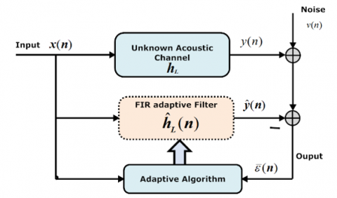
In the context of acoustic echo cancellation (AEC), the identification of unknown hL systems is very important (Figure 1). This system, according to the linear acoustic theory, is a finite impulse response (FIR) model of L taps. The estimated echo signal is described by the following convolution sum:
$\hat{y}(n)=\widehat{\mathbf{h}}_{L}^{T}(n-1) \mathbf{x}_{L}(n)$ (1)
where, $\mathbf{x}_{L}(n)=[x(n), x(n-1), \ldots, x(n-L+1)]^{T}$ is the input signal vector that summarizes the L past samples of the input signal x(n) and $\hat{\mathbf{h}}_{L}(n)=\left[\hat{h}_{0}(n), \hat{h}_{1}(n), \ldots, \hat{h}_{L-1}(n)\right]$ is an estimate of the unknown impulse response hL at time n.
The a priori filtering error $\bar{\varepsilon}(n)$ is given by:
$\bar{\varepsilon}(n)=y(n)-\hat{y}(n)+b(n)$ (2)
where, y(n) and b(n) are the desired signal and the additive noise, respectively.
The general form of the adaptive filter update equation can be written as [25, 26]:
$\hat{\mathbf{h}}_{L}(n)=\widehat{\mathbf{h}}_{L}(n-1)-\mathbf{g}_{L}(n) \bar{\varepsilon}(n)$ (3)
where, the vector gL(n) is called the adaptation gain.
Figure 1. Basic adaptive filter scheme
2.1 The normalized LMS algorithm
The normalized least mean square (NLMS) algorithm is a variant of the LMS algorithm whose adaptation gain is normalized by a quantity proportional to the energy of the input signal xL(n) [25, 27].
$\mathbf{g}_{L}(n)=-\frac{\mu}{\mathbf{x}_{L}{ }^{T}(n) \mathbf{x}_{L}(n)+\delta} \mathbf{x}_{L}(n)$ (4)
where, μ is the adaptation step size bounded between 0 and 2 which is independent of the input signal power, but the choice of the step-size affects directly the convergence speed, the steady state error and the tracking ability of the algorithm. The regularization parameter δ is a small constant used to avoid division by zero, this parameter can be chosen proportional to the power of the input signal: $\delta=\beta \sigma_{x^{2}}$ with β a positive constant [27, 28]. The quantity $\mathbf{x}_{L}^{T}(n) \mathbf{x}_{L}(n)$ can be estimated, with less operations, by the following formula:
$\pi_{\mathrm{x}}(n)=\beta \pi_{\mathrm{x}}(n-1)+(1-\beta) L x^{2}(n)$ (5)
where, β is a forgetting factor.
2.2 The simplified FTF algorithm
The RLS algorithms are based on the minimization, in relation to the vector $\hat{\mathbf{h}}_{L}(n)$, of a deterministic criterion given by the following weighted sum of squared filtering errors [3]:
$j(n)=\sum_{i=1}^{n} \lambda^{n-i}\left[y(i)-\widehat{\mathbf{h}}_{L}^{T}(n) \mathbf{x}_{L}(i)\right]^{2}$ (6)
where, λ denotes an exponential forgetting factor 0<λ<1. These parameter values directly affect the convergence speed, the steady-state error and tracking ability of the algorithm.
The minimization of this last criterion leads to an adaptation gain, called Kalman gain CL(n), defined by:
$\begin{aligned} \mathbf{g}_{L}(n)=C_{L}(n)=& {[C(n), C(n-1), \ldots, C(n-L} \\ &+1)]^{T}=-\boldsymbol{R}_{L}^{-1}(\boldsymbol{n}) \mathbf{x}_{L}(n) \end{aligned}$ (7)
where, RL(n) is the short-term autocorrelation matrix.
The FTF version of FRLS algorithms propagates two forward and backward predictors to update the dual Kalman gain $\widetilde{\boldsymbol{C}}_{L}(n)$ instead of CL(n):
$\boldsymbol{C}_{L}(n)=\gamma(n) \widetilde{\boldsymbol{C}}_{L}(n)$ (8)
where, γ(n) is called the likelihood variable and defined by:
$\gamma(n)=\frac{1}{1-\widetilde{C}_{L}^{T}(n) \mathbf{x}_{L}(n)}$ (9)
Then, the adaptive filter is updated by:
$\hat{\mathbf{h}}_{L}(n)=\hat{\mathbf{h}}_{L}(n-1)-\bar{\varepsilon}(n) \gamma(n) \widetilde{\boldsymbol{C}}_{L}(n)$ (10)
The update equation required for a dual Kalman gain can be defined in a recursive form as follows [13]:
${\left[\begin{array}{c}\widetilde{\boldsymbol{C}}_{L}(n) \\ 0\end{array}\right]=\left[\begin{array}{c}0 \\ \widetilde{\boldsymbol{C}}_{L}(n-1)\end{array}\right]+}$ $\frac{r(n)}{\lambda \beta(n-1)}\left[\begin{array}{c}-\boldsymbol{b}_{L}(n-1) \\ 1\end{array}\right]-\frac{e(n)}{\lambda \alpha(n-1)}\left[\begin{array}{c}1 \\ -\boldsymbol{a}_{L}(n-1)\end{array}\right]$ (11)
where, α(n) and β(n) denote, respectively, forward and backward prediction error variances.
The forward αL(n) and backward bL(n) predictors are obtained from the dual Kalman gain using the following recursive equations:
$\boldsymbol{a}_{L}(n)=\boldsymbol{a}_{L}(n-1)-\gamma(n-1) \widetilde{\boldsymbol{C}}_{L}(n-1) e(n)$ (12.a)
$\boldsymbol{b}_{L}(n)=\boldsymbol{b}_{L}(n-1)-\gamma(n) \widetilde{\boldsymbol{C}}_{L}(n) r(n)$ (12.b)
where, e(n) and r(n) refer respectively to forward and backward prediction errors, which are given by [10,13]:
$e(n)=x(n)-\boldsymbol{a}_{L}^{T}(n-1) \mathbf{x}_{L}(n-1)$ (13.a)
$r(n)=x(n-L)-\boldsymbol{b}_{L}^{T}(n-1) \mathbf{x}_{L}(n)$ (13.b)
In practice, the error accumulation makes the original FTF algorithms numerically unstable due to finite-precision arithmetic operations. In this context, the analysis of the propagation of numerical errors generates stabilization methods without degradation of performance [29, 30].
The theoretical study of error propagation has been carried out in [30] confirming that the source of numerical instability in these algorithms is due to recursive calculations of backward prediction variables. For this reason, backward prediction variables have been completely discarded in SMFTF algorithm in which a dual Kalman gain equation is updated by [13]:
$\left[\begin{array}{c}\widetilde{\boldsymbol{C}}_{L}(n) \\ *\end{array}\right]=\left[\begin{array}{c}0 \\ \widetilde{\boldsymbol{C}}_{L}(n-1)\end{array}\right]-\frac{e(n)}{\lambda \alpha(n-1)+c}\left[\begin{array}{c}1 \\ -\boldsymbol{a}_{L}(n-1)\end{array}\right]$ (14)
where, c is a small regularization constant, * is an unused component and α(n) is a forward prediction error variance given by:
$\alpha(n)=\lambda \alpha(n-1)+\gamma(n-1) e^{2}(n)$ (15)
The forward prediction vector is adjusted by:
$\boldsymbol{a}_{L}(n)=\eta\left[\boldsymbol{a}_{L}(n-1)-e(n) \gamma(n-1) \widetilde{\boldsymbol{C}}_{L}(n-1)\right]$ (16)
where, $\eta$ is a leakage factor close to 1.
3.1 The proposed PU-SMFTF algorithm
In this section, we propose a new FTF-type algorithm with reduced computational complexity by employing the partial update principle. It has been proven that the classical FTF algorithm and their simplified versions decrease only the complexity of the prediction part [31, 32]. However, in the proposed PU-SMFTF algorithm the complexity of the prediction part and the filtering part are reduced using the M-Max method, which selects the most significant coefficients at each iteration. A sub-selected tap-input signal vector has been defined by:
$\widehat{\mathbf{x}}_{L+1}(n)=\mathbf{Q}_{L+1}(n) \mathbf{x}_{L+1}(n)$ (17)
where, the matrix QL+1(n) is defined by:
$\mathbf{Q}_{L+1}(n)=$$\operatorname{diag}\left\{1, q_{0}(n), q_{1}(n), q_{2}(n), \ldots q_{L-1}(n)\right\}=$$\left[\begin{array}{ccccc}1 & 0 & & \cdots & 0 \\ 0 & q_{0}(n) & & \ddots & \vdots \\ \vdots & \ddots & \ddots & & 0 \\ 0 & \cdots & 0 & & q_{L-1}(n)\end{array}\right]_{(L+1) \times(L+1)}$ (18)
The ql(n) terms are given by the M-Max method:
$q_{l}(n)=\left\{\begin{array}{l}1, \text { if }|x(n-l)| \in\{M \text { maxima } \\ \text { components ofthe input } \\ \left.\text { vector }\left|\mathbf{x}_{L}(n)\right|\right\} \\ 0, \text { else }\end{array}\right.$ (19)
For index l=0, 1, …, L-1.
The method for selecting ql(n) coefficients is part of a technique used in fast sorting algorithms [33, 34]. The complexity of this type of algorithm can be seen in terms of number of additions only, which in fact does not affect the number of multiplications of the complexity of the proposed algorithm. We note that after sorting and selecting, the vector $\hat{\mathbf{x}}_{L+1}(n)$ contains only M non-zero components.
To compute the new dual Kalman gain update equation, we use the following inversion lemma of a partitioned matrix [35]:
$\boldsymbol{R}_{L+1}^{-1}(n)=\left[\begin{array}{cc}0 & 0 \\ 0 & \boldsymbol{R}_{L}^{-1}(n-1)\end{array}\right]+\left[\begin{array}{c}1 \\ -\boldsymbol{a}_{L}(n)\end{array}\right]\left[\begin{array}{ll}1 & \left.-\boldsymbol{a}_{L}^{\boldsymbol{T}}(n)\right] \frac{1}{\alpha(n)}\end{array}\right.$ (20.a)
$\boldsymbol{R}_{L+1}^{-\boldsymbol{1}}(n)=\left[\begin{array}{cc}\boldsymbol{R}_{L}^{-1}(n-1) & 0 \\ 0 & \mathbf{0}\end{array}\right]+\left[\begin{array}{c}-\boldsymbol{b}_{L}(n) \\ 1\end{array}\right]\left[\begin{array}{ll}-\boldsymbol{b}_{L}(n) & 1\end{array}\right] \frac{1}{\beta(n)}$ (20.b)
By taking Eqns. (20) at time n-1 and right multiplying by $\frac{1}{\lambda_{P U}} \hat{\mathbf{x}}_{L+1}(n)$, we obtain the new dual Kalman gain update equations of order L+1:
$\widetilde{\boldsymbol{C}}_{L+1}(n)=\left[\begin{array}{c}0 \\ \widetilde{\boldsymbol{C}}_{L}(n-1)\end{array}\right]-$$\frac{e_{P U}(n)}{\lambda_{P U} \alpha_{P U}(n-1)+c}\left[-\boldsymbol{a}_{L}(n-1) \mathbf{Q}_{L}(n)\right]$ (21.a)
$\widetilde{\boldsymbol{C}}_{L+1}(n)=\left[\begin{array}{c}\widetilde{\boldsymbol{C}}_{L}(n) \\ 0\end{array}\right]+$$\frac{r(n)}{\lambda_{P U} \beta(n-1)}\left[\begin{array}{c}-\boldsymbol{b}_{L}(n-1) \mathbf{Q}_{L}(n) \\ 1\end{array}\right]$ (21.b)
By merging the two equations Eq. (21.a) and Eq. (21.b) and discarding the backward prediction variables, we get the update equation of the dual Kalman gain for the proposed algorithm:
$\left[\begin{array}{c}\widetilde{\boldsymbol{C}}_{L}(n) \\ *\end{array}\right]=\left[\begin{array}{c}0 \\ \widetilde{\boldsymbol{C}}_{L}(n-1)\end{array}\right]-$$\frac{e_{P U}(n)}{\lambda_{P U} \alpha_{P U}(n-1)+c}\left[\begin{array}{c}1 \\ -\boldsymbol{a}_{L}(n-1) \mathbf{Q}_{L}(n)\end{array}\right]$ (22)
with:
$e_{P U}(n)=x(n)-\boldsymbol{a}_{L}^{T}(n-1) \hat{\mathbf{x}}_{L}(n-1)$ (22.a)
$\alpha_{P U}(n)=\lambda_{P U} \alpha_{P U}(n-1)+\gamma_{P U}(n-1) e_{P U}^{2}(n)$ (22.b)
$\boldsymbol{a}_{L}(n)=\eta\left[\boldsymbol{a}_{L}(n-1) \mathbf{Q}_{L}(n)-e_{P U}(n) \gamma_{P U}(n-1) \widetilde{\boldsymbol{C}}_{L}(n-1) \mathbf{Q}_{L}(n)\right]$ (22.c)
And
$\gamma_{P U}(n)=\frac{1}{1-\widetilde{\boldsymbol{C}}_{L}^{T}(n) \widehat{\mathbf{x}}_{L}(n)}$ (22.d)
The computational complexity of this prediction part of the proposed PU-SMFTF algorithm becomes 5M+7 multiplications per iteration.
The new update equation for $\hat{\mathbf{h}}_{L}(n)$ becomes:
$\widehat{\mathbf{h}}_{L}(n)=\widehat{\mathbf{h}}_{L}(n-1)-\bar{\varepsilon}(n) \gamma_{P U}(n) \mathbf{Q}_{L}(n) \widetilde{\boldsymbol{C}}_{L}(n)$ (23)
This last equation and the filtering error formula need L+M+1 multiplications. Thus, the total arithmetic operations of the proposed algorithm are L+6M+8 multiplications. This complexity becomes lower than that of the NLMS algorithm for $M \leq \frac{L-2}{6}$. The proposed PU-SMFTF is summarized in Table 1.
Table 1. The proposed PU-SMFTF algorithm
|
Initialization |
|
$\boldsymbol{a}_{L}(0)=\mathbf{0}, \widetilde{\boldsymbol{C}}_{L}(0)=\mathbf{0}, \hat{\mathbf{h}}_{L}(0)=\mathbf{0}$ $\gamma_{P U}(0)=1, \alpha_{P U}(0)=E_{0} \lambda_{p u}^{L}$ with $E_{0}$ initial value. |
|
Adaptation for n=1;2;.. |
|
Choice of the selection matrix $\mathbf{Q}_{L}(n)=\operatorname{diag}\left\{q_{0}(n), q_{1}(n), q_{2}(n), \ldots q_{L-1}(n)\right\}$ $q_{l}(n)= \begin{cases}1, & \text { if }|x(n-l)| \in\left\{M \text { maxima components ofthe input vector }\left|\mathbf{x}_{L}(n)\right|\right\} \\ 0, & \text { else }\end{cases}$ For index $l=0,1, \ldots, L-1$. Prediction part - Forward prediction error $\widehat{\mathbf{x}}_{L}(n-1)=\mathbf{Q}_{L}(n) \mathbf{x}_{L}(n-1), \widehat{\mathbf{x}}_{L}(n)=\mathbf{Q}_{L}(n) \mathbf{x}_{L}(n)$ $e_{P U}(n)=x(n)-\boldsymbol{a}_{L}^{T}(n-1) \widehat{\mathbf{x}}_{L}(n-1)$ $\alpha_{P U}(n)=\lambda_{P U} \alpha_{P U}(n-1)+\gamma_{P U}(n-1) e_{P U}^{2}(n)$ Adaptation gain vector $\left[\begin{array}{c}\widetilde{\boldsymbol{C}}_{L}(n) \\ *\end{array}\right]=\left[\begin{array}{c}0 \\ \widetilde{\boldsymbol{C}}_{L}(n-1)\end{array}\right]-\frac{e_{P U}(n)}{\lambda_{P U} \alpha_{P U}(n-1)+c}\left[\begin{array}{c}1 \\ -\boldsymbol{a}_{L}(n-1) \mathbf{Q}_{L}(n)\end{array}\right]$ Forward predictor $\boldsymbol{a}_{L}(n)=\eta\left\lceil\boldsymbol{a}_{L}(n-1) \mathbf{Q}_{L}(n)-e_{P U}(n) \gamma_{P U}(n-1) \widetilde{\boldsymbol{C}}_{L}(n-1) \mathbf{Q}_{L}(n)\right\rceil$ Likelihood variable $\gamma_{P U}(n)=\frac{1}{1-\widetilde{\boldsymbol{C}}_{L}^{T}(n) \widehat{\mathbf{x}}_{L}(n)}$ Filtering part $\bar{\varepsilon}(n)=y(n)-\widehat{\mathbf{h}}_{L}^{1}(n-1) \mathbf{x}_{L}(n)$ $\widehat{\mathbf{h}}_{L}(n)=\widehat{\mathbf{h}}_{L}(n-1)-\bar{\varepsilon}(n) \gamma_{P U}(n) \mathbf{Q}_{L}(n) \widetilde{\boldsymbol{C}}_{L}(n)$ |
3.2 The proposed RPU-SMFTF algorithm
The idea of a reduced size predictor was successfully used in the SMFTF algorithm [13]. Here, we propose to further reduce the computation complexity by incorporating the technique of partial update in the PU-SMFTF algorithm with a forward predictor for a smaller size P compared to the size L of the adaptive filter. The extension of this idea to the PU-SMFTF algorithm requires the following steps:
Step 1:
We limit the size of the forward predictor vector to a reduced size P≤L, with $\boldsymbol{a}_{\boldsymbol{P}}(n)=[a(n), a(n-1), \ldots, a(n-P+1)]$, so the forward prediction error is written as:
$e_{p}(n)=x(n)-\boldsymbol{a}_{P}^{\boldsymbol{T}}(n-1) \mathbf{x}_{P}(n-1)$ (24)
Step 2:
We will use an extrapolation method to calculate the dual Kalman gain and the likelihood variable of order L. The forward predictor and dual Kalman gain are given respectively by:
$a_{L}(n-1)=\left[\begin{array}{c}a_{P}(n-1) \\ 0_{L-P}\end{array}\right]$ (25)
${\left[\begin{array}{c}\widetilde{\boldsymbol{C}}_{L}(n) \\ c_{L+1}(n)\end{array}\right]=\left[\begin{array}{c}0 \\ \widetilde{\boldsymbol{C}}_{L}(n-1)\end{array}\right]-}$$\frac{e_{P}(n)}{\lambda_{R P U}\quad \alpha_{P}(n-1)+c}\left[\begin{array}{c}1 \\ -\boldsymbol{a}_{L}(n-1)\end{array}\right]$ (26)
where, 0L-P is a zero vector of order (L-P). We note cL+1(n) the unused component and cP+1(n) the (P+1)th component of $\widetilde{\boldsymbol{C}}_{L}(n)$.
The new update information of dual Kalman gain is located in the (P+1) first components and the last values are offset versions of the (P+1)th component of $\widetilde{\boldsymbol{C}}_{L}(n)$ [12]. In order to reduce the computational complexity much more, for this algorithm, we considered two likelihood variables [36]. The first one, γP(n), is used to update the forward prediction variables:
$\gamma_{P}(n)=\frac{\gamma_{P}(n-1)}{1+\gamma_{P}(n-1) \vartheta_{P}(n)}$ (27)
where,
$\vartheta_{P}(n)=\frac{e_{P}^{2}(n)}{\lambda_{R P U} \quad\alpha_{P}(n-1)+c}+c_{P+1}(n) x(n-P)$ (28)
The second likelihood variable γL(n) is used to update the adaptive filter $\hat{\mathbf{h}}_{L}(n)$:
$\gamma_{L}(n)=\frac{\gamma_{L}(n-1)}{1+\gamma_{L}(n-1) \vartheta_{L}(n)}$ (29)
$\vartheta_{L}(n)=\frac{e_{P}^{2}(n)}{\lambda_{R P U} \quad\alpha_{P}(n-1)+c}+c_{L+1}(n) x(n-L)$ (30)
Step 3:
We will choose the M coefficients of the dual Kalman vector $\widetilde{\boldsymbol{C}}_{L}(n)$ which are the most significant in amplitudes using the diagonal selection matrix QL(n), and then we update the adaptive filter weights by:
$\hat{\mathbf{h}}_{L}(n)=\hat{\mathbf{h}}_{L}(n-1)-\bar{\varepsilon}(n) \gamma_{L}(n) \mathbf{Q}_{L}(n) \widetilde{\boldsymbol{C}}_{L}(n)$ (31)
A summary of the proposed algorithm is given in Table 2.
Table 2. The proposed RPU-SMFTF algorithm
|
Initialization |
|
$\boldsymbol{a}_{L}(0)=\mathbf{0}, \widetilde{\boldsymbol{C}}_{L}(0)=\mathbf{0}, \hat{\mathbf{h}}_{L}(0)=\mathbf{0}$, $\gamma_{L}(0)=\gamma_{P}(0)=1, \alpha_{p}(0)=E_{0} \lambda_{R P U}^{P}$ with $E_{0}$ initial value. |
|
Adaptation for n=1;2;.. |
|
Choice of the selection matrix $\mathbf{Q}_{L}(n)=\operatorname{diag}\left\{q_{0}(n), q_{1}(n), q_{2}(n), \ldots q_{L-1}(n)\right\}$ $q_{l}(n)=$$\left\{\begin{array}{l}1, \text { if }|x(n-l)| \in\left\{M \text { maxima components ofthe input vector }\left|\mathbf{x}_{L}(n)\right|\right\} \\ 0, \text { else }\end{array}\right.$ For index $l=0,1, \ldots, L-1$. Prediction part - Forward prediction error $e_{P}(n)=x(n)-\boldsymbol{a}_{\boldsymbol{P}}^{\boldsymbol{T}}(\boldsymbol{n}-\mathbf{1}) \mathbf{x}_{\boldsymbol{P}}(\boldsymbol{n}-\mathbf{1})$ $\alpha_{P}(n)=\lambda_{R P U} \alpha_{P}(n-1)+\gamma_{P}(n-1) e_{P}^{2}(n)$ Adaptation gain vector $\boldsymbol{a}_{L}(n-1)=\left[\begin{array}{c}\boldsymbol{a}_{\boldsymbol{P}}(n-1) \\ \mathbf{0}_{N-P}\end{array}\right]$ ${\left[\begin{array}{c}\widetilde{\boldsymbol{C}}_{L}(n) \\ c_{L+1}(n)\end{array}\right]=\left[\begin{array}{c}0 \\ \widetilde{\boldsymbol{C}}_{L}(n-1)\end{array}\right]-}$$\frac{e_{P}(n)}{\lambda_{R P U} \alpha_{P}(n-1)+c}\left[\begin{array}{c}1 \\ -\boldsymbol{a}_{L}(n-1)\end{array}\right]$ Forward predictor $\boldsymbol{a}_{\boldsymbol{P}}(\boldsymbol{n})=\eta\left[\boldsymbol{a}_{\boldsymbol{P}}(\boldsymbol{n}-\mathbf{1})-e_{P}(n) \gamma_{P}(n-1) \widetilde{\boldsymbol{C}}_{\boldsymbol{P}}(\boldsymbol{n}-\mathbf{1})\right]$ Likelihood variables $\begin{aligned} \vartheta_{P}(n) &=\frac{e_{P}^{2}(n)}{\lambda_{R P U} \alpha_{P}(n-1)+c}+c_{P+1}(n) x(n-P), \\ \gamma_{P}(n) &=\frac{\gamma_{P}(n-1)}{1+\gamma_{P}(n-1) \vartheta_{P}(n)} \\ \vartheta_{L}(n) &=\frac{e_{P}^{2}(n)}{\lambda_{R P U} \alpha_{P}(n-1)+c}+c_{L+1}(n) x(n-L), \\ \gamma_{L}(n)=& \frac{\gamma_{L}(n-1)}{1+\gamma_{L}(n-1) \vartheta_{L}(n)} \end{aligned}$ Filtering part $\bar{\varepsilon}(n)=y(n)-\hat{\mathbf{h}}_{L}^{T}(n-1) \mathbf{x}_{L}(n)$ $\widehat{\mathbf{h}}_{L}(n)=\hat{\mathbf{h}}_{L}(n-1)-\bar{\varepsilon}(n) \gamma_{L}(n) \mathbf{Q}_{L}(n) \widetilde{\boldsymbol{C}}_{L}(n)$ |
In this section, we compare the performances of PU-SMFTF and RPU-SMFTF algorithms with the classical SMFTF, NLMS and PU-NLMS algorithms [31]. Series of experiments are carried out with stationary and non-stationary signals and systems to validate the superiority of the proposed algorithms in terms of complexity reduction and the ability of tracking changes in input signals and impulse responses. The performances are evaluated using an estimate of the change over time of the mean square error (MSE) defined by:
$M S E_{d B}(n)=10 \log _{10}\left(\left\langle\bar{\varepsilon}(n)^{2}\right\rangle\right)$ (32)
where, $\langle.\rangle$ is a short-time average over a small number of samples.
4.1 Simulation parameters
4.1.1 Description of signals and systems
In order to show the convergence speed and the behavior of the proposed algorithms in case of acoustic channel variation, a common stationary noise called USASI (USA Standards Institute) is used as input signal. This latter has a normal probability distribution, a variance equals $\sigma_{x}^{2}=0.32$ and a dynamic range of the frequency spectrum of about 29 dB.
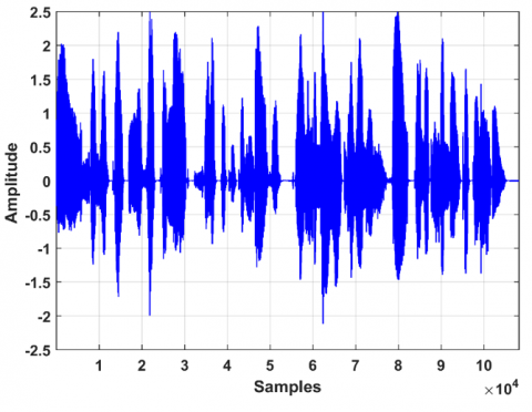
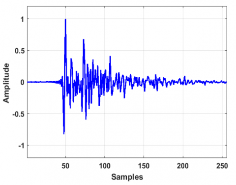
In a real time, acoustic echo situation, we tested the algorithms with a non-stationary real speech signal (Figure 2) of spectral dynamics of about 40 dB. The power of this speech signal is $\sigma_{x}^{2}=0.17$. Desired signals are obtained by convolution of a real acoustic impulse response with the input signals, and then truncated to 256 points (Figure 3). An additive white Gaussian noise is added to echo signal with a given signal-to-noise ratio, to show the performances of the proposed algorithms in case of noisy environments. All these signals are sampled with a frequency of 16 kHz.
4.1.2 Choice of algorithm parameters
The key parameters must be set properly for a fair comparison of the tested algorithms. For the NLMS and PU-NLMS algorithms, the value of the adaptation step that gives us the best convergence speed is set to μ=1 with no output noise and slightly lower than one for a noisy desired signal [27, 37]. The regularization constants, for all tested algorithms, are fixed to a value proportional to the average energy of the input signal: $\delta=c=1(\beta \approx 3$ for USASI signal and $\beta \approx 6$ for Speech $)$.
Figure 2. Speech signal
Figure 3. Real acoustic impulse response measured in car cabin (size of 256 samples)
The initial value of the forward prediction error variance $E_{0}$ must be chosen to ensure the initial start of the algorithm. This constant is set to one for a normalized input signal x(n). The typical value of forgetting factor λ that provides good performances of the original SMFTF was set to λ=0.9989. In addition, forgetting factors of the proposed algorithms must be well chosen to ensure good convergence speed and tracking ability. We set λPU=0.997 for the first proposed algorithm and λRPU=0.85 for the second proposed algorithm in the coming experiments. For proper working of the forward predictor, in particular in speech silence intervals, the leakage factor is set to η=0.985 for SMFTF and PU-SMFTF, and to η=0.992 for the proposed RPU-SMFTF.
4.2 Case of a stationary input signal
In this part of simulation, we used the USASI noise as input and $L=256$ for the size of the unknown system (Figure 3 ). The number $M$ of coefficients to be selected has been chosen so that a best convergence speed and a lower arithmetic operation are ensured for the proposed algorithm. To attain this solution, we put $M=\frac{L}{2}$.
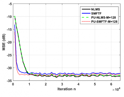
Figures 4 and 5 illustrate the comparison of the proposed PU-SMFTF algorithm with the conventional NLMS, PU-NLMS and SMFTF algorithms with two signal-to-noise ratio (SNR) values of 50 dB and 30 dB, respectively. These results show a superiority of convergence speed of the proposed algorithm compared to other tested algorithms. The proposed PU-SMFTF algorithm provides similar performance in terms of final MSE compared with the other classical algorithms, but with a lower complexity.
Figure 4. The MSE evolution of PU-SMFTF, SMFTF, NLMS and PU-NLMS algorithms for stationary USASI noise, $L=256$ and Output noise with SNR=50 dB
Figure 5. Learning curves of PU-SMFTF, SMFTF, NLMS and PU-NLMS algorithms for stationary USASI noise, $L=256$ and SNR=30 dB
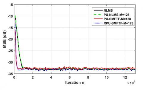
Figure 6. MSE evolution of RPU-SMFTF, NLMS and PU-NLMS algorithm for stationary USASI noise, RPU-SMFTF ( $\lambda_{R P U}$ =0.85), SNR=30
Figure 6 shows the MSE of the proposed RPU-SMFTF algorithm in comparison with NLMS and PU-NLMS algorithms. The order of the reduced predictor is P=8 and the number of coefficients to be adapted by iteration in this case is fixed at $M=\frac{L}{2}$. From this figure, it can be seen that the proposed algorithms give much better convergence speed than NLMS and PU-NLMS algorithms.
4.3 Case of non-stationary system
In this experiment, we compare the performances in terms of convergence rate and tracking ability of the proposed algorithms with the classical NLMS and SMFTF algorithms. For this purpose, a continuous variation of the unknown system is made by introducing an artificial linear gain in the echo path. This is generated by multiplying the echo signal $y(n)$ by a triangular gain function of amplitude between 1 and 2.5 (Figure 7). The gain variation starts at iteration 50000 and ends at iteration 80000.
Figure 8 shows that the proposed algorithms converge faster and track better the variations of the impulse response than the SMFTF algorithm, with the same steady-state MSE. It is worth noting that the proposed PU-type algorithm achieves gains of approximately 8 dB compared to SMFTF and about 12 dB compared to NLMS during echo path variation period.
Figure 7. Artificial gain variation for the experiment of testing the tracking performance
Figure 8. Comparison of tracking capability of various adaptive algorithms with an stationary input signal (USASI), Output with SNR=70dB, $L=256$ and $P=8$
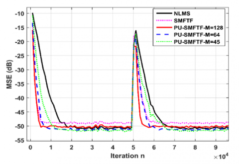
4.4 The effect of the size M
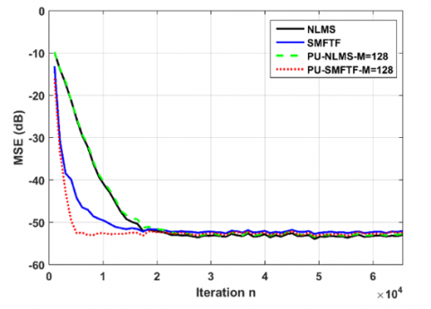
Figure 9 depicts the MSE learning curves for $M=128$, $M=64$ and $M=45$ coefficients in the partial update based algorithms. In this experiment, we create a sudden change in the echo path by multiplying the desired signal by $1.5$ at the iteration $n=50000$. These results show slight degradations on the MSE when $M$ decreases to 128,64 and 45 coefficients compared to the SMFTF algorithm with 256 coefficients. We also note that these performances remain better than those of the NLMS algorithm with $L=256$.
Figure 9. Effects of the size M on the PU-SMFTF algorithm for $L=256$ and Output with SNR $=50 \mathrm{~dB}$
4.5 Effects of the P-size forward predictor
Figure 10 shows the effect of decreasing predictor order $P$ on the behaviour of RPU-SMFTF algorithm for a stationary input signal and a filter size $L=256$. This experiment shows that the proposed RPU-SMFTF has the best performance in terms of convergence, re-convergence rate than the other classical-type tested algorithms, for the three different order size $P$.
Figure 10. Effects of the size P value on the RPU-SMFTF algorithm for $L=256$ and $M=\frac{L}{2}$
4.6 Case of non-stationary input
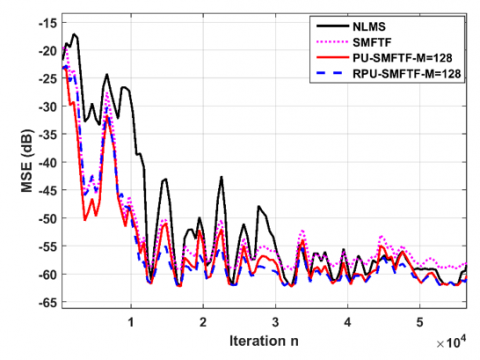
Figure 11. Comparison with speech signal, PU-SMFTF $\left(\lambda_{P U}=0.9985\right)$, SMFTF $(\lambda=0.9989)$, RPU-SMFTF $\left(\lambda_{R P U}=0.985\right), \eta=0.98, c=0.1$ and $\mathrm{SNR}=50 \mathrm{~dB}$
Figure 11 depicts the MSE performance curves of the NLMS, SMFTF, PU-SMFTF and RPU-SMFTF algorithms with a speech as input under impulse response of length L = 256. The forward predictor order is fixed to P=15. The leakage factor for all algorithms is taken $\eta=0.98$. Parameters of the NLMS algorithm remain unchanged from the previous simulations. This experiment demonstrates that the NLMS algorithm has difficulties to identify the unknown system. These difficulties are caused by the high degree of correlation of the speech signal. In addition, it can be seen from Figure 11 that the PU-SMFTF and RPU-SMFTF outperform the other tested algorithms in the transient and the steady-state phases, with lower computational cost.
4.7 Computational complexity evaluation
In this subsection, we have evaluated the computational complexities, based on the number of arithmetic multiplications only, of the proposed PU-SMFTF and RPU-SMFTF algorithms compared to the classical SMFTF and NLMS algorithms.
Table 3 summarizes the complexities for the considered algorithms. Figure 12 presents numerical example for different values of M and with fixed L=256 and P=8. It has been found that, the computational complexities of the proposed algorithms are lower than the complexity of the NLMS algorithm with performances better than both NLMS and SMFTF algorithms.
Table 3. Comparison of computational complexities
|
Complexity in multiplications per iteration |
|||
|
Algorithms |
Prediction part |
Filtering part |
Full complexity |
|
NLMS |
0 |
2L+6 |
2L+6 |
|
SMFTF [13] |
5L+7 |
2L+1 |
7L+8 |
|
PU-SMFTF |
5M+7 |
L+M+1 |
L+6M+8 |
|
RPU-SMFTF |
4P+16 |
L+M+1 |
L+M++4P+17 |
Figure 12. Numerical comparison of the computational complexities
In this paper, we have proposed two new adaptive filtering algorithms derived from the SMFTF algorithm by incorporating the partial update technique in both filtering and prediction parts, in order to get a reduced complexity and a higher convergence speed. We have compared the performances of the proposed algorithms with those of the SMFTF and NLMS algorithms under different scenarios, such as variable acoustic channel and noisy environments. Based on the results, it can be concluded that the proposed algorithms present better performances in terms of convergence and re-convergence speed than the NLMS and the SMFTF algorithms.
In addition, these interesting performances are obtained with a complexity much lower than other tested algorithms for small values of $M$. The computational complexity has been reduced from $7 L+8$ to $L+6 M+8$ (with $M<<L$ ) for the proposed PU-SMFTF algorithm and becomes $L+M+$ $4 P+17$ for the RPU-SMFTF algorithm of $P$-size forward predictor (with $P \ll M \ll L$ ). Also, it has been shown that the proposed algorithms have better capability to track the variations of the unknown system.
|
AEC |
Acoustic Echo Cancellation |
|
FIR |
Finite Impulse Response |
|
FK |
Fast Kalman |
|
FAEST |
Fast a posteriori Error Sequential Technique |
|
FNLMS |
Fast NLMS |
|
FNFTF |
Fast Newton Transversal Filter |
|
FTF |
Fast Transversal Filter |
|
MSE |
Mean Square Error |
|
NLMS |
Normalized Least Mean Square |
|
PU |
Partial Update |
|
RLS RLS |
Recursive Least Square |
|
RPU |
Reduced Partiel Update |
|
SMFTF |
Simplified FTF |
|
SNR |
Signal to Noise Ratio |
|
USASI |
USA Standards Institute (ANSI) |
|
Greek symbols |
|
|
$\alpha(n)$ |
Forward Error Variance |
|
$\beta(\mathrm{n})$ |
Backward Error Variance |
|
$\gamma(\mathrm{n})$ |
Likelihood Variable |
|
µ |
Step-size |
|
ƛ |
Forgetting Factor |
|
Subscripts |
|
|
P |
Size of the reduced Predictor |
|
L |
Size of the Adaptive Filter |
[1] Diniz, P.S.R. (2020). Fundamentals of adaptive filtering. Adaptive Filtering, 9-60. https://doi.org/10.1007/978-3-030-29057-3_2
[2] Comon, P., Jutten, C. (2010). Handbook of Blind Source Separation: Independent Component Analysis and Applications. Academic Press.
[3] Haykin, S.S. (2014). Adaptive Filter Theory. 5th ed. Pearson Education India.
[4] Hamidia, M., Amrouche, A. (2016). Improved variable step-size NLMS adaptive filtering algorithm for acoustic echo cancellation. Digital Signal Processing, 49: 44-55. https://doi.org/10.1016/J.DSP.2015.10.015
[5] Yu, W., Kleijn, W.B. (2021). Room acoustical parameter estimation from room impulse responses using deep neural networks. IEEE/ACM Transactions on Audio, Speech, and Language Processing, 29: 436–447. https://doi.org/10.1109/taslp.2020.3043115
[6] Benziane, M., Bouamar, M., Makdir, M. (2020). Simple and efficient double-talk-detector for acoustic echo cancellation. Traitement du Signal, 37(4): 585-592. https://doi.org/10.18280/ts.370406
[7] Uncini, A. (2015). Fundamentals of Adaptive Signal Processing. Springer.
[8] Carayannis, G., Manolakis, D., Kalouptsidis, N. (1983). A fast sequential algorithm for least-squares filtering and prediction. IEEE Transactions on Acoustics, Speech, and Signal Processing, 31(6): 1394-1402. https://doi.org/10.1109/TASSP.1983.1164224
[9] González, A., Ferrer, M., de Diego, M., Piñero, G., López, J.J. (2005). Practical implementation of multichannel adaptive filters based on FTF and AP algorithms for active control. International Journal of Adaptive Control and Signal Processing, 19(2-3): 89-105. https://doi.org/10.1002/ACS.845
[10] Cioffi, J., Kailath, T. (1984). Fast, recursive-least-squares transversal filters for adaptive filtering. IEEE Transactions on Acoustics, Speech, and Signal Processing, 32(2): 304-337. https://doi.org/10.1109/TASSP.1984.1164334
[11] Mavridis, P.P., Moustakides, G.V. (1996). Simplified newton-type adaptive estimation algorithms. IEEE Transactions on Signal Processing, 44: 1932–1940. https://doi.org/10.1109/78.533714
[12] Petillon, T., Gilloire, A., Theodoridis, S. (1994). The fast Newton transversal filter: An efficient scheme for acoustic echo cancellation in mobile radio. IEEE Transactions on Signal Processing, 42(3): 509-518. https://doi.org/10.1109/78.277843
[13] Benallal, A., Benkrid, A. (2007). A simplified FTF-type algorithm for adaptive filtering. Signal Processing, 87(5): 904-917. https://doi.org/10.1016/J.SIGPRO.2006.08.013
[14] Arezki, M., Benallal, A., Guessoum, A., Berkani, D. (2008). Improvement of the simplified FTF-Type algorithm. In SIGMAP, 156-161. https://doi.org/10.5220/0001940001560161
[15] Benallal, A., Arezki, M. (2014). A fast convergence normalized least‐mean‐square type algorithm for adaptive filtering. International Journal of Adaptive Control and Signal Processing, 28(10): 1073-1080. https://doi.org/10.1002/acs.2423
[16] Mayyas, K. (2013). A variable step-size selective partial update LMS algorithm. Digital Signal Processing, 23(1): 75-85. https://doi.org/10.1016/J.DSP.2012.09.004
[17] Zhou, Y., Chan, S.C., Ho, K.L. (2010). New sequential partial-update least mean M-estimate algorithms for robust adaptive system identification in impulsive noise. IEEE Transactions on Industrial Electronics, 58(9): 4455-4470. https://doi.org/10.1109/TIE.2010.2098359
[18] Khong, A.W., Naylor, P.A. (2006). Stereophonic acoustic echo cancellation employing selective-tap adaptive algorithms. IEEE Transactions on Audio, Speech, and Language Processing, 14(3): 785-796. https://doi.org/10.1109/TSA.2005.858065
[19] Le, D. C., Li, D., Zhang, J. (2019). M-max partial update leaky bilinear filter-error least mean square algorithm for nonlinear active noise control. Applied Acoustics, 156: 158-165. https://doi.org/10.1016/J.APACOUST.2019.07.006
[20] Mayyas, K., Afeef, L. (2020). A variable step-size partial-update normalized least mean square algorithm for second-order adaptive volterra filters. Circuits, Systems, and Signal Processing, 39(12): 6073-6097. https://doi.org/10.1007/S00034-020-01446-2
[21] Bismor, D. (2016). Simulations of partial update LMS algorithms in application to active noise control. Procedia Computer Science, 80: 1180-1190. https://doi.org/10.1016/J.PROCS.2016.05.451
[22] Wen, H.X., Yang, S.Q., Hong, Y.Q., Luo, H. (2019). A partial update adaptive algorithm for sparse system identification. IEEE/ACM Transactions on Audio, Speech, and Language Processing, 28: 240-255. https://doi.org/10.1109/TASLP.2019.2949928
[23] Kalouptsidis, N., Mileounis, G., Babadi, B., Tarokh, V. (2011). Adaptive algorithms for sparse system identification. Signal Processing, 91(8): 1910-1919. https://doi.org/10.1016/j.sigpro.2011.02.013
[24] Hassani, I., Kedjar, A., Ramdane, M.A., Arezki, M., Benallal, A. (2018). Fast sparse adaptive filtering algorithms for acoustic echo cancellation. In 2018 International Conference on Communications and Electrical Engineering (ICCEE), pp. 1-5. https://doi.org/10.1109/CCEE.2018.8634473
[25] Yang, B. (2020). An adaptive filtering algorithm for non-gaussian signals in alpha-stable distribution. Traitement du Signal, 37(1): 69-75. https://doi.org/10.18280/ts.370109
[26] Hassani, I., Arezki, M., Benallal, A. (2020). A novel set membership fast NLMS algorithm for acoustic echo cancellation. Applied Acoustics, 163: 107210. https://doi.org/10.1016/j.apacoust.2020.107210
[27] Paleologu, C., Ciochină, S., Benesty, J., Grant, S.L. (2015). An overview on optimized NLMS algorithms for acoustic echo cancellation. EURASIP Journal on Advances in Signal Processing, 2015(1): 1-19. https://doi.org/10.1186/S13634-015-0283-1
[28] Slock, D.T. (1993). On the convergence behavior of the LMS and the normalized LMS algorithms. IEEE Transactions on Signal Processing, 41(9): 2811-2825. https://doi.org/10.1109/78.236504
[29] Ferreira, E.F., Rêgo, P.H., Neto, J.V. (2017). Numerical stability improvements of state-value function approximations based on RLS learning for online HDP-DLQR control system design. Engineering Applications of Artificial Intelligence, 63: 1-19. https://doi.org/10.1016/J.ENGAPPAI.2017.04.017
[30] Bunch, J.R., Le Borne, R.C., Proudler, I.K. (2003). Applying numerical linear algebra techniques to analyzing algorithms in signal processing. Linear Algebra and Its Applications, 361: 133-146. https://doi.org/10.1016/S0024-3795(02)00318-X
[31] Aboulnasr T, Mayyas K. (1999). Complexity reduction of the NLMS algorithm via selective coefficient update. IEEE Transactions on Signal Processing, 47(5): 1421-1424. https://doi.org/10.1109/78.757235
[32] Mayyas, K. (2013). Performance analysis of the selective coefficient update NLMS algorithm in an undermodeling situation. Digital Signal Processing, 23(6): 1967-1973. https://doi.org/10.1016/J.DSP.2013.07.006
[33] Pitas, I. (1989). Fast algorithms for running ordering and max/min calculation. IEEE Transactions on Circuits and Systems, 36(6): 795-804. https://doi.org/10.1109/31.90400
[34] Brookes, M. (2000). Algorithms for max and min filters with improved worst-case performance. IEEE Transactions on Circuits and Systems II: Analog and Digital Signal Processing, 47(9): 930-935. https://doi.org/10.1109/82.868461
[35] Swami, A. (1996). Fast transversal versions of the RIV algorithm. International Journal of Adaptive Control and Signal Processing, 10(2-3): 267-281. https://doi.org/10.1002/(SICI)1099-1115(199603)10:2/3<267::AID-ACS350>3.0.CO;2-4
[36] Arezki, M., Namane, A., Benallal, A., Meyrueis, P., Berkani, D. (2012). Fast adaptive filtering algorithm for acoustic noise cancellation. In Proc. the World Congress on Engineering, 2.
[37] Benesty, J., Paleologu, C., Ciochina, S. (2010). On regularization in adaptive filtering. IEEE Transactions on Audio, Speech, and language Processing, 19(6): 1734-1742. https://doi.org/10.1109/TASL.2010.2097251