Naser Sadeghi Gharagoz* | Ali Can Karaca
© 2026 The authors. This article is published by IIETA and is licensed under the CC BY 4.0 license (http://creativecommons.org/licenses/by/4.0/).
OPEN ACCESS
The vast amount of data generated by multispectral (MS) satellites makes image compression critical for remote sensing applications, as storing, processing, and downlinking these volumes to ground stations poses significant challenges. Temporal correlations in multitemporal images captured on different dates of the same scene can improve compression efficiency. This study builds on MultiTempGAN, a generative adversarial network (GAN) that predicts target MS images from reference MS images and improves model efficiency by applying 6-bit post-training non-uniform quantization (NUQ) to the generator without retraining, via piecewise linear quantization (PLQ). Experiments on Sentinel-2 MS image pairs reveal that 6-bit PLQ improves Laplacian mean square error (LMSE), signal-to-noise ratio (SNR), and bits-per-pixel (bpp) metrics compared to those of Q-MultiTempGAN, the uniformly quantized version of MultiTempGAN. Relative to full-precision MultiTempGAN, it incurs only a 0.46% decrease in SNR and a 33.33% increase in LMSE, yet achieves an 81.18% reduction in bpp. These results demonstrate that 6-bit PLQ yields a significantly smaller model with minimal loss in reconstruction accuracy, supporting more practical deployment of temporal-prediction-based MS compression.
multispectral image compression, generative adversarial networks, model quantization, non-uniform quantization, model compression, multitemporal images
The proliferation of Earth observation satellites has led to an expanding archive of MS imagery, providing essential data for a variety of remote sensing applications. Systems such as Sentinel-2 conduct continuous surveillance of the Earth's surface, acquiring high-resolution images of identical locations over successive periods. This large dataset is of critical importance for environmental studies, precision agriculture, and disaster response. However, with predictions indicating an exponential increase in data volume over the coming 30 years, the need for efficient storage and transmission solutions is becoming increasingly critical. This makes compression an unavoidable necessity.
Traditional image compression methods such as JPEG2000 (JP2K) have been widely adopted for MS image compression. At its core, JP2K relies on the discrete wavelet transform (DWT) to address spatial redundancies, while various enhanced JP2K configurations have been developed to tackle specific compression challenges [1]. The integration of DWT with JP2K (JP2K+DWT) improves compression performance by emphasizing fine details and reducing spatial redundancy [2], while principal component analysis (PCA) can be incorporated to reduce spectral dimensionality with minimal information loss [3].
Zhang et al. [4] propose PMLabPQR, a novel polynomial-regression-based Interim Connection Space (ICS) that enhances spectral reconstruction accuracy while reducing additional data overhead. By replacing the traditional R matrix with a learned polynomial model and applying PCA to spectral errors, the method achieves efficient compression and reconstruction of MS images in a low-dimensional space.
Kaarna et al. [5] introduce a hybrid lossy compression method that combines image clustering, spectral transformation using PCA and independent component analysis (ICA), and adaptive encoding to effectively reduce redundancy in MS images. Their experimental results show that applying spectral compression before clustering achieves better compression ratios with moderate reconstruction error.
Deep learning has recently enabled end-to-end MS compression frameworks that jointly learn non-linear transforms and entropy models. Kong et al. [6] introduced an MS image compression framework using adaptive multiscale feature extraction, outperforming JP2K and 3D-SPIHT. Barman et al. [7] proposed a multi-image autoencoder scheme that generates a common codebook for multiple images, reducing the codebook size by 20%. Anuradha et al. [8] presented a hybrid convolutional autoencoder approach that combines deep feature extraction with entropy coding, achieving compression ratios and reconstruction quality better than conventional methods.
Yeo, Soon and Lau have proposed a lossless compression scheme for SPOT satellite images using a one-layer backpropagation neural network [9]. The method exploits spatial and spectral redundancies and achieves a 5% improvement in the compression ratio over JP2K in both rural and urban scenes.
Yu et al. [10] designed an automatic onboard MS image compression system for low Earth orbit (LEO) satellites, integrating tiling, radiometric calibration, and a novel gradient-based band registration method. Their design targets real-time, resource-constrained satellite systems, addressing the computational and memory limitations of conventional JP2K and Karhunen–Loève Transform (KLT) setups.
Chang et al. [11] developed an adaptive KLT-based method that dynamically adjusts transformation parameters per terrain region to improve spectral decorrelation and compression performance. Their algorithm significantly improves the compression ratio by 40% over traditional KLT-JPEG while remaining hardware efficient and suitable for on-board implementation.
Despite significant progress in compressing individual MS images, most existing methods overlook temporal correlations in multitemporal datasets. Unlike these approaches, Dua et al. [12] propose a prediction-based method to compress multitemporal hyperspectral images using Recursive Least Squares (RLS) filtering, which jointly reduces spatial, spectral, and temporal redundancies. However, their method does not incorporate deep learning or quantization strategies, which limits scalability in resource-constrained environments. To address these gaps, Karaca et al. [13] introduced MultiTempGAN, a lightweight GAN that uses a reference MS image to predict its subsequent capture. By transmitting only the difference between the predicted and actual images, MultiTempGAN eliminates both spectral and temporal redundancies. In their study, they evaluated the variants of ResNet [14], U-Net [15], LinkNet [16], and Pix2Pix [17], ultimately designing a Pix2Pix-based architecture that inputs 12-band MS images and uses a reduced number of convolutional layers. This architecture outperforms the deep learning baselines evaluated in the study for large time-series MS datasets.
Although MultiTempGAN exploits temporal correlation, its large parameter size and computational demands pose challenges for resource-constrained environments. Gharagoz and Karaca [18] addressed this by introducing Q-MultiTempGAN, a uniformly post-training quantized version of MultiTempGAN that applies uniform and mixed precision quantization to reduce model size without significantly sacrificing performance. However, uniform quantization does not fully exploit the non-uniform distribution of model weights and activations.
There are other works in the literature that employ NUQ strategies for learned image compression. An example is the Non-uniform Learned Image Compression framework by Ge et al. [19], which combines scalar dead zone quantization with contextual sequential models and adaptive entropy coding to optimize rate-distortion performance. Another is the Rate-Distortion Optimized Post-Training Quantization (RDO-PTQ) method introduced by Shi et al. [20], which performs layer-wise optimization of quantization parameters using a small calibration set to achieve near-floating-point accuracy with 8-bit weights. However, both methods are developed for natural RGB images and do not incorporate temporal correlations or address the unique structural properties of multitemporal MS satellite imagery, which are central to our GAN-based compression framework.
In this paper, we investigate post-training non-uniform quantization as a practical way to reduce the deployment cost of temporal-prediction-based MS compression. Specifically, we apply PLQ to the pre-trained MultiTempGAN generator without retraining, and quantify the resulting trade-off between reconstruction quality (signal-to-noise ratio (SNR), LMSE, SSIM) and transmission/storage cost (bpp), including side-information overhead. Unlike uniform post-training quantization used in Q-MultiTempGAN, PLQ adapts quantization levels to the generator’s weight distribution via dataset-dependent segmentation while keeping a fixed low precision (6-bit). Experiments on Sentinel-2 MS image pairs show that 6-bit PLQ improves SNR, LMSE, and bpp compared to Q-MultiTempGAN, and substantially reduces bpp relative to the full-precision generator with minimal loss in reconstruction accuracy.
We propose a post-training NUQ pipeline for temporal-prediction-based MS compression by quantizing the MultiTempGAN generator without retraining, while explicitly accounting for side-information overhead and the resulting bits-per-pixel (bpp). We also provide a systematic comparison of multiple NUQ methods under the same MultiTempGAN setting and identify piecewise linear quantization (PLQ) as the best rate–distortion trade-off for the evaluated datasets. Finally, our experiments demonstrate substantial bitrate/model-size reduction with minimal reconstruction-quality degradation compared with full-precision MultiTempGAN and uniform post-training quantization baselines.
2.1 Datasets
This study utilizes the same three datasets as in MultiTempGAN [13], each consisting of a multitemporal Sentinel-2 MS image pair collected from distinct geographic regions in Türkiye. To preserve temporal correlation, the acquisition dates of each pair are limited to a maximum of 30 days apart. This constraint follows the MultiTempGAN experimental setup and was used to maintain strong temporal correlation and spatial consistency; longer intervals typically increase scene changes due to vegetation phenology, land-use dynamics, and illumination/atmospheric variability, which can reduce prediction reliability. The pairs span fall, spring, and summer seasons and were captured over Eskişehir–Konya, Denizli–Muğla, and Balıkesir–İzmir regions, respectively. Two of the image pairs were acquired using the Sentinel-2A satellite, while the other includes a cross-sensor pair from Sentinel-2A and Sentinel-2B, allowing assessment of sensor consistency.
All images are atmospherically corrected Level-2A (L2A) products processed using the Sen2Cor processor. Sentinel-2 provides 13 spectral bands with varying spatial resolutions (10 m, 20 m, and 60 m). In this study, band 1 was discarded, and the remaining 12 bands were upsampled to a common resolution 10m using the SNAP toolbox [21]. The resulting MS images were then split into 441 non-overlapping patches of size 512 × 512 × 12. Each patch pair was stored as a combined tensor of size 1024 × 512 × 12 with the target image on the left and the reference image on the right. Furthermore, for visual inspection, each patch pair was stored as four 1024 × 512 × 3 RGB images that represent subsets of 3 bands of the full MS image.
The primary objective of NUQ-MultiTempGAN is to predict the target image patch from its temporally earlier reference using a GAN framework. Despite seasonal and regional variations, the MS image pairs maintain strong structural similarity and spatial alignment, allowing reliable temporal prediction. These datasets are publicly available through the Copernicus Data Space Browser [22], and their metadata are summarized in Table 1.
Table 1. Details of the datasets used in NUQ-MultiTempGAN
|
Dataset |
Sensing Region |
Sensing Dates |
Spectral Bands |
Bit Depth |
Resolution |
|
MSI Pair-1 |
Eskişehir – Konya |
28.09.2020 – 18.10.2020 |
12 |
12-bit |
10 m |
|
MSI Pair-2 |
Denizli – Muğla |
14.05.2021 – 19.05.2021 |
12 |
12-bit |
10 m |
|
MSI Pair-3 |
Balıkesir – İzmir |
05.08.2020 – 25.08.2020 |
12 |
12-bit |
10 m |
2.2 Preprocessing and training setup
Before training, all datasets were subjected to a consistent preprocessing pipeline to ensure numerical stability and improve model generalization. First, the pixel values of each patch of the image were normalized to the range [-1, 1] using a scaling factor of 8191.5. To integrate temporal and spectral information, four 512 × 512 × 3 RGB representations of the reference patch and four of the target patch were concatenated along the channel axis, resulting in a final tensor of shape 512 × 512 × 24, with the first 12 channels representing the target and the remaining 12 the reference image. Each original 1024 × 512 × 3 RGB image was vertically divided into two halves, with the left half corresponding to the target and the right half to the reference. For training, a batch dimension was added to each sample, converting it from the shape (512, 512, 24) to (1, 512, 512, 24) to conform to the input requirements of the model. To improve generalization, horizontal flipping was applied with a probability of 50% during training, introducing spatial variations while preserving the semantic structure.
2.3 Model architecture
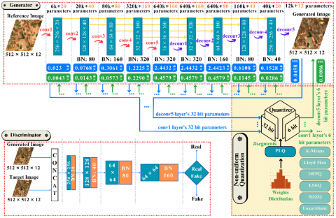
This study builds on the original architecture introduced in MultiTempGAN [13], which utilizes a GAN to compress multitemporal MS images by leveraging temporal redundancy. While earlier extensions applied uniform and mixed-precision quantization to reduce the model size, the present study focuses on improving compression efficiency through post-training NUQ. The goal is to significantly reduce the memory footprint and bpp by lowering weight precision without compromising reconstruction quality, as measured by SNR and LMSE. To enable direct comparisons, the same generator and discriminator architectures are used, with modifications only in the quantization stage.
A variety of NUQ methods were evaluated at 8-bit and 6-bit precision levels. In cases where the 6-bit configurations produced results comparable to full precision, additional experiments were conducted at 4-bit to explore further compression. The methods considered include logarithmic quantization (LQ), dynamic fixed-point quantization (DFPQ), learned step size quantization (LSSQ), scalar dead zone quantization (SDZQ), Lloyd-Max quantization (LMQ), K-Means quantization (KMQ), and the proposed piecewise linear quantization (PLQ). Further details of these techniques are provided in Section 2.4.
Model performance was evaluated against earlier quantized variants of MultiTempGAN and conventional deep learning baselines such as U-Net, LinkNet, and ResNet. The results guided the selection of PLQ with 6-bit precision as the optimal approach, based on its ability to balance compression and reconstruction fidelity across all three datasets that were utilized in this work. Further implementation details of this method are provided in Section 2.5.
Figure 1. Overall architecture of NUQ-MultiTempGAN using piecewise linear quantization (PLQ) with 6-bit precision
Figure 1 presents the full architecture, including the generator and discriminator pipelines, the quantization module, and the corresponding memory optimizations. The diagram illustrates how the quantization module integrates various non-uniform strategies and how PLQ leverages the model’s weight distribution to determine the optimal number of quantization segments. Memory savings resulting from reduced bit-width representation are also visualized for each parameter layer, emphasizing the effectiveness of the proposed approach in minimizing storage without sacrificing reconstruction quality.
2.4 Non-uniform quantization methods
In general, NUQ methods offer a more flexible approach to model compression by assigning varying bit widths to different parts of the model, allowing for a more efficient representation of data while maintaining performance. To identify the most effective NUQ method for post-training quantization, we evaluated several approaches as follows.
LQ uses logarithmically spaced levels to compress larger values while preserving detail for smaller ones [23], whereas DFPQ dynamically adjusts fixed-point representations per layer [24]. LSSQ trains step sizes during training to minimize reconstruction errors [25], while scalar dead zone quantization (SDZQ) introduces a dead zone around zero to better handle sparse weights [26]. Lloyd-Max quantization (LMQ) iteratively minimizes distortion by optimizing quantization levels and boundaries for Gaussian or uniform distributions [27, 28]. K-Means quantization (KMQ) applies clustering to group similar weights in high-dimensional weight spaces [29]. Finally, piecewise linear quantization (PLQ) segments the data range to approximate non-linear distributions using multiple linear pieces [30].
Quantizing models introduces additional parameters, referred to as side information, such as scaling factors and zero points, which are essential for reconstructing the original values during dequantization. Although relatively small, the presence of side information slightly increases the bpp value. Therefore, the bpp after quantization is computed as:
$\mathrm{bpp}=\frac{\text { #q_params } \times \text { bit_precision }+ \text { #nq_params } \times 32+\text { #side_info_params } \times 32}{\text { #pixels } \times \text { #images }}$ (1)
where, #q_params represents the number of quantized parameters stored at reduced precision denoted by bit_precision, while #nq_params and #side_info_params represent the number of non-quantized parameters and side information parameters, both of which are stored at full 32-bit precision.
2.5 Proposed method: Non-uniform quantization with piecewise linear quantization
PLQ is a post-training NUQ approach that adapts the quantization resolution to the empirical distribution of model weights by partitioning the weight range into multiple segments and applying quantization within each segment. Unlike global uniform quantization, which uses a single step size over the entire range, PLQ assigns finer effective resolution to dense regions of the weight distribution (typically concentrated near zero) and coarser resolution to sparse tail regions. This behavior is well suited to pretrained deep neural networks (DNNs) [30], whose weights are commonly highly concentrated around zero with long tails, and therefore benefit from piecewise treatment rather than a single global quantizer. The number of segments is selected to balance approximation accuracy and overhead. In this implementation the number of segments denoted as $N_{\text {segments }}$ is determined by the following lightweight statistics-based heuristic.
$N_{\text{segments}}=\max(2,\lfloor \text{base_scale}+\text{variability_scale}\log_{10}(\frac{w_{\max}-w_{\min}}{\sigma+\epsilon}+1)\rfloor)$ (2)
where, $w_{\max }$ and $w_{\min}$ denote the maximum and minimum weight values, $\sigma$ is the standard deviation, and $\epsilon=1 \times 10^{-8}$ avoids division by zero. The ratio $\left(w_{\text {max }}-w_{\text {min }}\right) /(\sigma+\epsilon)$ acts as a compact proxy for distribution spread and tailheaviness, while the logarithm stabilizes the segment growth against outliers. The constants base_scale = 1.5 and variability_scale = 2.0 were selected experimentally to ensure at least two segments for narrow distributions and increased segmentation for broader/heavier-tailed ones. Alternative segment-selection rules, including a fixed segment count (Fixed- $N$) and a standard-deviation-based ($\sigma$-threshold) heuristic were also evaluated. However, across the evaluated datasets, Eq. (2) consistently produced the best (or near-best) rate-distortion trade-off.
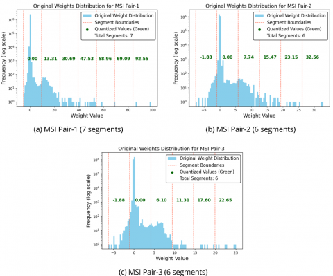
In practice, MSI Pair-1 exhibits a broader, more dispersed weight distribution than MSI Pair-2 and MSI Pair-3, resulting in one additional segment (7 vs. 6). After segmentation, weights are quantized within each segment, providing finer resolution in dense regions and reducing sensitivity to tail outliers. Quantization introduces additional parameters, referred to as side information, that are required for dequantization, such as scales, zero points, segment boundaries, and related quantization metadata. Since defining N segments requires N + 1 boundaries and we quantize 36 generator variables, the total number of side-information parameters is calculated using Eq. (3) resulting in 36 × (7+1) = 288 parameters for the MSI Pair-1 dataset, and 36 × (6+1) = 252 for the MSI Pair-2 and MSI Pair-3 datasets. Figure 2 shows the distribution of the model weights and the corresponding PLQ segment boundaries for each dataset, illustrating how the segment counts adapt based on the characteristics of weight variability.
$\text{#side_information} =N_{\text {quantized_variables }} \times\left(N_{\text {segments }}+1\right)$ (3)
Figure 2. Visualization of the original weight distributions and piecewise linear quantization (PLQ) segment boundaries for each dataset. Segment counts vary depending on the statistical properties of the distribution
The proposed model was evaluated against traditional deep learning-based approaches, as well as the results of the best performing uniform, mixed-precision, and NUQ methods. Table 2 summarizes the results, highlighting trade-offs in bit precision, memory usage, and reconstruction quality, where SNR, LMSE, and structural similarity index measure (SSIM) are averaged across all three datasets for each method.
Quantization methods can be categorized into three main groups: uniform, mixed-precision, and non-uniform. Uniform quantization applies a fixed bit precision across all layers, with variants such as stochastic quantization, which introduces randomness to reduce bias, and symmetric quantization, where values are symmetrically mapped around zero [31]. Mixed-precision quantization assigns different bit depths to different layers to balance efficiency and accuracy, while NUQ adapts to the data distribution for optimized representation.
It is evident from Table 2 that the proposed model significantly outperforms Q-MultiTempGAN. Specifically, it improves the average SNR by approximately 1.7% (from 25.78 to 26.22), reduces the average LMSE by 27.8% (from 0.72 to 0.52), improves the average SSIM by 0.6% (from 0.957 to 0.963), and reduces both memory usage and bit rate by 25% (from 2.44 MB to 1.83 MB and from 0.0148 bpp to 0.0111 bpp, respectively). These results underscore the effectiveness of the proposed quantization scheme in balancing compression efficiency and reconstruction fidelity. To avoid ambiguity, Q-MultiTempGAN is used directly instead of “Symmetric 8-bit” in Table 2 and the figures, since the proposed model in Q-MultiTempGAN utilizes 8-bit uniform symmetric quantization.
The reason for not selecting PLQ with 8-bit precision, despite its average SNR of 26.35 dB and LMSE of 0.40 being nearly identical to those of the original MultiTempGAN model with 26.34 dB and 0.39 respectively, lies in the priority of maximizing compression efficiency. While the 8-bit version provides excellent fidelity, the 6-bit PLQ variant achieves a notably lower bpp of 0.0111 compared to 0.0148 and a higher compression ratio of 5.33 compared to 3.99, with only a minimal reduction in SNR at 26.22 dB, a slightly higher LMSE at 0.52, and a negligible drop in SSIM from 0.965 to 0.963. These quality differences are minor when weighed against the substantial gains in memory savings and transmission cost, which makes the 6-bit PLQ the preferred choice in this study. However, it is important to note that these results are specific to the evaluated datasets and may not generalize across all MS image datasets.
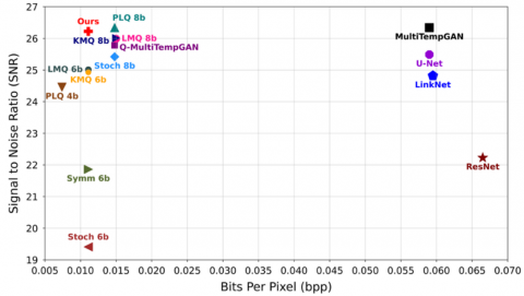
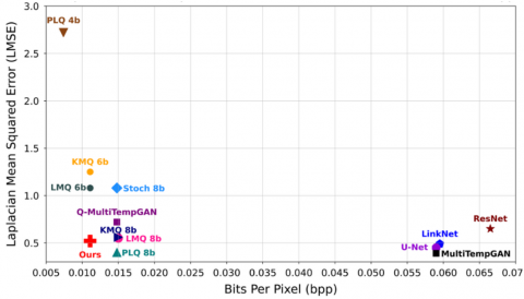
Figure 3 and Figure 4 present a comparative analysis of the proposed model against quantized MultiTempGAN variants and deep learning-based MS image compression models, evaluated in terms of trade-offs between SNR and bpp, as well as LMSE and bpp, respectively. In these plots, symmetric and stochastic quantization methods are denoted as "Symm" and "Stoch", respectively. In Figure 3, models closer to the top left exhibit higher accuracy alongside effective compression, while in Figure 4, models near the bottom left demonstrate better compression and quality.
To complement the averaged SNR and LMSE results in Table 2 and to better reflect remote-sensing–relevant quality aspects, additional metrics were considered for spectral fidelity, structural similarity, and edge/gradient preservation. Specifically, Spectral Angle Mapper (SAM) and Erreur Relative Globale Adimensionnelle de Synthèse (ERGAS) were used to assess spectral fidelity, while Multi-Scale Structural Similarity (MS-SSIM) and Gradient Magnitude Similarity Deviation (GMSD) were used as structure- and edge-sensitive measures. For brevity, these metrics are reported in Table 3 for the deep learning baselines (ResNet, U-Net, LinkNet), the full-precision MultiTempGAN model, Q-MultiTempGAN, and the proposed approach. Since dataset-wise trends were consistent across the remaining methods in Table 2, only these representative models are included to keep the presentation concise while still providing dataset-specific support for the rate–distortion comparisons. It is worth noting that the results in Table 3 are not rounded.
Table 2. Performance comparison of the best quantization approaches and non-quantized models. Layer-wise precision quantization (LWPQ) applies 16-bit precision to critical weights, 8-bit precision to standard weights, and 6-bit precision to weights in non-convolutional layers
|
|
Method |
Bit Precision |
Side Information Parameters |
Memory |
bpp |
SNR |
LMSE |
SSIM |
Ratio |
|
Deep Learning Approaches |
ResNet [13] |
- |
- |
11.00 |
0.0665 |
22.23 |
0.65 |
0.942 |
0.88 |
|
|
U-Net [13] |
- |
- |
9.76 |
0.0590 |
25.49 |
0.45 |
0.962 |
1.00 |
|
LinkNet [13] |
- |
- |
9.84 |
0.0595 |
24.82 |
0.49 |
0.958 |
0.99 |
|
|
MultiTempGAN [13] |
- |
- |
9.76 |
0.0590 |
26.34 |
0.39 |
1.00 |
1.00 |
|
|
Mixed Precision Versions |
Conv Only |
6 |
10 |
1.83 |
0.0111 |
23.93 |
2.41 |
0.932 |
5.31 |
|
Conv Only |
8 |
10 |
2.44 |
0.0148 |
25.19 |
0.66 |
0.956 |
3.98 |
|
|
Non-conv Only |
6 |
26 |
9.76 |
0.059 |
21.44 |
0.40 |
0.944 |
1.0 |
|
|
Non-conv Only |
8 |
26 |
9.76 |
0.059 |
21.47 |
0.40 |
0.945 |
1.0 |
|
|
LWPQ |
16-8-6 |
36 |
2.45 |
0.0147 |
24.93 |
0.57 |
0.958 |
3.97 |
|
|
Uniformly Quantized Versions |
Stochastic |
6 |
36 |
1.83 |
0.0111 |
19.41 |
16.51 |
0.800 |
5.33 |
|
Stochastic |
8 |
36 |
2.44 |
0.0148 |
25.42 |
1.08 |
0.952 |
3.99 |
|
|
Symmetric |
6 |
36 |
1.83 |
0.0111 |
21.86 |
6.11 |
0.885 |
5.33 |
|
|
Q-MultiTempGAN |
8 |
36 |
2.44 |
0.0148 |
25.78 |
0.72 |
0.957 |
3.99 |
|
|
Non-uniform Approaches of NUQ-MultiTempGAN |
LQ |
8 |
9288 |
2.47 |
0.015 |
25.12 |
0.43 |
0.962 |
3.94 |
|
DFPQ |
6 |
36 |
1.83 |
0.0111 |
21.86 |
6.11 |
0.885 |
5.33 |
|
|
DFPQ |
8 |
36 |
2.44 |
0.0148 |
25.78 |
0.72 |
0.958 |
3.99 |
|
|
LSSQ |
6 |
36 |
1.83 |
0.0111 |
20.26 |
3.10 |
0.917 |
5.33 |
|
|
LSSQ |
8 |
36 |
2.44 |
0.0148 |
25.64 |
1.00 |
0.957 |
3.99 |
|
|
SDZQ |
6 |
37 |
1.83 |
0.0111 |
24.31 |
0.43 |
0.955 |
5.33 |
|
|
SDZQ |
8 |
37 |
2.44 |
0.0148 |
23.34 |
0.47 |
0.937 |
3.99 |
|
|
LMQ |
6 |
2304 |
1.84 |
0.0111 |
25.01 |
1.08 |
0.953 |
5.30 |
|
|
LMQ |
8 |
9216 |
2.47 |
0.015 |
25.99 |
0.55 |
0.962 |
3.94 |
|
|
KMQ |
6 |
2304 |
1.84 |
0.0111 |
24.93 |
1.25 |
0.951 |
5.30 |
|
|
KMQ |
8 |
9216 |
2.47 |
0.015 |
26.01 |
0.56 |
0.962 |
3.94 |
|
|
PLQ |
4 |
252 |
1.22 |
0.0074 |
24.46 |
2.72 |
0.93 |
7.99 |
|
|
PLQ |
8 |
252 |
2.44 |
0.0148 |
26.35 |
0.40 |
0.965 |
3.99 |
|
|
Ours |
6 |
252 |
1.83 |
0.0111 |
26.22 |
0.52 |
0.963 |
5.33 |
Figure 3. Comparison of the proposed model with others based on SNR and bpp
Figure 4. Comparison of the proposed model with others based on LMSE and bpp
Table 3. Dataset-wise evaluation using spectral, structural, and edge-sensitive quality metrics in addition to SNR and LMSE
|
Method |
Dataset |
SNR ↑ |
LMSE ↓ |
SAM (°) ↓ |
ERGAS ↓ |
MS-SSIM ↑ |
GMSD ↓ |
|
ResNet |
MSI Pair-1 |
23.659828 |
0.718087 |
3.097701 |
8.671499 |
0.972613 |
0.110862 |
|
MSI Pair-2 |
22.108816 |
0.608300 |
3.452288 |
12.359723 |
0.959396 |
0.113193 |
|
|
MSI Pair-3 |
20.944756 |
0.627533 |
3.751010 |
14.005035 |
0.949541 |
0.119634 |
|
|
Avg. |
22.237800 |
0.651307 |
3.433666 |
11.678752 |
0.960517 |
0.114563 |
|
|
U-Net |
MSI Pair-1 |
27.311175 |
0.511405 |
2.162459 |
6.043228 |
0.983637 |
0.085557 |
|
MSI Pair-2 |
24.856770 |
0.406732 |
2.681054 |
9.157932 |
0.975352 |
0.089369 |
|
|
MSI Pair-3 |
24.303266 |
0.432777 |
2.535983 |
9.924824 |
0.969431 |
0.098977 |
|
|
Avg. |
25.490404 |
0.450305 |
2.459832 |
8.375328 |
0.976140 |
0.091301 |
|
|
LinkNet |
MSI Pair-1 |
26.107079 |
0.622579 |
2.498536 |
7.030402 |
0.980602 |
0.096920 |
|
MSI Pair-2 |
24.805783 |
0.413417 |
2.460151 |
9.728663 |
0.972996 |
0.095012 |
|
|
MSI Pair-3 |
23.575115 |
0.444947 |
2.683340 |
10.711043 |
0.966097 |
0.103859 |
|
|
Avg. |
24.829326 |
0.493648 |
2.547342 |
9.156703 |
0.973232 |
0.098597 |
|
|
MultiTempGAN |
MSI Pair-1 |
27.878707 |
0.465964 |
2.045208 |
5.565498 |
0.984751 |
0.082957 |
|
MSI Pair-2 |
26.437641 |
0.328305 |
2.106845 |
7.818108 |
0.979813 |
0.086433 |
|
|
MSI Pair-3 |
24.728879 |
0.398170 |
2.417396 |
9.260298 |
0.970272 |
0.102629 |
|
|
Avg. |
26.348409 |
0.397480 |
2.189816 |
7.547968 |
0.978279 |
0.090673 |
|
|
Q-MultiTempGAN |
MSI Pair-1 |
27.427145 |
0.750615 |
2.218035 |
5.919681 |
0.983896 |
0.083425 |
|
MSI Pair-2 |
25.674135 |
0.659852 |
2.468970 |
8.199659 |
0.978728 |
0.087821 |
|
|
MSI Pair-3 |
24.225369 |
0.779146 |
2.610249 |
9.770145 |
0.969150 |
0.103513 |
|
|
Avg. |
25.775550 |
0.729871 |
2.432418 |
7.963162 |
0.977258 |
0.091586 |
|
|
Ours |
MSI Pair-1 |
27.841624 |
0.571672 |
2.051323 |
5.546181 |
0.984641 |
0.083058 |
|
MSI Pair-2 |
26.233091 |
0.419700 |
2.195035 |
7.876519 |
0.979632 |
0.086657 |
|
|
MSI Pair-3 |
24.608432 |
0.570438 |
2.506596 |
9.356059 |
0.970041 |
0.102849 |
|
|
Avg. |
26.227716 |
0.520603 |
2.250985 |
7.592920 |
0.978105 |
0.090855 |
Figure 3 and Figure 4 present a comparative analysis of the proposed model against quantized MultiTempGAN variants and deep learning-based MS image compression models, evaluated in terms of trade-offs between SNR and bpp, as well as LMSE and bpp, respectively. In these plots, symmetric and stochastic quantization methods are denoted as "Symm" and "Stoch", respectively. In Figure 3, models closer to the top left exhibit higher accuracy alongside effective compression, while in Figure 4, models near the bottom left demonstrate better compression and quality.
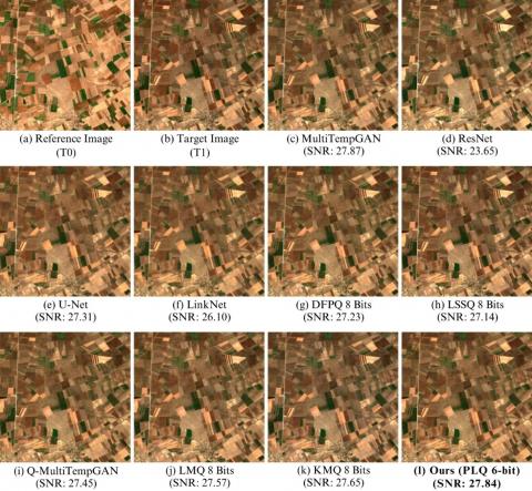
Figure 5 compares the reference, target and generated images produced by various deep learning models and the top performing quantized versions of MultiTempGAN for a randomly selected patch from the MSI Pair-1 dataset. For simplicity and visualization purposes, only the first three spectral channels of the multispectral Sentinel-2 images corresponding to the Red, Green, and Blue (RGB) bands are used. The SNR values shown under each image reflect the specific dataset and approach, not the average across all datasets.
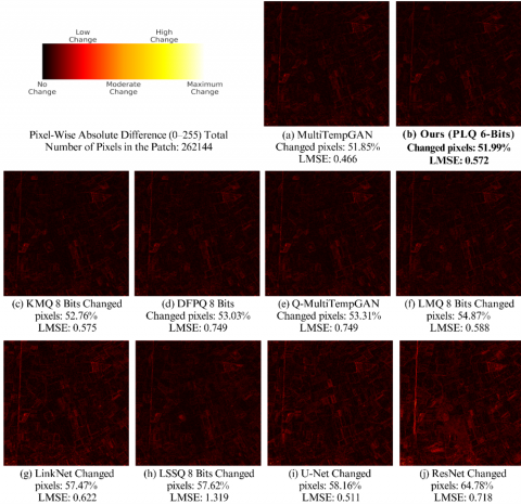
As seen in Figure 5, it is difficult to visually distinguish the differences in images generated by various post-training NUQ techniques with the naked eye. This is mainly because the reconstruction quality of the models is quite similar, and their SNR values do not show significant variation. To provide a more detailed and interpretable comparison, Figure 6 presents heatmaps that illustrate the pixel-wise absolute differences between each reconstructed image and the corresponding target image. These heatmaps were created by comparing the output of each method with the original target image from the same patch in MSI Pair-1 dataset used in Figure 5, which ensures consistency in visual analysis. The percentage of changed pixels shown beneath each heatmap represents the proportion of pixels that differ from the target image, even by a small amount. The LMSE values displayed under each heatmap correspond specifically to this individual patch and dataset and are not averaged values from multiple datasets.
To keep the visualization simple and easy to interpret, only the first three spectral bands corresponding to RGB were used when generating the heatmaps. Before computing the absolute differences, both the reconstructed and target RGB images were converted to grayscale. Each patch is 512 by 512 pixels in size, resulting in 262,144 total pixels in the grayscale image. Since the comparison is performed in grayscale, the pixel count reflects a single-channel image rather than the full three-channel RGB input.
Although the order of models in Figure 6 is based on the percentage of changed pixels from lowest to highest, it does not perfectly match the ranking in Table 2, though the general trend remains consistent. Model performances are not dramatically different, and the heatmaps visually support this observation. For instance, ResNet shows a noticeably higher concentration of yellow regions in the bottom-left corner, aligning with its relatively lower SNR and higher LMSE in Table 2. In contrast, other models show fewer bright yellow or white spots (representing high-magnitude changes) and instead exhibit a gradual increase in red intensity, reflecting the percentage of changed pixels. This progression mirrors the SNR, LMSE, and SSIM patterns in Table 2. The slight differences in order can be attributed to the fact that Table 2 summarizes results averaged over three datasets and all 12 spectral bands, while the heatmaps are based on one randomly selected patch from MSI Pair-1 using only its first three bands converted into a single grayscale image.
Figure 5. Visual comparison of all deep learning-based models, Q-MultiTempGAN, and the top 5 NUQ versions of MultiTempGAN using the best bit precision for each method
Figure 6. Pixel-wise heatmap comparison of all deep learning-based models, Q-MultiTempGAN, and the top 5 NUQ versions of MultiTempGAN using the best bit precision for each method
Efficient compression of MS images is crucial for large-scale remote sensing, where storage and bandwidth constraints are critical. This study introduces NUQ-MultiTempGAN, a non-uniformly quantized version of MultiTempGAN that leverages PLQ to optimize the trade-off between compression and reconstruction quality. Unlike uniform quantization, the proposed approach dynamically adjusts bit precision based on weight distribution, improving compression efficiency while maintaining fidelity.
While applying post-training uniform quantization, specifically 8-bit symmetric quantization, to MultiTempGAN (resulting in Q-MultiTempGAN) produces acceptable results, it is undeniable that all conventional deep learning-based models evaluated in this work, namely U-Net, LinkNet, and ResNet, perform better in terms of average LMSE. Regarding average SSIM, only ResNet ranks below Q-MultiTempGAN. That being said, NUQ-MultiTempGAN not only significantly outperforms all conventional models but also achieves the best performance among all NUQ methods, making it a strong alternative to Q-MultiTempGAN.
The flexibility of this quantization strategy enables dynamic adaptation to different datasets, ensuring scalability across diverse MS images. Although minor adjustments to segmentation parameters may be necessary, this trade-off is minimal compared to the substantial reduction in model size and the gains in computational efficiency. Future work can explore quantization-aware training (QAT) and adaptive mixed-precision strategies to further optimize compression without compromising performance.
[1] Chai, D., Bouzerdoum, A. (2001). Overview of the JPEG2000 image compression standard. In Proceedings of the Seventh Australian and New Zealand Intelligent Information Systems Conference, Perth, WA, Australia. https://doi.org/10.1109/ANZIIS.2001.974083
[2] Fazli, S., Toofan, S., Mehrara, Z. (2012). JPEG2000 image compression using SVM and DWT. International Journal of Science and Engineering Investigations, 1(3): 45-50.
[3] Zhu, W., Du, Q., Fowler, J.E. (2009). Segmented PCA and JPEG2000 for hyperspectral image compression. Satellite Data Compression, Communication, and Processing V, 7455: 118-125. https://doi.org/10.1117/12.825535
[4] Zhang, H., Zhao, E., Ma, L. (2024). Interim connection space based on polynomial models for multispectral image compression and reconstruction. In 2024 International Conference on Image Processing, Computer Vision and Machine Learning (ICICML), Shenzhen, China, pp. 232-236. https://doi.org/10.1109/ICICML63543.2024.10957988
[5] Kaarna, A., Zemcik, P., Kalviainen, H., Parkkinen, J. (1998). Multispectral image compression. In Proceedings Fourteenth International Conference on Pattern Recognition (Cat. No. 98EX170), Brisbane, QLD, Australia, pp. 1264-1267. https://doi.org/10.1109/ICPR.1998.711931
[6] Kong, F., Zhao, S., Li, Y., Li, D. (2021). End-to-end multispectral image compression framework based on adaptive multiscale feature extraction. Journal of Electronic Imaging, 30(1): 013010. https://doi.org/10.1117/1.JEI.30.1.013010
[7] Barman, D., Hasnat, A., Begum, S., Barman, B. (2024). A deep learning based multi-image compression technique. Signal Image Video Processing, 18(Suppl 1): 407-416. https://doi.org/10.1007/s11760-024-03163-8
[8] Anuradha, D., Sekhar, G.C., Mishra, A., Thapar, P., Baker El-Ebiary, Y.A., Syamala, M. (2024). Efficient compression for remote sensing: Multispectral transform and deep recurrent neural networks for lossless hyper-spectral imaging. International Journal of Advanced Computer Science and Applications, 15(2): 531-539. https://doi.org/10.14569/ijacsa.2024.0150256
[9] Yeo, C.K., Soon, I.Y., Lau, C.T. (1999). Lossless compression of multispectral satellite images. Journal of Communications and Networks, 1(4): 226-230. https://doi.org/10.1109/JCN.1999.6597003
[10] Yu, G., Vladimirova, T., Sweeting, M. (2007). A new automatic on-board multispectral image compression system for LEO Earth observation satellites. In 2007 15th International Conference on Digital Signal Processing, Cardiff, UK, pp. 395-398. https://doi.org/10.1109/ICDSP.2007.4288602
[11] Chang, L., Cheng, C.M., Chen, T.C. (2000). An efficient adaptive KLT for multispectral image compression. In 4th IEEE Southwest Symposium on Image Analysis and Interpretation, Austin, TX, USA, pp. 252-255. https://doi.org/10.1109/IAI.2000.839610
[12] Dua, Y., Singh, R.S., Kumar, V. (2022). Compression of multi-temporal hyperspectral images based on RLS filter. Visual Computing, 38(1): 65-75. https://doi.org/10.1007/s00371-020-02000-6
[13] Karaca, A.C., Kara, O., Güllü, M.K. (2021). MultiTempGAN: Multitemporal multispectral image compression framework using generative adversarial networks. Journal of Visual Communication and Image Representation, 81: 103385. https://doi.org/10.1016/j.jvcir.2021.103385
[14] He, K., Zhang, X., Ren, S., Sun, J. (2016). Deep residual learning for image recognition. In Proceedings of the IEEE Conference on Computer Vision and Pattern Recognition (CVPR), Las Vegas, NV, USA, pp. 770-778. https://doi.org/10.1109/CVPR.2016.90
[15] Ronneberger, O., Fischer, P., Brox, T. (2015). U-Net: Convolutional networks for biomedical image segmentation. arXiv:1505.04597. https://doi.org/10.48550/arXiv.1505.04597
[16] Chaurasia, A., Culurciello, E. (2017). LinkNet: Exploiting encoder representations for efficient semantic segmentation. In 2017 IEEE Visual Communications and Image Processing (VCIP), St. Petersburg, FL, USA, pp. 1-4. https://doi.org/10.1109/VCIP.2017.8305148
[17] Isola, P., Zhu, J.-Y., Zhou, T., Efros, A.A. (2018). Image-to-image translation with conditional adversarial networks. IEEE Transactions on Pattern Analysis and Machine Intelligence, 41(11): 2681-2694. https://doi.org/10.1109/TPAMI.2018.2866149
[18] Gharagoz, N.S., Karaca, A.C. (2025). Q-MultiTempGAN: Post-training quantization of multitemporal multispectral image compression models. Applied Computational Engineering, 100(1): 154-162. https://doi.org/10.54254/2755-2721/2025.20699
[19] Ge, Z., Ma, S., Gao, W., Pan, J., Jia, C. (2024). NLIC: Non-uniform quantization-based learned image compression. IEEE Transactions on Circuits and Systems for Video Technology, 34(10): 9647-9663. https://doi.org/10.1109/TCSVT.2024.3401872
[20] Shi, J., Lu, M., Ma, Z. (2024). Rate-distortion optimized post-training quantization for learned image compression. IEEE Transactions on Circuits and Systems for Video Technology, 34(5): 3082-3095. https://doi.org/10.1109/TCSVT.2023.3323015
[21] European Space Agency. SNAP download. https://step.esa.int/main/download/snap-download/, accessed on Feb. 10, 2025.
[22] Copernicus. Copernicus Data Space Browser. https://browser.dataspace.copernicus.eu/, accessed on Feb. 10, 2024.
[23] Van Ess, D. AN2095 algorithm — Logarithmic signal companding: Not just a good idea — It is μ-law. Infineon Application Note AN2095. https://www.infineon.com/.
[24] Kummer, L., Sidak, K., Reichmann, T., Gansterer, W. (2023). Adaptive precision training (AdaPT): A dynamic quantized training approach for DNNs. In Proceedings of the 2023 SIAM International Conference on Data Mining (SDM), pp. 559-567. https://doi.org/10.1137/1.9781611977653.ch63
[25] Esser, S.K., McKinstry, J.L., Bablani, D., Appuswamy, R., Modha, D.S. (2020). Learned step size quantization. arXiv:1912.01309. https://doi.org/10.48550/arXiv.1912.01309
[26] Yu, J. (2004). Advantages of uniform scalar dead-zone quantization in image coding system. In 2004 International Conference on Communications, Circuits and Systems (IEEE Cat. No. 04EX914), Chengdu, China, pp. 805-808. https://doi.org/10.1109/ICCCAS.2004.1346303
[27] Lloyd, S. (1982). Least squares quantization in PCM. IEEE Transactions on Information Theory, 28(2): 129-137. https://doi.org/10.1109/TIT.1982.1056489
[28] Max, J. (1960). Quantizing for minimum distortion. IRE Transactions on Information Theory, 6(1): 7-12. https://doi.org/10.1109/TIT.1960.1057548
[29] Wang, L., Chen, H., Wu, Y. (2017). Compressing deep convolutional networks using K-means based on weights distribution. In Proceedings of the 2nd International Conference on Intelligent Information Processing (ICIIP ’17), Bangkok Thailand, pp. 1-6. https://doi.org/10.1145/3144789.3144803
[30] Fang, J., Shafiee, A., Abdel-Aziz, H., Thorsley, D., Georgiadis, G., Hassoun, J.H. (2020). Post-training piecewise linear quantization for deep neural networks. In European Conference on Computer Vision, pp. 69-86. https://doi.org/10.1007/978-3-030-58536-5_5
[31] Krishnamoorthi, R. (2018). Quantizing deep convolutional networks for efficient inference: A whitepaper. arXiv:1806.08342. https://doi.org/10.48550/arXiv.1806.08342