Adel Dahdouh*![]() | Lakhdar Mazouz
| Lakhdar Mazouz![]() | Ahmed Elottri
| Ahmed Elottri![]() | Brahim Elkhalil Youcefa
| Brahim Elkhalil Youcefa![]()
© 2023 IIETA. This article is published by IIETA and is licensed under the CC BY 4.0 license (http://creativecommons.org/licenses/by/4.0/).
OPEN ACCESS
An innovative methodology for harmonic voltage identification has been introduced, leveraging the application of a multivariable-filter (FMV) to the three-level unified power quality conditioner (UPQC). The UPQC is controlled using a feedback linearization method founded on the space vector modulation (SVM) approach. The main attributes of this novel technique are its simplicity, robustness, and ease of implementation. It necessitates only a Concordia transformation block and an FMV filter. To enhance the performance of the UPQC system, this technique is incorporated into the control strategy. This integration considers an energy minimization based balancing of DC capacitor voltages. A prime advantage of this methodology is the provision of compensation signals with impeccable accuracy and typical speed. This is achievable under a myriad of load conditions, enabling the elimination of current and voltage harmonics while maintaining a high dynamic response. Validation of the proposed method's performance is achieved through MATLAB/Simulink simulations, applied to a diverse nonlinear load. When contrasted with results obtained from the conventional PQ-theory, these simulations demonstrate the superior effectiveness of this newly proposed identification technique.
harmonic voltage identification, multivariable filter, unified power quality conditioner (UPQC), space vector modulation, feedback linearization control
Due to the increased usage of power electronic equipment in recent years, power quality has been decreased due to harmonic generation [1]. Several attempts have been made to determine the standards and classification in IEEE-519 and IEC-555. However, according to these regulations [2], the overall harmonic distortion permitted must be less than 5%.
Passive filters [3] can be used to partially resolve this problem. However, unanticipated instabilities in the load current and voltage wave forms would not be resolved by this type of filter. On the other hand, there is a recommendation that an indemnification device be used in order to obtain good power quality, such as Parallel Active-Filter (PAF), Static Var-Compensator (SVC), hybrid filters and Series Active-Filter (SAF) [4]. Nevertheless, since they can only fix one or two power quality problem, their abilities are usually limited. Previous works have reported that combined conditioners of power quality, which consist of active filters in their two branches, can try to solve the plurality of problems of power quality [5].
There is a UPQC can conserve the load end-voltage constant and prohibit voltage droop/hugeness of entering the system [6]. Furthermore, the UPQC proved efficaciously to deliver the load's reactive power necessities and quell generated harmonic currents, prohibition them from growing back to the efficacy, provoking deformation of voltage and current to another client [7].
Diverse harmonic extraction methods are found. Mahdi and Gorel [8] have implemented a Circuit Constants Based approach. The non-active power parameters for harmonic source detection are suggested by Devassy and Singh [9]. An intelligent extraction method has been applied by Yu et al. [10]. A four-wire UPQC using p-q-r theory has been examined by da Silva et al. [11].
This article includes two goals. Firstly, to develop a new multi-variable based harmonic voltage extraction technique. Compared to other techniques, the proposed multivariable filter methodcharacterized by its simplicity of implementation, and its robustness.
Secondly, to design feedback linearization-based SVM controller with balancing DC Capacitor voltages by using energy minimization approach and compare the suggested technique's performance to that of classic PQ theory to validate the proposed technique by a diverse result for a nonlinear load.
The control technique functioning of the UPQC is presented in Figure 1 in which it is related to a nonlinear load. The operation is based on the switch control signals generation offered by a three-level Space Vector Modulator. The voltage references are offered to the SVM by the feedback linearization controllers. In order to find the harmonic references, the theories of instantaneous PQ and FMV-PQ are utilized for the currents and for the voltages, the FMV-PLL and PQ-PLL methods are used respectively [12-14].
2.1 Mathematical model of GPV-UPQC
In order to achieve effective control over our system, the development of a robust and accurate mathematical model is of utmost importance. By formulating a mathematical of the system, we can gain a deep understanding of its underlying dynamics, behavior, and interconnections. This model serves as a foundation for designing and implementing control strategies that can optimize system performance, enhance stability, and achieve desired objectives.
Figure 1. Feedback linearisation-based SVM control scheme of the UPQC
Eq. (1) and Eq. (3) in α-β stationary frame illustrate the dynamic model of the UPQC’s. The following equations present the model of parallel filter:
$\begin{aligned} & \frac{d i_{f p \alpha}}{d t}=-\frac{R_{f p}}{L_{f p}} i_{f p \alpha}-\frac{v_{s \alpha}}{L_{f p}}+\frac{v_{f p \alpha}}{L_{f p}} \\ & \frac{d i_{f p \beta}}{d t}=-\frac{R_{f p}}{L_{f p}} i_{f p \beta}-\frac{v_{s \beta}}{L_{f p}}+\frac{v_{f p \beta}}{L_{f p}}\end{aligned}$ (1)
and
$\dot{x}_p=f_p\left(x_p\right)+g_p\left(x_p\right) u_p$ (2)
where,
$\begin{gathered}f_p\left(x_p\right)=\left[\begin{array}{c}-\frac{R_{f p}}{L_{f p}} i_{f p \alpha}-\frac{v_{s \alpha}}{L_{f p}} \\ -\frac{R_{f p}}{L_{f p}} i_{f p \beta}-\frac{v_{s \beta}}{L_{f p}}\end{array}\right], g_p\left(x_p\right)=\left[\begin{array}{cc}\frac{1}{L_{f p}} & 0 \\ 0 & \frac{1}{L_{f p}}\end{array}\right] \\ x_p=\left[\begin{array}{c}i_{f p \alpha} \\ i_{f p \beta}\end{array}\right], u_p=\left[\begin{array}{c}v_{f p \alpha} \\ v_{f p \beta}\end{array}\right]\end{gathered}$
ifpαβ and vfpαβ present the currents and voltages of the shunt filter and vsαβ are the voltages.
Model of series filter is given:
$\begin{aligned} & \frac{d i_{f s \alpha}}{d t}=-\frac{R_{f s}}{L_{f s}} i_{f s \alpha}-\frac{v_{i n j \alpha}}{L_{f s}}+\frac{v_{f s \alpha}}{L_{f s}} \\ & \frac{d i_{f s \beta}}{d t}=-\frac{R_{f p}}{L_{f s}} i_{f s \beta}-\frac{v_{i n j \beta}}{L_{f s}}+\frac{v_{f s \beta}}{L_{f s}}\end{aligned}$ (3)
Eq. (3) is given by:
$\dot{x}_s=f_s\left(x_s\right)+g_s\left(x_s\right) u_s$ (4)
in which,
$\begin{gathered}f_s\left(x_s\right)=\left[\begin{array}{c}-\frac{R_{f s}}{L_{f s}} i_{f s \alpha}-\frac{v_{i n j \alpha}}{L_{f s}} \\ -\frac{R_{f s}}{L_{f s}} i_{f s \beta}-\frac{v_{i n j \beta}}{L_{f s s}}\end{array}\right], g_s\left(x_s\right)=\left[\begin{array}{cc}\frac{1}{L_{f s}} & 0 \\ 0 & \frac{1}{L_{f s}}\end{array}\right] \\ x_s=\left[\begin{array}{l}i_{f s \alpha} \\ i_{f s \beta}\end{array}\right], u_s=\left[\begin{array}{l}v_{f s \alpha} \\ v_{f s \beta}\end{array}\right], y_s=\left[\begin{array}{l}y_{s 1} \\ y_{s 2}\end{array}\right]=\left[\begin{array}{l}h_{s 1} \\ h_{s 2}\end{array}\right]\end{gathered}$
where, vfsαβ: voltages, ifsαβ: the α-β axis currents and vinjαβ: the injected voltages in the α-β coordinates of series filter.
The DC-Bus is modelled as follows:
$\frac{d v_{d c}^2}{d t}=\frac{2 P_c}{C_{d k}}$ (5)
and
$\dot{x}_{d c}=f_{d c}\left(x_{d c}\right)+g_{d c}\left(x_{d c}\right) u_{d c}$ (6)
where, $f_{d c}\left(x_{d c}\right)=0, g_{d c}\left(x_{d c}\right)=\frac{2}{c_{d c}}$ and $u_{d c}\left(x_{d c}\right)=P_c$.
2.2 Classification of harmonicextraction methods
The active filter performance should be improved and that passes by identify an applied strategy in order to eliminate harmonics caused by disturbed waveforms [7, 14]. These strategies are well detailed in the following sections.
2.2.1 Muti-variable filter
Multi-Variable Filter FMV is based on the Song Hong-Scok functioning in which the fundamental signals extraction is done directly from the axes (αβ) [6].
On the other hand, this filter can be used to separate a particular harmonics order in its direct or inverse form. the following equation gives the integration equivalent transfer function in the synchronous references frame:
$H(s)=\frac{V_{x y}\quad(s)}{U_{x y}\quad(s)}=\frac{s+j \omega}{s^2+\omega^2}$ (7)
It is clear from this transfer that the output signal is in phase with the input one, caused by the integration effect of the amplitude. In addition, the Bode diagram shows that the effect of this transfer function is similar to a bandpass filter. If constants k1 and k2 are added to the previous transfer, the following equation can be obtained:
$H(s)=\frac{V_{x y}(s)}{U_{x y}(s)}=k_2 \frac{\left(s+k_1\right)+j \omega}{\left(s+k_1\right)^2+\omega^2}$ (8)
The choice of k1 = k2 = k is necessary to obtain (H(s)=0dB) and a zero-phase shift angle between input and output, the transfer function becomes:
$H(s)=\frac{V_{x y}(s)}{U_{x y}(s)}=k \frac{(s+k)+j \omega}{(s+k)^2+\omega^2}$ (9)
If now $V_{x y}$ by $X_{\alpha \beta}$ and $U_{x y}$ by $\bar{X}_{\alpha \beta}$ are replaced, it can be obtained:
$H(s)=\frac{\bar{X}_\alpha(s)+j \bar{X}_\beta(s)}{X_\alpha(s)+j X_\beta(s)}=k \frac{(s+k)+j \omega}{(s+k)^2+\omega^2}$ (10)
That gives us
$\bar{X}_\alpha(s)=\frac{k}{s}\left[X_\alpha(s)-\bar{X}_\alpha(s)\right]-\frac{\omega}{s} \bar{X}_\beta(s)$ (11)
Similarly, from (10) we find $X_\alpha(s)$:
$\bar{X}_\beta(s)=\frac{k}{s}\left[X_\beta(s)-\bar{X}_\beta(s)\right]+\frac{\omega}{s} \bar{X}_\alpha(s)$ (12)
where,
$X_{\alpha \beta}$ : Input signals in the stationary reference frame;
$\bar{X}_{\alpha \beta}$: Fundamental components of $X_{\alpha \beta}$;
$\omega=2 \pi f_s$: Fundamental pulsatance of $X_{\alpha \beta}$;
k: Constant to be fixed.
Finally, the diagram of this filter is represented by the Figure 2.
Figure 2. FMV schematic diagram
2.2.2 Classification of harmonic currents extraction methods
(a) PQ-theory
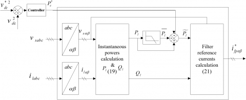
In this section, The common technique of the instantaneous power theory PQ (Figure 3) is explained.
Figure 3. Diagram of PQ technique for extracting of harmonic currents
The following equation presents the powers of the load:
$\left[\begin{array}{l}P_l \\ Q_l\end{array}\right]=\left[\begin{array}{cc}v_{s \alpha} & v_{s \beta} \\ v_{s \beta} & -v_{s \alpha}\end{array}\right]\left[\begin{array}{l}i_{l \alpha} \\ i_{l \beta}\end{array}\right]$ (13)
Also,
$\left\{\begin{array}{l}P_l=\bar{P}_l+\tilde{P}_l \\ Q_l=\bar{Q}_l+\tilde{Q}_l\end{array}\right.$ (14)
In order to compensate reactive power and also to extenuate harmonics, the reactive power components and the active power component are selected as references of compensatory power, next, the reference for currents compensation are computed by:
$\left[\begin{array}{c}i_{f p \alpha}^* \\ i_{f p \beta}^*\end{array}\right]=\frac{1}{v_{s \alpha}^2+v_{s \beta}^2}\left[\begin{array}{cc}v_{s \alpha} & v_{s \beta} \\ v_{s \beta} & -v_{s \alpha}\end{array}\right]\left[\begin{array}{l}\tilde{P}_l \\ Q_l\end{array}\right]$ (15)
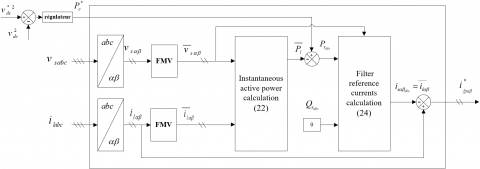
(b) FMV-PQ theory
The Concordia transformation reduces the three-phase system of voltages and currents to a two-phase system of voltages and currents. The FMVs used at the level of voltages and currents, allows filtering efficiently their harmonic components.
The DC component of the active power can be calculated by:
$\bar{P}_l=\bar{v}_{s \alpha} \bar{i}_{l \alpha}+\bar{v}_{s \beta} \bar{i}_{l \beta}$ (16)
The active power that the source must provide expressed as follows:
$P_{s_{d c s}}=-\overline{P_l}+P_c$ (17)
The reactive power of the source is imposed as zero ($Q_{s_{\text {des }}}=0$). The fundamental currents in the stationary reference frame are calculated by:
$\left[\begin{array}{l}i_{s \alpha_{d e s}} \\ i_{s \beta_{d s}}\end{array}\right]=\left[\begin{array}{l}\bar{i}_{l \alpha} \\ \bar{i}_{l \beta}\end{array}\right]=\frac{1}{\bar{v}_{s \alpha}^2+\bar{v}_{s \beta}^2}\left[\begin{array}{ll}\bar{v}_{s \alpha} & \bar{v}_{s \beta} \\ \bar{v}_{s \beta} & -\bar{v}_{s \alpha}\end{array}\right]\left[\begin{array}{l}P_{s d e s} \\ 0\end{array}\right]$ (18)
Finally, the reference harmonic currents in the stationary reference frame are calculated by:
$i_{f p \alpha \beta}^*=i_{\alpha \alpha \beta}-\bar{i}_{l \alpha \beta}$ (19)
Figure 4 depicts the schematic diagram of the FMV-PQ method, while Figure 5 shows the schematic diagram of the PQ-PLL technique.
Figure 4. Diagram of FMV-PQ technique for extracting of harmonic currents
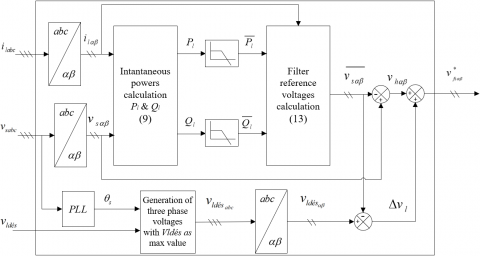
Figure 5. Extracting of harmonic voltages with PQ-PLL technique
2.2.3 Classification of harmonic voltages extraction methods
(a) PQ-PLLtechnique
First, this method extracts voltage harmonics, as presented in Eq. (20).
$\left[\begin{array}{l}\overline{v_{s \alpha}} \\ \overline{v_{s \beta}}\end{array}\right]$= $\frac{1}{i_{l \alpha}^2+i_{l \beta}^2}\left[\begin{array}{cc}i_{l \alpha} & i_{l \beta} \\ -i_{l \beta} & i_{l \alpha}\end{array}\right]\left[\begin{array}{l}\bar{P}_l \\ \overline{Q_l}\end{array}\right]$ (20)
The harmonic voltages are calculated by:
$\left[\begin{array}{c}v_{h \alpha} \\ v_{h \beta}\end{array}\right]=\left[\begin{array}{l}v_{s \alpha} \\ v_{s \beta}\end{array}\right]-\left[\begin{array}{l}\overline{v_{s \alpha}} \\ \overline{v_{s \beta}}\end{array}\right]$ (21)
The reference voltages are presented in Eq. (22) and this can be obtained by adding the voltage drop through the load:
$\left[\begin{array}{c}v_{f s \alpha}^* \\ v_{f s \beta}^*\end{array}\right]=\left[\begin{array}{l}v_{h \alpha} \\ v_{h \beta}\end{array}\right]+\left[\begin{array}{l}\Delta v_{l \alpha} \\ \Delta v_{l \beta}\end{array}\right]$ (22)
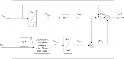
(b) FMV-PLL theory
The proposed method in this article is a new method qualified by its simplicity of implementation, and its robustness. Indeed, it only requires a Concordia transformation block and an FMV. So, by passing the perturbed voltage expressed in (α-β) reference frame through a multivariable filter (FMV) with a sub tractor, the harmonic voltages is simply obtained, and by adding the voltage drop of the load (common part), the schematic diagram of this method is illustrated by Figure 6.
2.3 Synthesis of feedback linearization controller
Eq. (23) presents a nonlinear system in which f(x), h(x) and g(x) are scalar functions:
$x=f(x)+\sum_{i=1}^p g_i(x) u_i, y_i=h_i(x) \quad i=1,2, \ldots, p$ (23)
f(x), h(x) and g(x) represent a scalar functions.
Figure 6. Diagram of FMV- PLL technique for extracting of Harmonic voltages
The feedback linearization law of the system in Eq. (23) is well presented in Figure 5 [15]. to establish the relative degree of the system vector Eq. (13) which requires the separation of each output signal until one of the input signals is clearly integrated in the differentiation.
In $y_i^{\left(r_j\right)}$ is defined as the minimal integer [6]:
$y_j^{\left(r_j\right)}=L_f^{r_j} h(x)+\sum_{i=1}^p L_{g i}\left(L_f^{r_j-1} h_j(x)\right) u_i \quad j=1,2, \ldots \ldots, p$ (24)
where, $L_f h_j$ and $L_{g i}\left(L_f^{r_j^{-1}} h_j\right)$ signify the derivatives of h with respect to f and g.
By using Eq. (24), The total relative degree equals to computed all relative degrees. This relative degree must be less than or equal to the system's order: $r=\sum_{j=1}^p r_j \leq n$.
In order to get the linearising law expression, the Eq. (24) in its matrix form can used and makes the link between inputs and outputs linear:
$\left[\begin{array}{llll}y_1^{r_j} & \ldots & \ldots & y_p^{r_p}\end{array}\right]^t=\zeta(x)+D(x) u$ (25)
where,
$u=D(x)^{-1}(-\zeta(x)+v)$ (26)
U is law of the linearizing control.
The linearization can be obtained if only the decoupling matrix D(x) is reversible.
2.3.1 DC-link voltage FLC design
Based on Eq. (6), The controller of DC link voltage configuration can be obtained. The output derivative $y=h v_{d c}^2$ can be calculated:
$\dot{y}=L_f h(x)+L_g h(x) u=\frac{2}{C_{d c}} P_{d c}$ (27)
The relative degree r of the control Pdc is equal to 1. this output relative degree is equal to the system order and this obviously corresponding to an accurate linearisation [7].
The control can be given:
$P_{d c}^*=\frac{C_{d c}}{2} v$ (28)
where, $\dot{y}=v$.
$v_{d c}^*(t)$ dentified course tracking problem, so the law of linearizing regulation v is described by:
$v=k_{d c}\left(v_{d c}^{* 2}-v_{d c}^2\right)+\frac{d v_{d c}^{* 2}}{d t}$ (29)
where, kdc is aconstant.
2.3.2 Parallel currents FLC design
The Eq. (2) is transformed to the following matrix:
$\left[\begin{array}{l}\dot{y}_{p 1} \\ \dot{y}_{p 2}\end{array}\right]=\left[\begin{array}{l}-\frac{R_{f p}}{L_{f p}} x_{p 1} \\ -\frac{R_{f p}}{L_{f p}} x_{p 2}\end{array}\right]+\left[\begin{array}{cc}\frac{1}{L_{f p}} & 0 \\ 0 & \frac{1}{L_{f p}}\end{array}\right]\left[\begin{array}{l}u_{p 1} \\ u_{p 2}\end{array}\right]$ (30)
By applicating the linearisation law, the regulation law can be obtained by:
$\begin{aligned} & v_{f p \alpha}^*=R_{f p} i_{f p \alpha}+v_{s \alpha}+L_{f p}\left(k_{p 1}\left(i_{f p \alpha}^*-i_{f p \alpha}\right)+\frac{d i_{f p \alpha}^*}{d t}\right) \\ & v_{f p \beta}^*=R_{f p} i_{f p \beta}+v_{s \beta}+L_{f p}\left(k_{p 2}\left(i_{f p \beta}^*-i_{f p \beta}\right)+\frac{d i_{f p \beta}^*}{d t}\right)\end{aligned}$ (31)
2.3.3 Series currents FLC design
The Eq. (4) can be written in the matrix form as:
$\left[\begin{array}{l}\dot{y}_{s 1} \\ \dot{y}_{s 2}\end{array}\right]=\left[\begin{array}{l}-\frac{R_{f s}}{L_{f s}} x_{s 1} \\ -\frac{R_{f s}}{L_{f s}} x_{s 2}\end{array}\right]+\left[\begin{array}{cc}\frac{1}{L_{f s}} & 0 \\ 0 & \frac{1}{L_{f s}}\end{array}\right]\left[\begin{array}{l}u_{s 1} \\ u_{s 2}\end{array}\right]$ (32)
Using Eq. (25) and Eq. (26), the regulation law can be obtained by:
$\begin{aligned} & v_{f s \alpha}^*=R_{f s} i_{f s \alpha}+v_{i n j \alpha}+L_{f s}\left(k_{s 1}\left(i_{f s \alpha}^*-i_{f s \alpha}\right)+\frac{d i_{f s \alpha}^*}{d t}\right) \\ & v_{f s \beta}^*=R_{f s} i_{f s \beta}+v_{i n j \beta}+L_{f s}\left(k_{s 2}\left(i_{f s \beta}^*-i_{f s \beta}\right)+\frac{d i_{f s \beta}^*}{d t}\right)\end{aligned}$ (33)
Figure 7. Linearised system configuration
2.4 Three-level space vector modulator
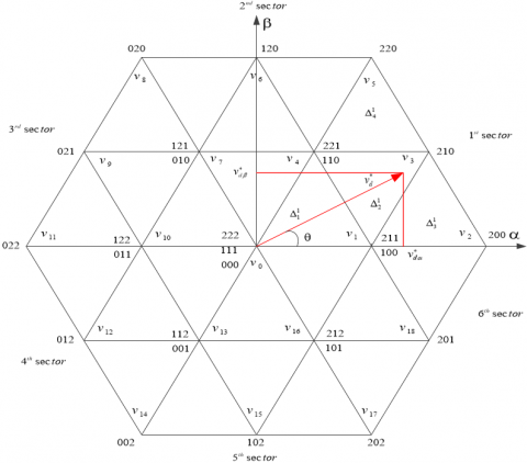
Figure 8. Design of three-level space-vector
Figure 9. Configuration of vector in initial sector
For generating PWM control signals (sa, sb, and sc) of switches, a three-levels SVM algorithm is illustrated. The space vectors given to the three-level inverter in the α-β coordinate system is shown in Figure 7. The space vectors given in the frame of the three-level inverter is given in Figure 8. There are 27 states. 3 zero states in the middle, 12 on the inner hexes and 12 on the outer hexes. For these conditions, '2', '0', and '1' mean that the output voltage can have 'vdc/2', '0', and '-vdc/2' correspondingly.
Each sector consists of four triangular regions, as shown in Figure 9. The objective from the use of space vector modulation is to restructure the reference voltage vector in which that the sum of its three adjacent vectors becomes equal to this reference. Therefore, the first step is to find the reference voltage vector. This first step is to identify the sector number and then to compute the triangle in order to place the vector [15-19].
The reference voltage vector magnitude and also its angle can be defined by:
$v_d^*=\sqrt{v_{d \alpha}^{* 2}+v_{d \beta}^{* 2}}$ (34)
$\theta=\tan 2^{-1}\left(\frac{v_{d \beta}^*}{v_{d \alpha}^*}\right)$ (35)
(a) Determination of sector
The numbers of sector can be obtained by:
$S=\operatorname{ceil}\left(\frac{\theta}{\pi / 3}\right) \in\{1,2,3,4,5,6\}$ (36)
In which ceil is a function in which a number is rounding to the next larger integer.
(b) Triangle identification
The vector of reference is projected on two axes in which there is $\pi / 3_{\mathrm{rad}}$ between them. The projected components can be regularized by:
$\begin{aligned} & v_1^{* S}= 2 \frac{v_d^*}{\sqrt{2 / 3} v_{d c}}\left(\cos \left(\theta-(S-1) \frac{\pi}{3}\right)-\frac{1}{\sqrt{3}} \sin \left(\theta-(S-1) \frac{\pi}{3}\right)\right)\end{aligned}$ (37)
$v_2^{* S}=2 \frac{v_d^*}{\sqrt{2 / 3} v_{d c}}\left(\frac{2}{\sqrt{3}} \sin \left(\theta-(S-1) \frac{\pi}{3}\right)\right)$ (38)
For finding the triangles number in a sector S, it is necessary to define the two integers [20]:
$l_1^S=\operatorname{int}\left(v_1^{* S}\right), l_2^S=\operatorname{int}\left(v_2^{* S}\right)$ (39)
where, int is a function in which a number is rounding to the nearest integer near zero.
To verify the reference vector s situated in the triangle shaped by the vertices K, H and G or in that shaped by the vertices M, K and H, one of the situations should be confirmed [21]:
$v_d^{* S}$ is positioned in GHK triangle if:
$v_1^{* S}+v_2^{* S}<l_1^S+l_2^S+1$ (40)
$v_d^{* S}$ is located in the triangle HKM if:
$v_1^{* S}+v_2^{* S} \geq l_1^S+l_2^S+1$ (41)
With the similar process, the numbers of other triangles in every sector can be determined.
Table 1. Time period in sector s for each triangle
|
Number of Triangle |
Period of Time |
||
|
$t_x^{\Delta_i^S}$ |
$t_y^{\Delta_i^S}$ |
$t_z^{\Delta_i^S}$ |
|
|
$\Delta_1^S(G, H, K)$ |
$T_s-t_y^{\Delta_i^S}-t_z^{\Delta_i^S}$ |
$v_1^{* S} T_S$ |
$v_2^{* S} T_S$ |
|
$\Delta_2^S(M, K, H)$ |
$T_s-t_y^{\Delta_i^S}-t_z^{\Delta_i^S}$ |
$\left(1-v_1^{* S}\right) T_s$ |
$\left(1-v_2^{* S}\right) T_s$ |
|
$\Delta_3^S(H, N, M)$ |
$T_s-t_y^{\Delta_i^S}-t_z^{\Delta_i^S}$ |
$\left(v_1^{* S}-1\right) T_s$ |
$v_2^{* S} T_S$ |
|
$\Delta_4^S(K, M, L)$ |
$T_s-t_y^{\Delta_i^S}-t_z^{\Delta_i^S}$ |
$v_1^{* S} T_S$ |
$\left(v_2^{* S}-1\right) T_s$ |
(c) Duration times calculation
If the reference vector is positioned in HKM triangle, it is restructured from the three neighboring vectors $v_x^{\Delta_i^S}, v_y^{\Delta_i^S}$ and $v_z^{\Delta_i^S}$ using the following relation:
$\begin{gathered}v_x^{\Delta_i^S} t_x^{\Delta_i^S}+v_y^{\Delta_i^S} t_y^{\Delta_i^S}+v_z^{\Delta_i^S} t_z^{\Delta_i^S}=v_d^* T_s \\ t_x^{\Delta_i^S}+t_y^{\Delta_i^S}+t_z^{\Delta_i^S}=T_s\end{gathered}$ (42)
where, $t_x^{\Delta_i^S}, t_y^{\Delta_i^S}$ and $t_z^{\Delta_i^S}$ are the duration times of vectors.
By replacement the coordinates of $v_x, v_y$ and $v_z$, in each triangle, the on-duration time intervals are cited in Table 1.
2.5 Energy minimization based balancing dc capacitor voltages
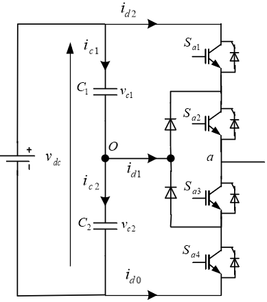
As illustrated in Figure 10, in a three-level diode-clamped converter, the two capacitors total energy is presented in reference [6, 22]:
$E=\frac{1}{2} \sum_{i=1}^2 C_i v_{c i}^2$ (43)
Figure 10. Three-level diode-clamped inverter cell
Assuming that the two capacitors have equal capacitances, C1=C2=C, the total energy E reaches its minimum ($E_{\text {min }}$) when the two capacitors’ voltages are balanced. The minimum total energy is given as follows:
$E_{\min }=\frac{C}{2} \frac{v_{d c}^2}{2}$ (44)
The energy minimization property can be used for capacitor voltages balancing. For this reason, a cost function J is defined based on the quadratic sum of the differences between the voltages $v_{c i}$ and their reference values as follows:
$J=\frac{1}{2} C \sum_{i=2}^{n-1}\left(v_{c i}-\frac{v_{d c}}{2}\right)^2$ (45)
Based on a suitable choice of redundant vectors, the function J can be minimized to zero and the voltages of the capacitors will be maintained at their reference values. The mathematical condition ensuring the convergence of the cost function J to its minimum value is given in:
$\frac{d J}{d t}=\sum_{i=1}^2 \Delta v_{c i} i_{c i} \leq 0$ (46)
where, $i_{c i}$ is the current through capacitor $C_i, i=1,2$.
This investigation of voltage filtering and harmonic current shows, that the compensation and the performance of reactive power evaluation of the multilevel UPQC with the suggested harmonic extraction technique has been analyzed in MATLAB/Simulink underneath variation of nonlinear load and sag/swell of voltage. All system parameters are cited in the following Table 2.
Table 2. System parameters
|
Parameter |
Value |
|
Source voltage for RMS value |
220V |
|
kdc |
250 |
|
The impedance of sours Rs, Ls |
3mΩ, 2.6μH |
|
The frequency of switching fs |
12kHz |
|
The impedances of series filter Rfs, Lfs,Cfs |
1.5Ω, 3mH, 0.1mF |
|
ks1= ks2 |
1150 |
|
The impedances of Line Rl, Ll |
10.0mΩ, 0.3μH |
|
Diode rectifier load Rd , Ld |
15.0Ω, 2mH |
|
The reference of DC-link voltage |
900V |
|
The parameters of Lpv,Cpvboost converter |
5mH, 55mF |
|
kp1= kp2 |
1120 |
|
Photovoltaic generator Ppv, Vmp,Imp, Isc,Voc |
150.0W, 34.5V, 4.35A, 4.75A, 43.5V |
|
The impedance of the shunt filter for (Rfp, Lfp) |
20mΩ, 2.5mH |
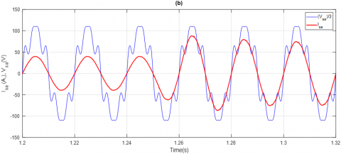
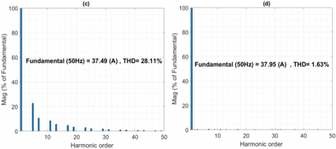
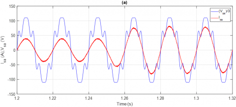
Dynamic demeanor beneath sudden differences in load, by inserting another load including the same value at [t=1.25s] which is explained in Figures 11(a) and (b) in which source voltage and source current of a-phase before compensation and after compensation is presented. It is obvious to notice that the grid current, after using the control, is pure sinusoidal, furthermore, actually, in this transient state, the unity power factor purpose is successfully gained. the proposed technique is well validated in Figures 11(c) and (d) in which the source current harmonic spectrum before and after compensation is proved.
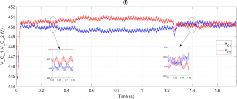
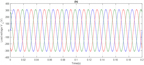
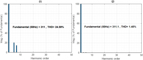
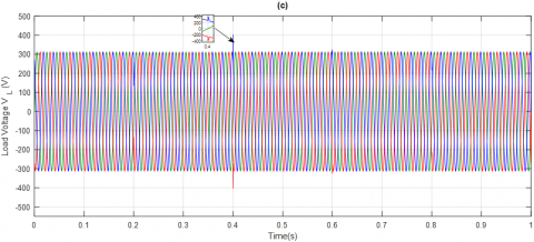
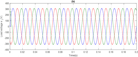
Figure 11. Different results with or under load variation by using the suggested method (FMV): (a) A-phase source voltage with source current before compensation. (b) A-phase source voltage with source current after compensation. (c) Source current harmonic spectrum before compensation. (d) Source current harmonic spectrum after compensation. (e) DC-link voltage vdc. (f) DC capacitors voltages. (g) Voltage of the load before compensation. (h) Harmonic spectrum of load voltage after compensation. (i) Load voltage harmonic spectrum before compensation. (j) Load voltage harmonic spectrum after compensation
The load variation has an insignificant impact about 2V on the voltage of DC-link, and it recuperates about 0.05s as shown Figures 11(e) and (f). it can be seen that the DC capacitors voltages are balancing at their reference values (450 V) with small ripple around the balance point which confirms the effectiveness of the three-level SVM based on a balancing strategy. In Figures 11(g) and (h), the voltage of the load before and after compensation is illustrated and Harmonic spectrum of load voltage before and after compensation is presented in Figures 11(i) and (j) with objective to verify the effectiveness of the suggested method.
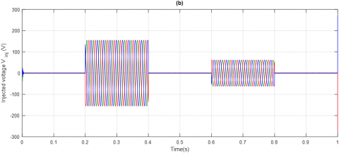
Figures 12(a) and (b) present the voltage of disturbed source and the voltage of compensation under perturbed regime respectively. As shown in these figures, the droop and swell tests it can be regarded that the UPQC fast injects equivalent positive voltage components, in the case of droop which is phase-locked to the grid voltage, while in the case of voltage swell, the UPQC insinuate negative voltage components in the contrasting phase with grid voltage to fix and hold the load voltage near to its regular value as shown in Figure 12(c) in which the voltage of the load after compensation is given.
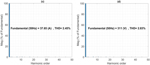
In case of FMV based technique, the study of the load AC grid current spectral with and without compensation and also for voltage are shown in Figures 11(c), (d) and (g) and (h) respectively. In case of PQ-technique, the same spectrums in Figure 13(c) for source current harmonic and in Figure 13(d) for load voltage harmonic are illustrated after compensation respectively. For this method, in one hand Figures 13(a) and (b) show after compensation, the situations of voltages of source and load respectively and in other hand Figures 13(e) and (f) illustrate DC bus voltage vdc and DC capacitors voltages. In classic PQ-theory, the UPQC reduces in the grid, the current THD from 28.11% to 2.45%. However, with FMV based technique, the current THD is reduced to 1.63%. In one hand with PQ-theory, the load voltage THD reduces from 24.59% to 2.83% and in other hand it is reduced to 1.45% in case of FMV technique. It is clear that the later demonstrate the effectiveness of the proposed harmonic extraction technique.
Figure 12. Sag and swell examination of the proposed method: (a) Perturbed source voltage profile. (b) Compensation voltage during perturbation. (c) Voltage of the load after compensation
Figure 13. Simulation results using conventional PQ-theory: (a) A-phase source voltage with source current after compensation. (b) Voltage of the load after compensation. (c) Source current harmonic spectrum after compensation. (d) Load voltage harmonic spectrum after compensation. (e) DC bus voltage vdc
At the voltage of gird the grid voltage, The UPQC is experimented in two situations (sag/swell). As result, the load voltage is quickly obtained very close to a sinusoidal voltage.
Table 3. Comparison of PQ with FMV approaches
|
Factor |
PQ |
FMV |
|
THDv (%) |
2.83 |
1.45 |
|
DC link charging (s) |
0.08 |
0.05 |
|
THDi (%) |
2.45 |
1.63 |
In conclusion, the UPQC is qualified to provide the voltage components of needed compensating to maintain constant the voltage of load. Table 3 shows the FMV-based method quality and efficacy compared to the classic PQ theory, because of an exceed lack in DC bus voltage response through variation of load, quickness and insignificant THD.
In this proposed work, a new technique for harmonic voltage identification based on multivariable-filter applied to three-level unified power quality conditioner controlled by feedback linearization based on space vector modulation (SVM) approach. The new method qualified by its simplicity of implementation, and its robustness., a three-level SVM, considering energy minimization based balancing DC capacitor voltages approach are utilized For switches control because of its advantages as implementation fixed frequency. The obtained results show that during the functioning of system, the currents of source side and the side voltages of load are extremely close to a sinusoidal shape. Compared to the case of conventional PQ-theory, it is obviously that UPQC using the proposed FMV-based technique presents a large amount performance.
|
Xfp |
Xrelated to the parallel filter |
|
Xfs |
Xrelated to the series filter |
|
P Q |
Active Power (W) Reactive Power (VAR) |
|
i |
Electrical Current (A) |
|
v |
Electrical Voltage (V) |
|
GPV |
PhotoVoltaic Generator |
|
UPQC |
Unified Power quality Conditioner |
|
SVM |
Space Vector Modulation |
|
DC |
Direct Current |
|
FL |
Feedback Linearisation |
|
THD |
Total Harmonic Distortion |
[1] Gongati, P.R.R., Marala, R.R., Malupu, V.K. (2020). Mitigation of certain power quality issues in wind energy conversion system using UPQC and IUPQC devices. European Journal of Electrical Engineering, 22(6): 447-455. https://doi.org/10.18280/ejee.220606
[2] Kanchanapalli, B., Vekata, R.R.P.V., Lanka, R.S. (2022). Analysis and comparison of performance of interline power flow controller with various control algorithms under various power stability problems. Traitement du Signal, 39(5): 1605-1613. https://doi.org/10.18280/ts.390517
[3] De Silva, H.J., Shafieipour, M. (2021). An improved passivity enforcement algorithm for transmission line models using passive filters. Electric Power Systems Research, 196: 107255. https://doi.org/10.1016/j.epsr.2021.107255
[4] Bacon, V.D., da Silva, S.A.O., Guerrero, J.M. (2022). Multifunctional UPQC operating as an interface converter between hybrid AC-DC microgrids and utility grids. International Journal of Electrical Power & Energy Systems, 136: 107638. https://doi.org/10.1016/j.ijepes.2021.107638
[5] Dahdouh, A., Mazouz, L., Youcefa, B.E. (2022). Nonlinear predictive direct power control based on space vector modulation of 3-phase 3-level solar PV integrated unified power quality conditioner. European Journal of Electrical Engineering, 24(2): 77-88. https://doi.org/10.18280/ejee.240202
[6] Benaissa, A., Bouzidi, M., Barkat, S. (2012). Application of feedback linearization to the virtual flux direct power control of three-level three-phase shunt active power filter. International Review on Modelling and Simulations, 5(3): 1128-1140. https://doi.org/10.11591/ijpeds.v4i2.5621
[7] Koroglu, T., Tan, A., Savrun, M.M., Cuma, M.U., Bayindir, K.C., Tumay, M. (2019). Implementation of a novel hybrid UPQC topology endowed with an isolated bidirectional DC–DC converter at DC link. IEEE Journal of Emerging and Selected Topics in Power Electronics, 8(3): 2733-2746. https://doi.org/10.1109/JESTPE.2019.2898369
[8] Mahdi, D.I., Gorel, G. (2022). Design and control of three-phase power system with wind power using unified power quality conditioner. Energies, 15(19):7074. https://doi.org/10.3390/en15197074
[9] Devassy, S., Singh, B. (2020). Performance analysis of solar PV array and battery integrated unified power quality conditioner for microgrid systems. IEEE Transactions on Industrial Electronics, 68(5): 4027-4035. https://doi.org/10.1109/TIE.2020.2984439
[10] Yu, J., Xu, Y., Li, Y., Liu, Q. (2020). An inductive hybrid UPQC for power quality management in premium-power-supply-required applications. IEEE Access, 8: 113342-113354. https://doi.org/10.1109/ACCESS.2020.2999355
[11] da Silva, S.A.O., Campanhol, L.B.G., Pelz, G.M., de Souza, V. (2020). Comparative performance analysis involving a three-phase UPQC operating with conventional and dual/inverted power-line conditioning strategies. IEEE Transactions on Power Electronics, 35(11): 11652-11665. https://doi.org/10.1109/TPEL.2020.2985322
[12] Poongothai, S., Srinath, S. (2020). Power quality enhancement in solar power with grid connected system using UPQC. Microprocessors and Microsystems, 79: 103300. https://doi.org/10.1016/j.micpro.2020.103300
[13] Popescu, M., Bitoleanu, A., Suru, V. (2013). Phase coordinate system and PQ theory based methods in active filtering implementation. Advances in Electrical and Computer Engineering, 13(1): 69-75. https://doi.org/10.4316/AECE.2013.01012
[14] Ozdemir, A., Ozdemir, Z. (2014). Digital current control of a three-phase four-leg voltage source inverter by using p–q–r theory. IET Power Electronics, 7(3): 527-539. https://doi.org/10.1049/iet-pel.2013.0254
[15] Stojanovic, L., Bakic, F., Milic, A. (2022). Performance analysis of single loop current controller at grid side inverter regarding LCL filter parameters and system delay. Advances in Electrical and Computer Engineering, 22(4): 55-64. https://doi.org/10.4316/AECE.2022.04007
[16] Bharathi, S.L.K., Selvaperumal, S. (2020). MGWO-PI controller for enhanced power flow compensation using unified power quality conditioner in wind turbine squirrel cage induction generator. Microprocessors and Microsystems, 76: 103080. https://doi.org/10.1016/j.micpro.2020.103080
[17] Dash, S.K., Ray, P.K. (2020). A new PV-open-UPQC configuration for voltage sensitive loads utilizing novel adaptive controllers. IEEE Transactions on Industrial Informatics, 17(1): 421-429. https://doi.org/10.1109/TII.2020.2986308
[18] Kuppapillai, R., Sandirasegarane, T., Chittibabu, K. (2022). A carrierless pulse-width modulation strategy for three-phase cross-switched multilevel inverter using area equalization method. Electrical Engineering, 104(4): 2173-2184. https://doi.org/10.1007/s00202-021-01462-8
[19] Chebabhi, A., Fellah, M.K., Benkhoris, M.F., Kessal, A. (2015). Sliding mode controller for four leg shunt active power filter to eliminating zero sequence current, compensating harmonics and reactive power with fixed switching frequency. Serbian Journal of Electrical Engineering, 12(2): 205-218. https://doi.org/10.2298/SJEE1502205C
[20] Ibrahim, Z.B., Hossain, M.L., Bugis, I.B., Lazi, J.M., Yaakop, N.M. (2014). Comparative analysis of PWM techniques for three level diode clamped voltage source inverter. International Journal of Power Electronics and Drive Systems, 5(1): 15-23. https://doi.org/10.11591/ijpeds.v4i5.6038
[21] Han, J., Li, X., Jiang, Y., Gong, S. (2020). Three-phase UPQC topology based on quadruple-active-bridge. IEEE Access, 9: 4049-4058. https://doi.org/10.1109/ACCESS.2020.3047961
[22] Reisi, A.R., Moradi, M.H., Showkati, H. (2013). Combined photovoltaic and unified power quality controller to improve power quality. Solar Energy, 88: 154-162. https://doi.org/10.1016/j.solener.2012.11.024