R. Sundararajan*![]() | K. R. Aravind Britto
| K. R. Aravind Britto![]() | R. Vimala
| R. Vimala![]()
© 2025 The authors. This article is published by IIETA and is licensed under the CC BY 4.0 license (http://creativecommons.org/licenses/by/4.0/).
OPEN ACCESS
Brain tumor segmentation identifies disjoint regions for differentiating overlapping pixels from a Magnetic Resonance Imaging (MRI) input. This article introduces a novel Disjoint Segmentation Method (DSM) using a Fully Connected Learning Network (FCLN) for addressing textural uncertainty issues. The uncertainty due to pixel overlapping regardless of different textural features is mitigated using this segmentation to improve accuracy. In this method, the pixels are classified for their independence and disjoint features. The disjoint pixels are focused over similar and dissimilar regions based on different brain objects such as fluids, tissues, etc. A fully connected learning network performs two concurrent operations: disjoint feature detection and uncertainty estimation. These operations are performed for similar and dissimilar regions and the outputs are grouped for concurrent training. Both the outputs are used for training the learning network regardless of the uncertainty value. The training is suspended only if both operations identify a unanimous uncertainty value. Therefore, the process is iterated until the maximum disjoint features are identified. Such identification is segregated from the other region features for improving the precision. Thus, the proposed method improves the segmentation rate with fewer uncertainties.
brain tumor, fully connected network, MRI, pixel overlapping, segmentation
Among the most significant tumor categories worldwide are brain masses and abnormal lesions. In the evaluation and classification of brain tumors, magnetic resonance imaging (MRI) plays a pivotal role, with segmentation being a key step in the analysis process [1]. MRI, a widely used non-invasive imaging technique, is capable of producing multiple distinct tissue contrasts within a single scan, making it an invaluable tool for medical professionals in identifying brain tumors [2]. Traditionally, the segmentation and examination of structural MRI scans have been carried out manually by experienced neuroradiologists a process that is both labor-intensive and time-consuming. Therefore, the development of a fully automated and dependable brain tumor segmentation approach holds immense potential to enhance the accuracy, speed, and effectiveness of tumor detection and subsequent treatment planning [3]. To improve the efficacy and significance of therapy advancement, radiologists can provide essential information regarding the size, location, and form of tumors with the aid of an automated lesion segmentation technique. The tumor and its normal adjacent tissue (NAT) differ in several ways, which makes segmentation in medical imaging analysis less successful [4]. Numerous methods have been put into practice that attempt to identify the precise and effective boundary curves of brain tumors in medical pictures [5].
In medical image processing and classification for radiological evaluation or computer-aided diagnosis, segmentation is a crucial step. The process of dividing an image into discrete areas by assembling nearby pixels according to a predetermined similarity standard is known as image segmentation [6]. Pixels that represent objects in the image can have certain attributes or features that can be used to determine the similarity principle. Thus, segmentation is a pixel categorization method that enables similar regions to form inside the image [7]. In region-based segmentation techniques, the analysis begins at the pixel level, where regions are grown according to a pre-established similarity criterion. In contrast, pixel-based direct classification methods rely on heuristics or estimations derived from histogram statistics to generate closed regions corresponding to objects in the image [8]. Once these regions are identified, features are extracted to facilitate their description, examination, and classification. Such features typically include statistical parameters like mean and variance of grayscale values, along with geometric shape descriptors and texture-related information [9]. A segmentation approach that integrates color space conversion with K-means clustering has been applied for tumor localization, yielding encouraging preliminary results when tested on MRI brain images [10]. This combination of color-based segmentation and clustering demonstrates strong potential for object tracking in medical imaging, as it enables accurate isolation of tumor- or lesion-related brain regions from surrounding tissue [11].
Advancements in machine learning and computer vision have greatly enhanced the accuracy and efficiency of medical image segmentation and classification. In recent years, computer-aided diagnostic systems powered by machine learning have become increasingly prominent in medical imaging [12]. These techniques are capable of learning model parameters from distinctive features extracted from medical scans and applying the trained models to predict outcomes for new data. Such capabilities make them effective for addressing tasks like classification, regression, and segmentation [13]. Within brain tumor analysis, segmentation has often been reframed as a pixel-level classification problem, where each pixel is assigned, a label indicating whether it belongs to a tumorous or non-tumorous region. Supervised learning models process various extracted features as input vectors and produce an output vector containing the target segmentation classes [14]. This pixel-based classification strategy is frequently preferred over conventional segmentation approaches, as tumor regions can be irregularly shaped and scattered across different areas of the image. Consequently, the segmentation of a brain tumor from a head MRI scan has been done using conventional supervised machine learning techniques [15]. The major contributions are listed below:
Designing a fully connected learning network for disjoint-region-based segmentation regardless of the distinct feature characteristics
• Performing a concurrent operation process for uncertainty detection and mitigation and feature identification
• Providing an experimental analysis using an external dataset and MATLAB-based process for output extraction
• Performing a comparative study to validate the proposed method’s efficacy using different metrics and variants
Rajendran et al. [16] developed a brain tumor MRI image segmentation automatically using deep learning. Convolutional Neural Networks, widely used in the field of biomedical image segmentation, demonstrated a considerable improvement in brain tumor segmentation accuracy when compared to the present state of the art. It is used to deconstruct images into their constituent elements. The developed method achieves the mean accuracy and sensitivity for the whole tumor.
Tejashwini et al. [17] designed an automatic brain tumor segmentation method using MRI images. A biomedical image analysis technique is employed in the method to analyze the brain features for segmentation. The method minimizes the computational cost and complexity ratio. The designed method elevates the sensitivity, specificity, and accuracy rate of the process.
Hernandez-Gutierrez et al. [18] introduced a lightweight U-Net-based brain tumor segmentation model. The model is used to locate the exact location and condition of a brain tumor. The model uses optimal MRI image slices to detect the types and classes of brain tumors for further disease diagnosis. The introduced model elevates the accuracy, precision, and sensitivity range.
Rabby et al. [19] developed a multi-task architecture model using MRI images for brain tumor segmentation and classification. The model uses a deep learning (DL) algorithm to localize and optimize the important features from MRI images. The model also reduces the latency and error rate of the classification process. Experimental results show that the developed model achieves high precision and accuracy.
Qin et al. [20] proposed a diffusion probability model-enabled brain tumor segmentation model. MRI images provide reliable information to detect and segment the tumor-infected regions. The important features of the tumors are extracted using the diffusion method, which minimizes the computational cost and latency rate. The proposed model elevates the accuracy rate of the brain tumor segmentation process.
Li et al. [21] developed an enhancement of the robustness of brain tumor segmentation with region-based evidential deep learning to measure uncertainty. The BraTS 2020 is used in the dataset for both quantitative and qualitative studies to assess our model's performance in segmentation and uncertainty estimation. The developed method was performed in terms of robustly segmenting tumors and assessing segmentation uncertainty. The developed method reduces the computing cost. A lightweight 3D attention U-Net model was developed by Alwadee et al. [22] as an improved version of Hernandez-Gutierrez et al. [18]. The model uses the attention mechanism to select the feasible features of the tumor from MRI images. The model minimizes the computational cost and latency by analyzing the features in the images. When compared with others, the developed model enhances the classification and segmentation services for disease diagnosis.
Sun et al. [23] designed a multi-view attention and multi-scale feature interaction method for brain tumor segmentation. The method analyzes global and local features of brain tumors from MRI images. The method selectively extracts the reliable features for the brain tumor segmentation process. It also eliminates noises and unwanted details from the dataset. The designed method improves the accuracy and precision rate of the process.
Chen et al. [24] introduced a U-Net-based Kolmogorov-Arnold network (KAN) model for brain tumor segmentation. The model uses a pyramid feature aggregation module to fuse the features from MRI images. The fused features are used as input, which decreases the latency rate of the process. The introduced U-KAN model enlarges the precision level of the segmentation process. Liu et al. [25] proposed a 3D auto-calibrated focus U-Net for segmenting brain tumors. SCAU-Net replaces the original convolution layers with multiple 3D self-calibrated convolution modules, which adaptively computes the receptive field of tumor images for efficient segmentation. It also embeds the external attention into the skip connection to better utilize encoding features for semantic up-sampling. The proposed model reaches exceptional performance.
Mostafa et al. [26] suggested a method for detecting brain tumors using MRI data that combines segmentation and feature fusion. Segmentation and feature fusion have been used to provide a novel and reliable automated brain tumor detector. Noninvasive MRI has been widely used for diagnosis without the need for ionizing radiation. The suggested method enhances the accuracy and precision. Zhang et al. [27] developed a deep fusion of multi-modal characteristics for the segmentation of brain tumor images. The developed method makes full use of the multi-modality information included in a deep convolutional neural network to improve brain tumor image segmentation by extracting and combining unique. It is tested on the BraTS2021 data set. The developed method enhances the diagnosis and treatment of brain tumors.
Qureshi et al. [28] proposed a robust multi-class brain tumor segmentation framework using a DL algorithm. MRI images are used here as input, which produce feasible data for detection and segmentation services. The proposed framework eliminates the noisy features from the dataset, which enhances the reliability of the process. The framework achieves a high precision and accuracy rate in the process.
Rutoh et al. [29] developed a 3D guided attention-based deep inception residual U-Net (GAIR-U-Net) model for brain tumor segmentation. The developed model uses MRI images as input, which gathers sufficient data for the segmentation process. The model identifies and analyzes the infected brain tumor regions from given images. Experimental results show that the developed model enhances the sensitivity, specificity, and precision level.
Liu et al. [30] introduced an enhanced feature-based vision patch transformer network for brain tumor segmentation. MRI images are employed here, which are used as input for segmentation. The model CNN algorithm is used to extract optimal features and factors from MRI images. The extracted features are used to segment the exact location of the brain tumor. The introduced model maximizes the precision level of tumor segmentation.
Conventional segmentation methods are stuck into uncertainties due to overlapping pixels and region misidentification. These issues are addressed in references [17, 22] using identified feature learning, with high time demands. The misidentification uncertainty is addressed using probabilistic methods as in references [19, 26, 30]. Distinguishable methods proposed in references [20, 25, 28] are useful in improving the efficiency regardless of the evidence and encoding-based segmentation. The reverse problem is the dissimilar feature extraction and disjoints region segregation from the complete pixel distribution preventing multiple errors. Therefore, this article introduced a disjoint segmentation method using fully connected learning network for sorting these issues.
In contrast to the current methodologies, which rely solely on probabilistic models or on feature-learning paradigms, the proposed method incorporates the two elements in its Fully Connected Layer Network (FCLN) architecture. This integration helps to have a stronger control of uncertainties and possible misidentifications. The distinguishing characteristic of the approach is that it focuses on the classification of the disjointed regions and finding a solution to the inverse task of dissimilar feature extraction. The algorithm (separating non-overlapping regions and those that form maximal disjoint regions) provides the algorithm with a greater level of accuracy in tumor segmentation. Also, the approach provides a unique way of managing the uncertainty through unanimous uncertainty detection. Once both parallel processes agree on a value of uncertainty, the system stops any additional recursive operations hence optimality in feature identification and segmentation performance. Overall, the presented methodology provides an all-encompassing approach to the problem of brain tumor segmentation through the combination of the disjoint region analysis and the uncertainty reduction along with the iterative learning in the form of FCLN architecture. Such a comprehensive view stands out as a distinctive feature within the given methods of analysis, which generally concentrate on one or two of these aspects.
Unlike existing uncertainty-aware segmentation techniques that rely primarily on probabilistic modelling or confidence propagation, the proposed DSM-FCLN reformulates uncertainty handling as a structural decision process based on disjoint region separation. The framework introduces a parallel consensus mechanism, where disjoint feature extraction and uncertainty estimation operate recursively until a unanimous uncertainty threshold is reachedan approach absent in prior Fully Connected Network-based segmentation or evidential learning architectures. This design allows uncertainty reduction to emerge from feature separation rather than post-processing estimation.
The proposed segmentation method is designed to improve the precision of brain tumor segmentation using region segregation. This segregation is based on the disjoint feature classification that increases the uncertainty. The identification of disjoint regions is performed by differentiating overlapping pixels from the input MRI. The scope of this paper is to segment and segregate the disjoint region and identify the brain tumor. The uncertainty issue is addressed due to the overlapping of the pixels on different textural features. Here, the segmentation rate is improved and less uncertainty is detected. In Figure 1, the proposed method is diagrammatically illustrated.

Figure 1. Proposed method illustration
Table 1. Variables and description
|
Variable |
Description |
Variable |
Description |
|
$\beta$ |
Classification |
$\nabla$ |
Splitting Factor |
|
$m_n$ |
Input Images |
$l_n$ |
Variation |
|
$\sigma$ |
Feature Extraction |
$\mathrm{g}^{\prime}$ |
Variation Classification |
|
$\phi$ |
Classified Variation Detection |
$a_0$ |
Region Examination Factor |
|
$\partial_o$ |
Mean |
$\rho$ |
Pixel Deviation |
|
$\tau$ |
Standard Deviation |
$\partial$ |
Uncertainty |
|
C |
Perceptron Process |
$\mathrm{h}_0$ |
Weight |
|
$n_{o, \ldots, m}$ |
Neurons |
M |
Region Monitoring Process |
|
$\mathrm{s}_0$ |
Unanimous Uncertainty Value |
$\omega_0, \omega^{\prime}(U)$ |
Similarity Check |
|
$\pi\left(s_0\right)$ |
Final Unanimous Value |
G |
Segment |
|
$\eta$ |
Precision |
|
|
The process of the proposed method is illustrated in Figure 1. The MRI input is first preprocessed for the features associated that are extracted. Based on the features identified, the independent and disjoint factors are detected. This detection identifies uncertainty using a fully connected network. The connected network is used for maximum disjoint regions that are segregated from the actual region through different training processes. The precision rate is improved by using a fully connected learning network. For ease of understanding, the variables used in the article are introduced in Table 1.
The following equation is used to classify the pixels as independent and disjoint regions.
$\beta=\{\left.\underbrace{\frac{\nabla+\mathrm{l}_{\mathrm{n}}}{\sum_{\mathrm{m}_0}^{\mathrm{m}_{\mathrm{n}}}\left(\mathrm{l}_{0^*} \mathrm{~g}^{\prime}\right)}+\left[\sigma * \mathrm{~m}_0\right]}_{\text {Independent }} \right\rvert\, \underbrace{\begin{array}{c}\left(\phi * \mathrm{~m}_0\right) \\ +\frac{\sigma * \mathrm{~m}_{\mathrm{n}}}{\sum_{\mathrm{l}_0} \mathrm{~g}^{\prime}+\nabla} * \mathrm{a}_0\end{array}}_{\text {Disioint }}\}$ (1)
In the above equation, the classification $\beta$ is performed and here independent and disjoint are identified. In this equation, pixels are treated as independent and disjointed regions. It employs a classification capability to operate with the MRI input image I. The equation divides the image into separate and discontinuous regions. The categorization is done on several pictures and pixels differences within the area are taken into account. The identification of these two methods is used to derive the segmentation in further work. The MRI image is fetched as input and forwarded to classification where the independent is associated with the splitting process and is denoted as $\nabla$. The independent and disjoint region is indicated as $\rho$ and $\tau$. The above equation states two split up, the variation is done from the initial image to the number of images $\left\{m_0, \ldots m_n\right\}$.
The pixel variation is done for the regions on the MRI and it is represented as $\left\{l_0, \ldots l_n\right\}$. Post to this method identification is done to find the uncertainty, the feature extraction is denoted as $\sigma$, and the important features are extracted from the input. The classification is done for the region on the image and it is termed as $\mathrm{g}^{\prime}$, and the detection is represented as $\phi$. Thus, the classification is performed, and here the disjoint region is examined from the overlapping and it is denoted as $a_0$. The following equation is derived for the identification phase and finds the uncertainty.
$\pi=\left\{\begin{array}{c}\left(\mathrm{m}_0 * \mathrm{l}_0\right)+\mathrm{e}^{\prime} / \sum_{\mathrm{a}_0}^{\mathrm{g}^{\prime}}\left[\phi * \mathrm{~m}_0\right]+\mathrm{l}_0-\tau=0 \\ \prod_{\mathrm{g}^{\prime}}^{\mathrm{m}_0}\left(\nabla * \mathrm{l}_0\right)+\frac{\mathrm{e}^{\prime}+\mathrm{m}_0 / l_n}{\phi * \mathrm{~m}_{\mathrm{n}}}-\nabla \neq 0\end{array}\right.$ (2)
In the proposed framework, uncertainty is treated as a measurable function rather than a heuristic condition. Formally, the uncertainty $U$ for a pixel group $P$ is defined using Shannon entropy, expressed as:
$U=-\sum_{i=1}^k p_i \log \left(p_i\right)$ (2.1)
where, $p_i$ denotes the probability of the pixel belonging to class $i$ among $k$ candidate classifications. To account for intensity fluctuations and texture inconsistency in MRI, an additional variance term is incorporated:
$U_{\text {final }}=\alpha U+(1-\alpha) \sigma^2$ (2.2)
where, $\sigma^2$ represents feature variance and $\alpha$ is a balancing coefficient (empirically set to 0.6). This formulation allows uncertainty to be quantified and systematically minimized during segmentation.

Figure 2. Disjoint and independent feature splitting
The identification $\pi$ is processed to find the uncertainty in the region, where the pixels are extracted. The uncertainty is identified if there is overlapping is detected. With the use of this equation, uncertainties in the classified regions are determined. It has two conditions: 0 means it is uncertain because of overlapping of pixels and when it is not equal to zero it makes more detection by dividing pictures and examining pixels. The detection of this region is done to find the brain tumor and determine the overlapping pixels. The pixel overlapping is examined based on the number of images retrieved. It means the input MRI has several pixels, in this upcoming image with the same features overlapping with the previous pixel. The independent and disjoint feature-splitting process is illustrated in Figure 2.
The feature extraction identifies multiple standard deviations and the mean of the input image across $\beta$. This $\beta$ is performed for $\partial_o$ and $\rho$ detection; specifically, $\rho \in \partial_o$ is extracted for $\phi$. The changes in mean and pixel deviation are handled across multiple $l_o$ to $l_n \forall g^{\prime}$. Therefore the $\nabla$ is performed $\forall \rho$ and $\tau$ under the available $g^{\prime}$ for uncertainty detection. If $\sigma$ is inclusive for $\rho, \tau$ and $\partial_o$ then uncertainty is high (Figure 2). This same feature overlapping is done on the region; due to this brain tumor detection is complex. To get rid of this the segmentation is carried out by using FCLN, by training the error pixel on the network for better output. Eq. (2) states two conditions the first is equal to zero and the second is not equal to zero. The input image and the pixel are examined and their features are extracted. Based on these features the detection of MRI is performed in this disjoint is identified where the overlapping of pixels is identified. So, the first condition states $\sum_{\mathrm{a}_0}^{\mathrm{g}^{\prime}}\left[\phi * \mathrm{~m}_0\right]+\mathrm{l}_0-\tau$ there is an overlapping of pixels and it is uncertainty. Whereas, the second condition states the uncertainty for this detection is performed by splitting the images along with the number of pixels and it is denoted as $\frac{\mathrm{e}^{\prime}+\mathrm{m}_0 / l_n}{\emptyset * \mathrm{~m}_{\mathrm{n}}}-\nabla$. So the second condition is not equal to zero and it is not an uncertainty thus, the identification is equated. From this uncertainty is defined by isolating the overlapping pixels in the region by finding the different textural features. The following Eq. (3) is used to determine the uncertainty and find the different textural features.
$\partial=\int_{\mathrm{m}_0}^{\mathrm{m}_{\mathrm{n}}}\left(\mathrm{a}_0+\nabla\right)-\mathrm{l}_0 * \frac{\pi+\mathrm{l}_0}{\sum_{\mathrm{g}^{\prime}} \mathrm{a}_0}+(\beta * \emptyset)$ (3)
In the above equation, the uncertainty is defined based on the feature region where the extraction of the desired pixel is derived. According to this equation, feature regions define uncertainty. It removes unwanted pixels to recognize disjoint features and detect overlapping similar features. The integration is done with initial image up to n images. Uncertainty in the equation is calculated by detecting and classifying independent and disjoins features. The derivation of disjoint feature from MRI is used to identify the uncertainty, in this overlapping of similar features are detected. Similar features are detected based on the desired features from the pixel, in this uncertainty is examined till $l_n$. The integration is done from the initial image to the number of images. Here, the determination of uncertainty is represented as $\partial$ in this the detection and classification phase is performed. The independent and disjoint features from the region are used to detect the overlapping of pixels. The pixel overlapping is done from the extraction of features from the input images. The identification is done from the overlapping of pixels from the classification $\frac{\pi+\mathrm{l}_0}{\sum_{\mathrm{g}^{\prime}} \mathrm{a}_0}$. Thus, the uncertainty is determined from the overlapping region, along with this the different textural features are identified. The textural features are mitigated by using segmentation to improve the accuracy level. Post to this determination of uncertainty the splitting of similar and dissimilar regions is based on disjoint and it is equated in the below equation.
$\begin{gathered}\nabla=\frac{1}{\mathrm{~m}_{\mathrm{n}}}+\sum_{\mathrm{g}^{\prime}}^\beta(\emptyset * \mathrm{U})-\frac{1}{\sum_\beta\left(\mathrm{g}^{\prime} * \ln \right)} /{ }_{\rho+\mathrm{m}_0}, \omega_0 \\ \Pi_{\mathrm{g}^{\prime}}^{\ln }(\beta * \rho)+(\emptyset-\tau) * \frac{\mathrm{U}}{\sum_{\ln }(\pi+\beta)}, \omega^{\prime}\end{gathered}$ (4)

Figure 3. Similar and dissimilar region detection using decision process
In this equation, similar and dissimilar regions are divided according to disjoint pixels. It considers the disjointed pixels on region-based segmentation. The former is the case of similar regions, in which the segmentation is carried out separately. The second condition is the dissimilar regions, which are based on disjoint regions. It derives characteristics and approximates unpredictability to dissimilar areas. The splitting of the similar and dissimilar regions is done from the disjoint pixels. This is evaluated on the region-based segmentation that is carried out from the disjoint pixels. The processing is used to extract the desired pixels from the MRI. This splitting of pixels is performed to distinguish similar and dissimilar regions and it is denoted as $\omega_0$ and $\omega^{\prime}$ to find the brain tumor. Brain tumor detection is done from the disjoint region. The first condition is similar, in this, the region-based segmentation is performed independently and it is equated as $\frac{1}{\sum_\beta\left(\mathrm{g}^{\prime} * \mathrm{l}_{\mathrm{n}}\right)} /_{\rho+\mathrm{m}_0}$. The similar and dissimilar region differentiation process is illustrated using a decision process in Figure 3.
The decisions are performed in a step-by-step manner to achieve high precision in $\phi$ detection. The chance of uncertainty is two: (i.e.) if $\partial=\tau$ and $\sigma \in I_n$ fails, both cases are handled by using $\pi$ and $\partial_o$ differentiation. Therefore similar regions are identified from $\partial=\tau$ condition whereas the $\sigma=\Delta$ and $\sigma \in I_n$ failing conditions identify the dissimilar regions (Figure 3). The second phase is dissimilar and it is derived from the disjoint region. From this splitting is performed from the input image and from that the uncertainty $U$ is estimated. The desired features are extracted and from that the splitting is evaluated for the disjoint region-based segmentation. The identification is done from the classification and dissimilar feature is extracted to estimate uncertainty and it is represented as $\frac{\mathrm{U}}{\sum_{\ln _n}(\pi+\beta)}$. In Eq. (4), the splitting is done and from this detection of disjoint features and uncertainty is examined in Eqs. (2) and (3).
3.1 Fully connected learning network architecture and configuration
To ensure computational consistency and reproducibility, the Fully Connected Learning Network (FCLN) used in this study is explicitly defined in terms of dimensional flow and structural organization. The network receives two feature vectors as input: (1) disjoint feature representation extracted from the pixel classification stage and (2) the computed uncertainty vector. Each MRI slice is represented as a 1 × 512 flattened feature descriptor after preprocessing and statistical extraction, resulting in a combined 1 × 1024-dimensional input tensor as shown in Table 2. This tensor is passed into a sequence of fully connected layers designed to learn non-linear relationships between disjoint mapping and uncertainty suppression. The network consists of three hidden layers with 512, 256, and 128 neurons, respectively. Rectified Linear Unit (ReLU) activation is used after each layer to prevent vanishing gradient behavior, while a dropout rate of 0.3 is applied to minimize overfitting given the heterogeneity of the MRI signal variations. The final classification layer contains 2 output neurons corresponding to the similar and dissimilar region labels and uses a softmax activation. Adam optimizer is employed with an initial learning rate of 0.001, weight decay of 1e-5, and adaptive learning scheduling aligned with uncertainty stabilization. In total, the architecture contains approximately 1.47 million trainable parameters.
Table 2. FCLN architectural configuration summary
|
Component |
Specification |
|
Input Dimension |
1 × 1024 feature vector |
|
Hidden Layers |
3 |
|
Neurons |
[512, 256, 128] |
|
Activation |
ReLU (hidden), Softmax (output) |
|
Dropout |
0.3 |
|
Optimizer |
Adam |
|
Learning Rate |
0.001 with scheduling |
|
Total Parameters |
~1.47M |
|
Stopping Criteria |
Unanimous uncertainty convergence |
The connection mechanism follows a dual-stream fusion approach where disjoint pixel information and uncertainty evolution are processed in parallel during early layers and fully merged at the third hidden layer. Training continues iteratively until the unanimous uncertainty condition is satisfied, functioning as an early-stopping constraint directly tied to segmentation stability rather than training epoch limits.
The fully connected learning network is used to detect uncertainty and disjoint feature detection. Here, similar and dissimilar regions are segmented which is based on different brain objects such as fluids, tissues, etc. The proposed work focuses on similar and dissimilar regions and the output is grouped for the concurrent training. In this state, the detection is performed from the determination of uncertainty. Here, the disjoint features and uncertainty are done by evaluating FCLN where the computation is performed for the disjoint region. The following equation is used to detect the disjoint and uncertainty using FCLN.
Unlike prior fully connected segmentation pipelines, the proposed FCLN incorporates a recursive unanimous-uncertainty stopping rule and a two-stream feature pathway, ensuring that segmentation refinement continues only when both uncertainty estimation and disjoint-region learning converge to an identical value.
$\begin{gathered}\emptyset=\mathrm{l}_0+\beta * \sum_\pi(\rho+\tau) * \Pi_{\mathrm{m}_0}^{\mathrm{g}^{\prime}} \mathrm{e}^{\prime}+\left(\partial+\mathrm{m}_{\mathrm{n}} / \mathrm{g}^{\prime}+\right.\nabla)-\left[\left(\mathrm{e}^{\prime}+\mathrm{U}\right) * \tau\right]+\mathrm{a}_0\end{gathered}$ (5)
The detection is done for the uncertainty and disjoint features for which the FCLN is used. To operationalize these equations during training, the computed uncertainty value UUU and the similarity grouping outputs $S_{\text {sim }}, S_{\text {dis }}$ are passed into the learning network as supervisory signals. The loss function incorporates disjoint-region error minimization and uncertainty reduction, enabling the perceptron to update weights www until the unanimous uncertainty criterion Φ(U)=0 is met. This mechanism ensures that the model does not only segment the tumor boundaries but also progressively suppresses ambiguous boundary behavior during optimization. The overlapping of pixels is detected and from that classification is performed based on the region. The classification of pixels is done for the independent and disjoint. Here, the detection is done for the disjoint region segmentation, the necessary features are extracted. The necessary feature is extracted and from that uncertainty is evaluated and it is denoted as $\left[\left(\mathrm{e}^{\prime}+\mathrm{U}\right) * \tau\right]+\mathrm{a}_0$. The independent and disjoint region is segmented and from that the splitting is done for the n-number of the image and it is represented as $\left(\partial+\mathrm{m}_{\mathrm{n}} / \mathrm{g}^{\prime}+\nabla\right)$. The detection is done for the disjoint feature that relies on the similar and dissimilar regions where the uncertainty is estimated from the overlapping of pixels. The detection is done for brain tumor segmentation using FCLN. Thus, the features are associated with the segmentation of similar and dissimilar regions. From this perceptron is used for weight assigning in FCLN. A perceptron is used in the FCLN to classify the number of neurons and based on the neuron the training set is improved. The following equation is used to evaluate the perceptron and weight is assigned.
$\mathrm{C}=\mathrm{f}\left(\mathrm{m}_{0, \ldots \mathrm{n}}, \mathrm{h}_{0, \ldots \mathrm{n}}\right) * \mathrm{n}_{0, \ldots \mathrm{~m}}+\left(\mathrm{l}_{\mathrm{n}} * \emptyset\right) * \omega^{\prime}+\omega_0$ (6)
The perceptron C is used to assign the weight $\mathrm{h}_0$ for the number of input images. In this perceptron, weight is assigned to improve the training set in the neural network. Here, the detection is done to find the disjoint features and it is determined from the similar and the dissimilar regions. The similar region with uncertainty is trained and the dissimilar is also trained on the number of neurons $n_{0, \ldots m}$. The function is defined as f based on the weight the perceptron training is used for better a segmentation phase. The following equation is used to monitor the similar and dissimilar regions and the output is grouped for concurrent learning.
$\begin{gathered}\mathrm{M}=\frac{\mathrm{g}^{\prime} * \pi}{\prod_{\nabla} \mathrm{l}_{\mathrm{n}}+\beta}+\prod \mathrm{C}+\left(\partial * \mathrm{e}^{\prime}+\mathrm{U} /(\rho+\tau)\right) * \omega_0-n_{\mathrm{m}}+\frac{\beta}{\left(\Omega_{\mathrm{n}} * \emptyset\right)}\end{gathered}$ (7)
The monitoring M is done for the similar and dissimilar regions and the output is grouped for concurrent learning. The learning network is used to train the uncertainty value in the proposed work. This part of monitoring is done recurrently for the identification of similar and dissimilar regions. These regions are detected based on splitting the number of pixels and finding the overlapping. This identification of overlapping is examined in Eq. (1), and from this periodic monitoring is done for similar and dissimilar regions for better training output.
Here, the features are extracted and the uncertainty is derived by the determination method $\left(\partial * \mathrm{e}^{\prime}+\mathrm{U} /(\rho+\tau)\right)$. From the monitoring phase, the grouping of similar and dissimilar region output is evaluated for concurrent learning. Post to this method the hidden layer is used for the computation and training of the uncertainty value. The following equation is used for the computation and improvement of the segmentation rate.
$\left.\begin{array}{c}m_0\left(e^{\prime}\right)=\prod_{\nabla}^{g^{\prime}}(U+\emptyset) * l_0+n_0 * \frac{\sum_\tau(C+\pi)}{\beta+\mathrm{s}_0} \\ m_1\left(e^{\prime}\right)=\prod_{\nabla}^{g^{\prime}}(U+\emptyset) * l_1+n_1 * \frac{\sum_\tau(C+\pi)}{\beta+\mathrm{s}_0} \\ \vdots \\ m_n\left(e^{\prime}\right)=\prod_{\nabla}^{g^{\prime}}(U+\emptyset) * l_{n-1}+n_{m-1} * \frac{\sum_\tau(C+\pi)}{\beta+\mathrm{s}_{\Omega}}\end{array}\right\}$ (8)
The hidden layer is used to train the uncertainty for the number of images; here the n-number of pixels is detected for the overlapping. The overlapping of pixels is denoted as the disjoint and it is estimated to find the similar and dissimilar region. The region-based detection is done for the independent and disjoint regions these are done by using FCLN. In the above equation, the perceptron is used to assign weight to the pixels in the MRI. Based on this processing the number of MRI is fed to the neuron by assigning weight. The weights are detected to the m-number of neurons in the network and improve the accuracy level. The training is used until the unanimous uncertainty value $S_0$ is identified. The identification is performed based on the perceptron where the disjoint region is done. In this work, every image feature is extracted and finds whether overlapping exists or not. If there is overlapping or uncertainty is detected the output from the first layer neuron is trained and forwarded to the second layer. The FCLN process for uncertainty detection is illustrated in Figure 4.

Figure 4. Uncertainty detection using FCLN
Figure 4 illustrates the uncertainty detection process that employs a Fully Connected Learning Network (FCLN). This network has three main layers namely, input layer, hidden layer and the output layer. Two kinds of data are fed into the input layer; disjoint features and uncertainty. The processing of these inputs in the hidden layer is then done where the mapping process takes place. Three outcomes are possible in the hidden layer; when $s_o=\tau$, the output will be $s_o$, when $s_o \neq \tau$, the output will be $\tau$, and when both $s_o$ and $\tau$ are present, both of them will be mapped. The processing of the hidden layer gives the final result of the output layer. When the $w^{\prime}(U) \forall \partial_o$ is less than $\tau$, it means that the area is highly disjointed as compared to when $s_o>\tau$. This is done in a recursive manner and the training process is repeated until the disjoint areas are reduced to the minimum. Reduction of the disjoint regions implies that the uncertainty that is witnessed has been tackled or minimized. The FCLN requires $(\rho, \tau)$ inputs for detecting $s_o$ and $\pi(\tau)$ through two different processes. In the first process (i.e.) the hidden layer, the $m_n$ mapping with $\phi$ or $M$ or both are performed. If $m_n$ matches $\phi$ then $\partial_o$ are the output else ∇ is the required output. Here, $\partial_o$ is the $l_o$ to $l_{n-1}$ mapping for which $\pi\left(s_o\right)$ is extracted. This is trained as $w^{\prime}(U) \forall \partial_o$ only such that new outputs are detected. If $\nabla$ the function is the process, then $\pi(\tau)$ is trained from the splitting function until $l_{n-1}$ is achieved. Finally, if $s_o>\tau$ then the disjoint regions are high otherwise, it is loss. The training is pursued until the disjoint regions are less (i.e.) the $\pi$ observed is less for either $s_o$ or $\tau$ or both (Figure 4). The processing is carried out until there is no uncertainty is identified in this process. To improve this perceptron is estimated for every neuron in the network to provide better identification. From this hidden layer, the training is performed and post to this uncertainty detection is done for the disjoint feature. From this training phase, similar and dissimilar training is carried out in the FCLN and it is equated in the below Eq. (9).
$\omega_0, \omega^{\prime}(U)=\emptyset * \frac{1}{n_{m-1}}+\sum_{\nabla}(M+\beta) * \partial-s_0+e^{\prime}$ (9)
The neurons with the respective weights are assigned and perform the detection of similar and dissimilar region detection. The analysis is done to detect whether there is uncertainty for every input image and from that the detected image which are overlapping is separated. The separated image is trained along with the weights of the neurons in the network and determines the uncertainty. The uncertainty detection is performed until there is no overlapping and thus, the segmentation rate is improved. The classification phase is done for the independent and disjoint in the MRI. Thus, the detection is performed for every fixed interval and finds the uncertainty; from this, the unanimous uncertainty value is detected to decrease uncertainty. The following equation is used to state the unanimous uncertainty in FCLN.
$\pi\left(\mathrm{s}_0\right)=\mathrm{g}^{\prime}(\sigma) * \mathrm{l}_{\mathrm{n}}+\left(\frac{\sum \mathrm{u} \nabla+\emptyset}{\mathrm{c} * \mathrm{~m}_0}\right)$ (10)
The unanimous uncertainty is detected for the input image and determines the better segmentation. The perceptron is used to examine the better pixel identification and from that brain tumor is detected. Brain tumor detection is done by evaluating the splitting of images and from that training is distributed. The training phase is used to estimate the better detection of brain tumors. By performing this less uncertainty is estimated for the disjoint region. From this derivation, less uncertainty is detected in Eq. (10). The proposed method to uncertainty identification and reduction of brain tumor segmentation can be used to identify and address uncertainty issues through the use of a few major equations. The uncertainty in Eq. (2) is determined in terms of pixel overlapping. The feature region is differentiated with the use of uncertainty based on feature regions of Eq. (3). The given integrated method enables to fully evaluate the uncertainty in the entire feature space. The uncertainty and disjoints features are identified in the Eq. (5) that combines pixel classification, feature extraction, and image splitting to offer a powerful uncertainty detection mechanism. In coming up with unanimous uncertainty in the FCLN, Eq. (10) employs the minimum of the values of various neurons. This is to guarantee that the most conservative measure of the uncertainty is taken into account. The suggested approach involves training the FCLN repeatedly until reaching an acceptable and minimum unanimous uncertainty level that guarantees the best performance. Also, parallel training on similar and different regions is imposed to improve the network to differentiate between the various types of tissues. Lastly, there is the separation of the non-overlapping regions and maximum disjoint regions which further narrows the segmentation procedure and minimizes the uncertainty. From this segmentation is carried out on two categories are derived one is identifying maximum disjoint region and the other is segregation. The following equations are used to derive the maximum disjoint region and segregation is equated.
$\begin{aligned} \pi(\tau)= & \frac{1}{\mathrm{~m}_{\mathrm{n}}} *\left[\sum_\beta \partial+\mathrm{g}^{\prime} *(\mathrm{U}+\mathrm{M})\right] *\left(\mathrm{e}^{\prime}+\sigma\right) * \\ & \varphi-\left[\left(\sum_{\mathrm{g}^{\prime}}^{\mathrm{l}_0} \omega_0+\omega^{\prime}\right)\right] * \mathrm{C}-\frac{\mathrm{m}_0}{\sigma+\mathrm{s}_0}\end{aligned}$ (11a)
$\mathrm{G}=\beta(\rho+\tau) * \mathrm{~g}^{\prime}+\frac{\bar{\nabla}}{\sum \emptyset\left(\sigma * \mathrm{~m}_n\right)} * \omega_0, \omega^{\prime}(U)$ (11b)
In the above equations, maximum disjoint region and segregation are done to improve the segmentation rate in the proposed work. Eq. (11a) states the maximum disjoint region identification that is performed by using segmentation and it is denoted as $\left[\Sigma_\beta \partial+\mathrm{g}^{\prime} *(\mathrm{U}+\mathrm{M})\right] *\left(\mathrm{e}^{\prime}+\sigma\right) * \varphi$. In this, the equation similar and dissimilar is evaluated based on the identification of disjoint in the region. The necessary features are extracted and from that, the segmentation is done. Eq. (11b) states the segregation G where the evaluation is carried out to analyze the important feature. Figure 5 presents the segregation process illustration.

Figure 5. Segregation process illustrations
The $s_o>\tau$ condition identifies multiple $l_o$ to $l_{n-1}$ regions across various $\nabla$ processes. In this case the $\partial_o$ based variations (i.e.) $l_n$ distinct from $I_o$ to $I_n$ are extracted for $M$. The odd case of $m_n\left(e^{\prime}\right)$ is another demand for $G$ process from $\phi$ detection. The case of $w^{\prime}$ and $w_o$ are independent of $\nabla$ (new) and $G$ process between $\rho$ and $\tau$ pixels. Therefore the regions are optimal for detecting $C$ (allocated) through the $\pi\left(s_o\right)$ and $\pi(\tau)$ classifications. This initiates $w^{\prime}$ output segregation from $I_o$ to $I_n$ regardless of $L_{n-1}$ for $G$ (Figure 5). The important features are extracted and segregated for better detection of the tumor region. This equation is derived from Eq. (9) includes similar and dissimilar features in the region and is represented as $\frac{\nabla}{\sum \emptyset\left(\sigma * \mathrm{~m}_{\mathrm{n}}\right)} * \omega_0, \omega^{\prime}(U)$. Thus, the uncertainty along with the similar and dissimilar features are split and segregated. By computing this precision is improved by validating Eq. (12).
$\eta=\frac{1}{\left(m_n+l_n\right)} *(\varphi+G) * \beta$ (12)
In the above Eq. (12) the precision is improved by determining segmentation and segregation for the number of images. From the number of images, the pixel identifies the better extraction of features. In this evaluation, the precision is improved when the segmentation results in better identification of disjoint and uncertainty. This segregation is followed up to provide better detection of brain tumors. This processing is done by FCLN along with the segmentation and detection.
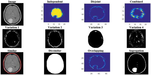
This subsection presents the experimental outputs using the “BraTS 2021 Task” [31] dataset and MATLAB software. To ensure experimental reproducibility, the BraTS 2021 dataset was partitioned into training, validation, and testing subsets following a fixed 70% / 15% / 15% split strategy. A controlled random seed (seed=42) was used during the data shuffle process to prevent bias from stochastic sample ordering. Prior to model training, all MRI volumes underwent standardized preprocessing, including NIfTI formatting verification, skull-stripping confirmation, and voxel-level intensity normalization using z-score scaling. All modalities (T1, T1Gd, T2, and FLAIR) were resized to a spatial resolution of 240×240 and harmonized to a unified anatomical template. During training, only non-affine augmentations were used to preserve tumor boundaries, including random flipping, small rotation (<10°), and contrast jittering. This configuration ensures consistency in feature space representation across the segmentation workflow and aligns with established reproducibility protocols in medical image computing. All BraTS mpMRI scans represent a) native (T1) and b) post-contrast T1-weighted (T1Gd), c) T2-weighted (T2), and d) T2 Fluid Attenuated Inversion Recovery (T2-FLAIR) volumes, and these were obtained under varying clinical parameters and using a variety of scanners at various data contributing centres. Manual annotation of all the imaging datasets has been done by one to four raters using the same annotation protocol, and their annotations accepted by the expert neuro-radiologists. Annotations include: GD-enhancing tumor (ET -label 4), peritumoral edematous/invaded tissue (ED -label 2), and necrotic tumor core (NCR -label 1), as defined in both the TMI paper of BraTS 2012-2013 and the most recent paper of BraTS summing up it. Their pre-processing, i.e. co-registering them to the same anatomical template, interpolating them to the same resolution (1 mm3) and skull-stripping them, yielded the ground truth data. The dataset provides three types of tumor inputs: native, weighted, and inverted which are classified using their detection. The number of training images is 6K+ and the testing images are 1.4K for assessment. The number of epochs used is 8 in this analysis for which the fully connected network is divided based on region-splitting conditions for mean and standard deviation. The learning network’s training rate is 0.6 to 1 targeting the above count of epochs. The epoch is continuously validated for a maximum of 10 regions such that the change in variation results in a start of new epoch. Therefore, the terminating condition is identified based on the classifications and variation values to ensure precise segment is identified. The experimental outputs are presented below using a sample input.
FCLN Error

Figure 6. Overall experimental outcomes
The given approach makes the uncertainty unanimous by means of an iterative procedure with the use of a Fully Connected Learning Network (FCLN). This network carries out two tasks at the same time, disjoint feature detection and uncertainty estimation. These operations are being done on similar and dissimilar regions and their outputs are pooled together so as to be trained simultaneously. The training process repeats itself till a common value of uncertainty is found. This is the event that, the two parallel processes (disjoint feature detection and uncertainty estimation) come up to a certain value of uncertainty. When this unanimous consensus is achieved, any further recurrence of the operations is suspended by the system, so that the most conservative measure of uncertainty has been considered. The steps of the process can be summarized in five steps and they include, first, the FCLN analyses the input information of the disjoint features and uncertainty. Second, same and different regions are processed at the same time. Third, the network keeps continue training and adjusting the weights depending on the results. Fourth, this process is repeated until both operations get the same value of uncertainty. Lastly, the training process is terminated when the unanimous uncertainty value is achieved. This method will ensure optimal performance where the measure of uncertainty is considered as being the most conservative (Refer to FCLN Error (Figure 6)).
In Table 3, the $\phi$ and $\nabla$ for different regions with their corresponding $\alpha_s$ and $\alpha_p$ values are presented.
The disjoint regions and the independent ones are classified at the classification phase. The unanimous value of uncertainty is identified using Eq. (10). The region extraction is done through the detection. The segregation is separated out of the segmentation process and presents improved region delineation. The splitting of regions is analyzed to result in the proper detection of region. The extraction of the features is implemented by the assignment of the weights of the number of neurons in ascertaining perceptron. The error pixel that is trained by the first layer is refined by the hidden layers and better region detection occurs. The overlapping is discussed to identify the brain tumors better according to this segmentation. The segmentation and the segregation is carried out in order to enhance the detection within brief time. The computation time of detection is reduced by separating the areas that are similar in features and not similar (Table 3).
Table 3. $\tau \phi$ and $\nabla$ for different conditions and regions
|
Conditions |
Regions |
$\mathbf{a}_0$ |
$\mathbf{g}^{\prime}$ |
$\omega_0, \omega^{\prime}(U)$ |
$\phi$ |
$\nabla$ |
|
$s_o \neq \tau$ |
2 |
0.8421 |
0.8967 |
0.9892 |
0.9852 |
±0.0201 |
|
4 |
0.8655 |
0.8645 |
0.9023 |
0.9132 |
±0.1055 |
|
|
6 |
0.8139 |
0.8561 |
0.9874 |
0.9134 |
±0.1171 |
|
|
8 |
0.9442 |
0.8327 |
0.9043 |
0.9084 |
±0.1079 |
|
|
10 |
0.9371 |
0.8822 |
0.9783 |
0.9515 |
±0.0922 |
|
|
$s_o=\tau$ |
2 |
0.8337 |
0.8010 |
0.9428 |
0.9027 |
±0.0963 |
|
4 |
0.8648 |
0.786 |
0.9707 |
0.9936 |
±0.0864 |
|
|
6 |
0.9297 |
0.7504 |
0.9853 |
0.9713 |
±0.0728 |
|
|
8 |
0.8597 |
0.7816 |
0.9422 |
0.992 |
±0.0811 |
|
|
10 |
0.8363 |
0.7226 |
0.9562 |
0.9948 |
±0.0702 |
|
|
$\tau$ Only |
2 |
0.8414 |
0.7138 |
0.9513 |
0.9819 |
±0.0492 |
|
4 |
0.8234 |
0.718 |
0.9744 |
0.952 |
±0.0299 |
|
|
6 |
0.8013 |
0.7712 |
0.9861 |
0.9251 |
±0.0318 |
|
|
8 |
0.8242 |
0.7858 |
0.9215 |
0.9206 |
±0.0413 |
|
|
10 |
0.8268 |
0.6246 |
0.9298 |
0.9352 |
±0.0309 |
The performance assessment is validated using the following metrics: precision, segmentation rate, uncertainty, detection time, and region detection. This assessment is performed as a comparative analysis by changing the number of regions (1 to 10) and feature extraction rates (0.1 to 1). The existing methods EDLF (Evidential Deep Learning Framework) [21], SCAU-Net (Self-Calibrated Attention U-Net) [25], and ASBTCNN (Automated Segmentation of Brain Tumor using CNN) [16] are paired with the proposed methods in this comparative performance assessment.
To ensure robustness, the proposed DSM-FCLN framework and baseline models were trained across five independent runs with varying initialization seeds (42, 77, 101, 128, and 256). All reported values are presented as mean ± standard deviation, and 95% confidence intervals were computed in accordance with model-to-model variation. This statistical reporting approach reflects stability across repeated trials rather than a single execution outcome. To further evaluate stability and sensitivity to initialization, the multi-run results were analyzed using variance-based sensitivity scoring. The proposed DSM-FCLN demonstrated low run-to-run fluctuation, with performance variation remaining within ±1.4% for segmentation rate and ±0.9% for precision. A paired t-test comparing the proposed model against the strongest baseline (SCAU-Net) confirmed that improvements were statistically significant (p<0.05). The narrow confidence intervals indicate that the observed performance gains are not incidental or seed-dependent but remain consistent across repeated training iterations. To ensure fair comparison, all baselines (EDLF, SCAU-Net, and ASBTCNN) were re-trained under identical experimental conditions. The same dataset split (70% training, 15% validation, 15% testing), preprocessing steps, and augmentation policies were applied consistently across all models. Training was standardized to 8 epochs, using the Adam optimizer with a learning rate of 0.001, batch size of 16, and controlled seed initialization (seed=42) to minimize stochastic variation. No model-specific tuning advantage was applied, and hyperparameter settings were aligned to prevent bias in model performance. This ensures that the reported improvements stem from methodological advantages rather than differences in training configuration as shown Table 4.
Table 4. Training configuration consistency across models
|
Parameter |
EDLF |
SCAU-Net |
ASBTCNN |
DSM-FCLN |
|
Train/Val/Test Split |
70/15/15 |
70/15/15 |
70/15/15 |
70/15/15 |
|
Epochs |
8 |
8 |
8 |
8 |
|
Optimizer |
Adam |
Adam |
Adam |
Adam |
|
Learning Rate |
0.001 |
0.001 |
0.001 |
0.001 |
|
Batch Size |
16 |
16 |
16 |
16 |
|
Augmentations |
Same |
Same |
Same |
Same |
|
Seed |
42 |
42 |
42 |
42 |
In Figure 7, the precision for the proposed work increases by identifying the similar and dissimilar regions. The feature extraction is performed based on the classification process that includes independent and disjoint. The precision is increased by determining the segmentation of images. The image segmentation is done by evaluating the pixels and decreasing the uncertainty and it is represented as $\sum_{\mathrm{a}_0}^{\mathrm{g}^{\prime}}\left[\phi * \mathrm{~m}_0\right]+\mathrm{l}_0-\tau$. In this number of pixels are detected from the respective regions. The region-based detection is done for the number of images and determining the disjoint. Thus, the proposed precision is improved in determining the segmentation. Eq. (3), states the uncertainty and decreases overlapping of pixels. The classification is carried out by splitting the independent and disjoint regions. The feature extraction is done from the MRI and the processing is done for the number of pixels and identifies the overlapping.


Figure 7. Precision analysis
The segmentation rate increases in Figure 8, by determining the uncertainty in the processing. Here, the similarities and dissimilar are identified to evaluate the segmentation process. The segmentation is evaluated by determining the classification of independent and disjoint regions and it is denoted as $\prod_{\mathrm{g}^{\prime}}^{\ln ^{\prime}}(\beta * \rho)+(\emptyset-\tau)$. In this computation step, the segregation is done from the segmentation method. Here, the processing is termed by splitting the region and evaluating the maximum disjoint identification. The analysis is done by assigning several neurons in connected layers. Here, $\left(\partial+\mathrm{m}_{\mathrm{n}} /_{\mathrm{g}^{\prime}}+\nabla\right)$ the splitting of regions along with the overlapping and non-overlapping pixels is examined. In this evaluation step, better segmentation is performed by using the FCNL. Thus, similar regions are segmented reducing the uncertainty in the proposed work. The segmentation of similar and dissimilar regions is done based on the classification process.


Figure 8. Segmentation rate analysis
In Figure 9, the uncertainty decreases by identifying the disjoint from the classification method. The maximum disjoint is identified by performing the segmentation method and it is represented as $\partial * \mathrm{e}^{\prime}+\mathrm{U} /(\rho+\tau)$. The computation is done for the detection of brain tumors in MRI. From this processing, the uncertainty is defined by extracting the necessary features from the input region. The desired features are extracted and split as independent and disjoint regions. Here, the uncertainty is defined by assigning the weights for the number of neurons in the connected network. The FCNL is proposed to decrease the uncertainty and detect the brain tumor by addressing the overlapping of pixels. The overlapping of pixels and uncertainty is estimated by equating Eq. (9). The processing is examined by improving the computation process by introducing the single hidden layer that is used to train similar and dissimilar regions.


Figure 9. Uncertainty analysis
The detection time decreases in Figure 10, by evaluating the better pixel identification from the MRI. The MRI extracts the necessary features and provides the classification method. The classification is done for the independent and disjoint regions and it is equated as $\mathrm{l}_{\mathrm{n}}+\left(\frac{\sum \mathrm{U} \nabla+\emptyset}{\mathrm{C} * \mathrm{~m}_0}\right)$. The computation for the proposed work shows the better detection of brain tumors by detecting overlapping pixels. Eq. (1) is used to derive the overlapping of pixels and eliminates the further processing step. The overlapping is examined for better identification of brain tumors based on this segmentation. The segmentation along with the segregation is done to improve the detection in less time. The computation time for detection decreases by splitting the regions which are similar in features and not similar. From this preliminary step, the processing step decreases and shows better detection. The detection time is reduced by identifying the disjoint region.


Figure 10. Detection time analysis
In Figure 11, the region detection is high in the proposed work by determining the uncertainty. The uncertainty value for the proposed work shows better results that are based on similar and dissimilar identification. The classification phase is used to distinguish the independent and disjoint regions. Eq. (10) is used to identify the unanimous uncertainty value. The detection is performed for the region extraction and it is represented as $\left[\left(\sum_{\mathrm{g}^{\prime}}^{\mathrm{l}_0} \omega_0+\omega^{\prime}\right)\right] * \mathrm{C}-\frac{\mathrm{m}_0}{\sigma+\mathrm{s}_0}$. The segregation is done from the segmentation process and shows better region detection and it is represented as $\beta(\rho+\tau) * \mathrm{~g}^{\prime}$.


Figure 11. Region detection analysis
The appropriate detection of region is analyzed from the splitting of regions. The feature extraction is done by assigning the weights for the number of neurons by determining perceptron. The hidden layers train the error pixel from the first layer and perform better region detection. Thus, the region detection is performed for better feature extraction. In the below Tables 5 and 6 below, the above study is summarized with the improvements of the proposed method compared to the existing methods.
Table 5. Comparative study summary for regions
|
Metrics |
EDLF |
SCAU-Net |
ASBTCNN |
DSM-FCLN |
|
Precision |
0.681 |
0.793 |
0.864 |
0.9211 |
|
Segmentation Rate |
0.826 |
0.867 |
0.913 |
0.9669 |
|
Uncertainty (/Region) |
0.189 |
0.141 |
0.105 |
0.0764 |
|
Detection Time (ms) |
611.11 |
435.31 |
337.88 |
105.997 |
|
Region Detection (%) |
67.21 |
73.49 |
84.1 |
94.715 |
Table 6. Comparative study summary for feature extraction rate
|
Metrics |
EDLF |
SCAU-Net |
ASBTCNN |
DSM-FCLN |
|
Precision |
0.692 |
0.797 |
0.861 |
0.9292 |
|
Segmentation Rate |
0.793 |
0.87 |
0.921 |
0.9652 |
|
Uncertainty (/Region) |
0.185 |
0.148 |
0.124 |
0.0867 |
|
Detection Time (ms) |
612.08 |
436.38 |
346.86 |
196.672 |
|
Region Detection (%) |
67.64 |
75.88 |
85.06 |
94.536 |
The proposed method achieves the following: 7.09% more precision, 9.82% more segmentation rate, 9.89% more region detection, 6.86% less uncertainty, and 12.84% less detection time.
The proposed method achieves the following: 7.29% more precision, 10.39% more segmentation rate, 9.17% more region detection, 6.56% less uncertainty, and 9.62% less detection time.
The proposed Disjoint Segmentation Method (DSM) with a Fully Connected Learning Network (FCLN) pays off with a number of clinically valuable gains in respect to brain tumor segmentation. The method will help improve the performance of the tumor boundary delineation by resolving the textural uncertain issues and pixel overlap, and thus the resulting treatment planning and tumor volume measurement might be more precise and be used to help improve the treatment planning process. The emphasis on minimizing uncertainties during the segmentation process might make clinicians have more accurate and consistent outcomes to make diagnoses and treatment decisions. The capacity of the approach to distinguish between similar and dissimilar areas, and detect disjoint features, may be especially helpful in the segmentation of tumors of heterogeneous nature or infiltrative ones. The process of segmentation would be more accurately automated, and thus the time and workload of manual segmentation by a radiologist would be decreased, resulting in more effective clinical processes. The DSM is compatible with most MRI modalities (T1, T1Gd, T2, T2-FLAIR) that are active in clinical practice to determine brain tumors. The proposed technique has been demonstrated to have better precision, higher rate of segmentation, region detection and less uncertainty and detection time than current techniques. The above enhancements may be in the form of more robust clinical evaluations and possibly incorporated into wider clinical decision support systems that would assist in the planning and monitoring of treatment.
This article introduced and briefed on the functions of the disjoint segmentation method for uncertainty reduction in detecting brain tumors using MR images. This proposed method extracts standard deviation and mean features for the inputs and classifies them as independent and disjoint. These classifications are used by the fully connected network for identifying uncertainty across similar and dissimilar regions. This process is recurrent over the disjoint and similar regions concurrently regardless of the disjoint regions. The maximum disjoint regions are identified using recurrent training between overlapping and pixel-varying regions. Therefore, the precision is improved using two simultaneous operations: feature detection and uncertainty computation. This is suppressed using multiple concurrent training until the least possible uncertainty value is reached. In this case, if both the concurrent process identifies the uncertainty value as unanimous then, the recurrency is halted. The non-overlapping regions are segregated from the maximum disjoint regions in the segmentation process. Therefore, the proposed method achieves the following: 7.09% more precision, 9.82% more segmentation rate, 9.89% more region detection, 6.86% less uncertainty, and 12.84% less detection time. This proposed method though reduces the uncertainties in MRI segmentation; the finest portion analysis requires multiple varying regions. This reduces the actual precision demand regardless of the peak improvement for which a pre-classified segment-based analysis is required. Thus, the segmentation process relies on unidentified features over the parted regions for retaining precision. Although the proposed method demonstrates strong improvements in uncertainty reduction and segmentation accuracy, future extensions will incorporate explainability mechanisms such as activation-based visualizations and interpretability maps to better analyze feature importance and enhance clinical trust in the model outputs.
[1] Rajput, S., Kapdi, R., Roy, M., Raval, M.S. (2024). A triplanar ensemble model for brain tumor segmentation with volumetric multiparametric magnetic resonance images. Healthcare Analytics, 5: 100307. https://doi.org/10.1016/j.health.2024.100307
[2] Peng, Y., Sun, J. (2023). The multimodal MRI brain tumor segmentation based on AD-Net. Biomedical Signal Processing and Control, 80: 104336. https://doi.org/10.1016/j.bspc.2022.104336
[3] Abidin, Z.U., Naqvi, R.A., Haider, A., Kim, H.S., Jeong, D., Lee, S.W. (2024). Recent deep learning-based brain tumor segmentation models using multi-modality magnetic resonance imaging: A prospective survey. Frontiers in Bioengineering and Biotechnology, 12: 1392807. https://doi.org/10.3389/fbioe.2024.1392807
[4] Zhang, D., Wang, C., Chen, T., Chen, W., Shen, Y. (2024). Scalable swin transformer network for brain tumor segmentation from incomplete MRI modalities. Artificial Intelligence in Medicine, 149: 102788. https://doi.org/10.1016/j.artmed.2024.102788
[5] Farhan, A.S., Khalid, M., Manzoor, U. (2025). XAI-MRI: an ensemble dual-modality approach for 3D brain tumor segmentation using magnetic resonance imaging. Frontiers in Artificial Intelligence, 8: 1525240. https://doi.org/10.3389/frai.2025.1525240
[6] Xu, C., Yang, Y., Xia, Z., Wang, B., Zhang, D., Zhang, Y., Zhao, S. (2023). Dual uncertainty-guided mixing consistency for semi-supervised 3D medical image segmentation. IEEE Transactions on Big Data, 9(4): 1156-1170. https://doi.org/10.1109/TBDATA.2023.3258643
[7] Zhou, T., Zhu, S. (2023). Uncertainty quantification and attention-aware fusion guided multi-modal MR brain tumor segmentation. Computers in Biology and Medicine, 163: 107142. https://doi.org/10.1016/j.compbiomed.2023.107142
[8] Shi, Y., Zu, C., Yang, P., Tan, S., Ren, H., Wu, X., Zhou, J., Wang, Y. (2023). Uncertainty-weighted and relation-driven consistency training for semi-supervised head-and-neck tumor segmentation. Knowledge-Based Systems, 272: 110598. https://doi.org/10.1016/j.knosys.2023.110598
[9] Chen, Z., Peng, C., Guo, W., Xie, L., Wang, S., Zhuge, Q., Wen, C., Feng, Y. (2023). Uncertainty-guided transformer for brain tumor segmentation. Medical & Biological Engineering & Computing, 61(12): 3289-3301. https://doi.org/10.1007/s11517-023-02899-8
[10] Li, W., Huang, W., Zheng, Y. (2024). CorrDiff: Corrective diffusion model for accurate MRI brain tumor segmentation. IEEE Journal of Biomedical and Health Informatics, 28(3): 1587-1598. https://doi.org/10.1109/JBHI.2024.3353272
[11] Yadav, A.C., Kolekar, M.H., Zope, M.K. (2025). Modified recurrent residual attention U-Net model for MRI-based brain tumor segmentation. Biomedical Signal Processing and Control, 102: 107220. https://doi.org/10.1016/j.bspc.2024.107220
[12] Pedada, K.R., Rao, B., Patro, K.K., Allam, J.P., Jamjoom, M.M., Samee, N.A. (2023). A novel approach for brain tumour detection using deep learning based technique. Biomedical Signal Processing and Control, 82: 104549. https://doi.org/10.1016/j.bspc.2022.104549
[13] Nassar, S.E., Elnakib, A., Abdallah, A.S., El-Azim, M.A. (2024). Toward enhanced brain tumor segmentation in MRI: An ensemble deep learning approach. In 2024 IEEE Canadian Conference on Electrical and Computer Engineering (CCECE), Kingston, Canada, pp. 483-488. https://doi.org/10.1109/CCECE59415.2024.10667250
[14] Liu, Z., Tong, L., Chen, L., Jiang, Z., Zhou, F., Zhang, Q., Zhang, X., Jin, Y., Zhou, H. (2023). Deep learning based brain tumor segmentation: A survey. Complex & Intelligent Systems, 9(1): 1001-1026. https://doi.org/10.1007/s40747-022-00815-5
[15] Ullah, M.S., Khan, M.A., Albarakati, H.M., Damaševičius, R., Alsenan, S. (2024). Multimodal brain tumor segmentation and classification from MRI scans based on optimized DeepLabV3+ and interpreted networks information fusion empowered with explainable AI. Computers in Biology and Medicine, 182: 109183. https://doi.org/10.1016/j.compbiomed.2024.109183
[16] Rajendran, S., Rajagopal, S.K., Thanarajan, T., Shankar, K., Kumar, S., Alsubaie, N.M., Ishak, M.K., Mostafa, S.M. (2023). Automated segmentation of brain tumor MRI images using deep learning. IEEE Access, 11: 64758-64768. https://doi.org/10.1109/ACCESS.2023.3288017
[17] Tejashwini, P.S., Thriveni, J., Venugopal, K.R. (2025). A novel SLCA-UNet architecture for automatic MRI brain tumor segmentation. Biomedical Signal Processing and Control, 100: 107047. https://doi.org/10.1016/j.bspc.2024.107047
[18] Hernandez-Gutierrez, F.D., Avina-Bravo, E.G., Zambrano-Gutierrez, D.F., Almanza-Conejo, O., Ibarra-Manzano, M. A., Ruiz-Pinales, J., Ovalle-Magallanes, E., Avina-Cervantes, J.G. (2024). Brain tumor segmentation from optimal MRI slices using a lightweight U-Net. Technologies, 12(10): 183. https://doi.org/10.3390/technologies12100183
[19] Rabby, S.F., Arafat, M.A., Hasan, T. (2024). BT-Net: An end-to-end multi-task architecture for brain tumor classification, segmentation, and localization from MRI images. Array, 22: 100346. https://doi.org/10.1016/j.array.2024.100346
[20] Qin, J., Xu, D., Zhang, H., Xiong, Z., Yuan, Y., He, K. (2025). BTSegDiff: Brain tumor segmentation based on multimodal MRI dynamically guided diffusion probability model. Computers in Biology and Medicine, 186: 109694. https://doi.org/10.1016/j.compbiomed.2025.109694
[21] Li, H., Nan, Y., Del Ser, J., Yang, G. (2023). Region-based evidential deep learning to quantify uncertainty and improve robustness of brain tumor segmentation. Neural Computing and Applications, 35(30): 22071-22085. https://doi.org/10.1007/s00521-022-08016-4
[22] Alwadee, E.J., Sun, X., Qin, Y., Langbein, F.C. (2025). LATUP-Net: A lightweight 3D attention U-Net with parallel convolutions for brain tumor segmentation. Computers in Biology and Medicine, 184: 109353. https://doi.org/10.1016/j.compbiomed.2024.109353
[23] Sun, J., Hu, M., Wu, X., Tang, C., Lahza, H., Wang, S., Zhang, Y. (2024). MVSI-Net: Multi-view attention and multi-scale feature interaction for brain tumor segmentation. Biomedical Signal Processing and Control, 95: 106484. https://doi.org/10.1016/j.bspc.2024.106484
[24] Chen, Y., Tang, T., Kim, T., Shu, H. (2025). UKAN-EP: Enhancing U-KAN with efficient attention and pyramid aggregation for 3D multi-modal MRI brain tumor segmentation. BMC Medical Imaging. arXiv E-Prints, arXiv-2408. https://doi.org/10.1186/s12880-025-02053-w
[25] Liu, D., Sheng, N., Han, Y., Hou, Y., Liu, B., Zhang, J., Zhang, Q. (2023). SCAU-net: 3D self-calibrated attention U-Net for brain tumor segmentation. Neural Computing and Applications, 35(33): 23973-23985. https://doi.org/10.1007/s00521-023-08872-8
[26] Mostafa, A.M., El-Meligy, M.A., Alkhayyal, M.A., Alnuaim, A., Sharaf, M. (2023). A framework for brain tumor detection based on segmentation and features fusion using MRI images. Brain Research, 1806: 148300. https://doi.org/10.1016/j.brainres.2023.148300
[27] Zhang, G., Zhou, J., He, G., Zhu, H. (2023). Deep fusion of multi-modal features for brain tumor image segmentation. Heliyon, 9(8): e19266. https://doi.org/10.1016/j.heliyon.2023.e19266
[28] Qureshi, S.A., Chaudhary, Q.U.A., Schirhagl, R., Hussain, L., Aman, H., Duong, T.Q., Nawaz, H., Ren, T., Galenchik-Chan, A. (2024). RobU-Net: A heuristic robust multi-class brain tumor segmentation approaches for MRI scans. Waves in Random and Complex Media, 1-51. https://doi.org/10.1080/17455030.2024.2366837
[29] Rutoh, E.K., Guang, Q.Z., Bahadar, N., Raza, R., Hanif, M.S. (2024). GAIR-U-Net: 3D guided attention inception residual u-net for brain tumor segmentation using multimodal MRI images. Journal of King Saud University-Computer and Information Sciences, 36(6): 102086. https://doi.org/10.1016/j.jksuci.2024.102086
[30] Liu, J., Bhatti, U. A., Zhang, J., Zhang, Y., Huang, M. (2025). Ef-VPT-net: Enhanced feature-based vision patch transformer network for accurate brain tumor segmentation in magnetic resonance imaging. IEEE Journal of Biomedical and Health Informatics, 1-14. https://doi.org/10.1109/JBHI.2025.3526976
[31] BRaTS 2021 Task 1 Dataset. https://www.kaggle.com/datasets/dschettler8845/brats-2021-task1.