Kavery Verma![]() | Subodh Srivastava
| Subodh Srivastava![]() | Ritesh Kumar Mishra*
| Ritesh Kumar Mishra*![]()
© 2025 The authors. This article is published by IIETA and is licensed under the CC BY 4.0 license (http://creativecommons.org/licenses/by/4.0/).
OPEN ACCESS
Magnetic Resonance (MR) imaging is a powerful digital imaging technique that provides detailed insights into the abnormal structure and function of the brain. However, during image acquisition, these MR images are affected by artifacts and noise, which primarily follow the Rician distribution. The quality of the image is diminished by these inconsistencies, limiting the interpretive effectiveness of radiologists. To overcome these issues, an optimized reformed Anisotropic Diffusion Unsharp Masking (OADUM) filter has been proposed that preserves the sharpness, contrast, edges, and fine details of Rician noise-corrupted MR images. In this proposed methodology, the edge threshold constant of the diffusion coefficient is automated using the Enhancement Measurement on Entropy (EMEE) method and clubbed with Maximum Likelihood Estimation (MLE) instead of manual calculation. Further, to improve the quality of smoothen images, the Greedy Search Optimization (GSO) algorithm is applied, where Peak Signal-to-Noise Ratio (PSNR) is taken as a fitness function. The performance of the restored and enhanced output image has been analyzed with earlier existing methods in both qualitative and quantitative ways on COBRE dataset. The quantitative assessment parameters taken are MSE, PSNR, UQI, SSIM, MS-SSIM, NAE, CP, and DE, whose average values are coming out to be 0.4486, 51.9872, 0.8268, 0.9947, 0.9857, 0.6075, 0.9862, and 5.0547, respectively. Experimental results demonstrated that the proposed methodology outperformed earlier existing state-of-the-art methods, significantly improving the visual quality and performance indexes of the dataset, thereby making the method more useful for diagnostic and clinical purposes.
denoising, enhancement, Magnetic Resonance (MR) imaging, optimization, Rician noise
Magnetic Resonance imaging has revolutionized medical diagnosis by providing unparalleled anatomical details and functional information about the brain. Precise detection of abnormalities within the brain tissue is crucial for accurate diagnosis and timely intervention. However, Magnetic Resonance (MR) images are inherently susceptible to noise [1]. Due to the thermal turbulence of electrons, MR images are sensitive mostly to Rician noise [2]. The presence of Rician noise in MR images can significantly degrade image quality, particularly at low Signal-to-Noise Ratio (SNR) [3]. This noise can obscure critical features, hindering the accurate diagnosis of abnormalities [4]. Furthermore, existing denoising methods often fail to balance noise reduction and preservation of structural detail, leading to dusky images and misdiagnosis of diseases. According to a survey by the National Center for Biotechnology Information in 2024, the misdiagnosis rate of Schizophrenia (SZ) in clinical practice can be as high as 25% [5]. Approximately 30% of individuals with SZ demonstrate treatment-resistant traits and respond inadequately to conventional antipsychotic medications, which presents a significant challenge [6]. Further, a report from the Miami Neuroscience Centre indicates that 80,000 new cases of brain cancer arise in the US each year [7]. This paper proposes a novel method to address these challenges and improve the quality of Rician noise-corrupted MR images. The proposed methodology integrates two powerful techniques, reformed Anisotropic Diffusion Unsharp Masking (ADUM) with Greedy Search Optimization (GSO) algorithm with the Peak Signal-to-Noise Ratio (PSNR) serving as the fitness function. This method effectively reduces noise while preserving crucial features such as edges and contours. It ensures that fine details remain visible, even in regions characterized by low contrast or noise, thereby enhancing image quality. The method begins with the removal of noise to improve the quality of image. Here modified Anisotropic Diffusion (AD) acts as a sophisticated denoising filter [8]. To reduce the Rician noise, AD filter is integrated with Maximum Likelihood Estimation (MLE) simultaneously automating the edge threshold constant of diffusion coefficient by Enhancement Measurement on Entropy (EMEE) method [9]. Unlike traditional filters that blur the entire image, this reformed AD selectively smooths out the noise while preserving sharp edges and crucial structural details within the brain tissue [10, 11]. Here, the regularization parameter for the smoothed image is varied by the average SNR calculation. Following denoising, optimization of these images is done with the computation of the Global Variance (GV), using GSO algorithm, which informs the subsequent processing steps where Peak Signal-to-Noise Ratio (PSNR) is taken as fitness function [12]. Unlike fixed-parameter approaches, this algorithm actively searches for the best possible configuration [13]. This technique sharpens edges by highlighting the difference between neighboring pixels [14]. Through a series of iterative adjustments guided by the greedy search, the method achieves optimal results in terms of noise reduction and overall image clarity. After that, scaling of the edge image is done using manual and random search optimization followed by employing modified Unsharp Masking (UM) to enhance the contrast and sharpness of image [15]. Finally, the restored and enhanced output image obtained from modified UM improves the visibility of subtle anatomical features within the brain, making it visually clear and allows for accurate diagnosis.
The effectiveness of the proposed method is thoroughly assessed by conducting both qualitative and quantitative comparisons with existing state-of-the-art techniques. The experimental results demonstrate that the proposed method significantly improves the visual quality of Rician noise-corrupted MR images. The enhanced clarity and detail afforded by this method hold substantial promise for diagnostic and clinical applications, potentially leading to more accurate and reliable medical assessments.
1.1 Motivation
Brain diseases are constantly increasing due to stressful lifestyles, environmental factors, and chronic diseases. For accurate diagnoses of these diseases, an enhanced quality of MR image is required. Despite their high-resolution device imaging capabilities, MR images are frequently subjected to noise primarily Rician noise, which can obscure crucial anatomical details and hinder accurate clinical assessments. To address this issue, the proposed methodology aims to achieve superior image detail and clarity by systematically exploring parameter space. This advancement promises to improve diagnostic accuracy and patient outcomes, providing a robust solution to the persistent challenge of Rician noise in MR imaging.
1.2 Key contributions and organization
The fundamental contributions of this paper are as follows:
(1) Identification of noise.
(2) Develop a novel method combining reformed anisotropic diffusion unsharp masking filter and a greedy search optimization algorithm to restore and enhance MR images corrupted by Rician noise while preserving the important structural details.
(3) Systematically explored the parameter space to ensure an optimal balance between noise reduction and detail enhancement.
(4) Significantly improved the visual clarity and diagnostic utility of MR images.
(5) Addressed a critical challenge in medical imaging with a robust and practical solution to Rician noise.
The rest of this manuscript is organized as follows: Section 2. gives details about previous works done in this area. Section 3. discusses about the dataset taken, and describes the experimental setup of the proposed methodology and the different performance assessment parameters taken. Results are drawn and discussed in Section 4. Finally, a conclusion and future scope of this methodology is discussed in Section 5.
This section gives details about some earlier work done on denoising, enhancement, and optimization. Hu et al. introduced Non-Local Means (NLM) filter using random sampling (SNLM) method which reduces noise, improves computational quality, and competitive denoising results [16]. Nguyen et al. enhanced the classical NLM filter by introducing improved Non-Local Self-Weight (NLSW) estimation techniques [17]. While the method improves denoising performance, it has higher computational complexity and can be time consuming, especially for large image data. Chang et al. introduces Trilateral Filter (TLF) with extended the Bilateral Filter (BF) by adding an extra intensity similarity function and an adaptive entropy function to improve noise reduction [18]. While the self-regulating TLF demonstrates significant advancements and effectiveness in denoising brain MR images, it faces limitations related to automation challenges and potential over-smoothing. Zhang et al. proposed denoising method, MR image utilizes a combination of image Low-Rank and Sparse Gradient prior Gaussian Mixture (LRSGM) model clustering and iterative optimization techniques to achieve effective noise reduction while preserving image details [19]. The use of Gaussian Mixture (GM) for clustering and the iterative algorithm can be computationally intensive, requiring significant processing power and time, which might be a limitation for real-time applications or large datasets. The proposed method of Kanoun et al. enhances the traditional NLM filter by incorporating the Kolmogorov-Smirnov (KS) distance for better patch similarity estimation [20]. This method coupled with local anisotropy analysis (AKSNLM), results in the denoising and preservation of image details. While the method is effective at moderate noise levels, its performance may degrade in extremely noisy conditions. The anisotropic weighting and KS distance calculation might not be sufficient to handle very high noise levels, leading to the potential loss of important image details. Rai et al. proposed Augmented Deep Residue Network (ADRN) framework which performs denoising by combining the strengths of both Residual Learning (RL) and Dictionary Learning (DCL) [21]. The performance of the denoising framework is highly dependent on the quality and diversity of the training data. Also, the integration of RL and DCL in a single framework adds complexity to the implementation. Hou et al. utilizes truncated residual based plug-and-play Alternating Direction Method of Multipliers (ADMM) framework called TRPA, which enables the incorporation of pre-trained denoisers to address the denoising subproblem in ADMM-based MR image reconstruction [22]. TRPA relies on the effectiveness of pre-trained denoisers. If the denoiser is not well-optimized for the specific noise characteristics or MR images being reconstructed, the overall performance of TRPA may be compromised. Chuang et al. proposed a denoising method which is Score-based Reverse Diffusion Sampling (SRDS), to tackle the challenges of noise in MR image scans, offering robust performance on diverse and complex noise distributions [23]. It enhances image resolution, and quantifies uncertainty with significant improvements over Traditional Minimum Mean Squared Error (MMSE) based methods. The sampling approach may involve complex computations and a sophisticated architecture, resulting in high computational demands. This complexity might limit its practicality in real time applications. The scalability of the model to larger datasets or different MR imaging devices is yet to be extensively tested. Variations in imaging hardware and acquisition parameters could impact the performance of the model. Huang et al. had proposed a method that integrates a self-supervised denoising network with a plug-and-play optimization framework [24]. Here, the concept of Regularization by Denoising (RED) is used to enhance MR image reconstruction. This approach named DURED imposes a denoising network to act as a regularizer, ensuring high-quality reconstruction by incorporating imaging physics. However, this approach is dependent on the quality of the denoising network, which may lead to longer processing time, computational complexity, integration challenges with clinical workflows, and risk of overfitting for small MR image data. Addressing these limitations is essential for improving the robustness, efficiency, and applicability of the proposed denoising methods across diverse imaging contexts. Table 1 summarizes these earlier methods on denoising and enhancement.
Table 1. Earlier reported works on denoising and enhancement
|
Author |
Year |
Method |
Remark |
|
Hu et al. [16] |
2016 |
SNLM |
Requires accurate selection of the sampling ratio. |
|
Nguyen et al. [17] |
2017 |
NLSW |
Higher computational complexity and time consumption. |
|
Chang et al. [18] |
2018 |
TLF |
Automation challenges and potential over-smoothing. |
|
Zhang et al. [19] |
2019 |
LRSGM |
Significant processing power and time. |
|
Kanoun et al. [20] |
2020 |
AKSNLM |
Effective at moderate noise levels. |
|
Rai et al. [21] |
2021 |
ADRN |
Dependence on high-quality training data and computational complexity. |
|
Hou et al. [22] |
2022 |
TRPA |
Dependence on pre-trained denoisers. |
|
Chung et al. [23] |
2023 |
SRDS |
High computational demand and scalability issues. |
|
Huang et al. [24] |
2024 |
DURED |
Longer processing time and the risk of overfitting. |
This section offers a comprehensive overview of the proposed methodology and the dataset employed for this analysis.
3.1 Datasets
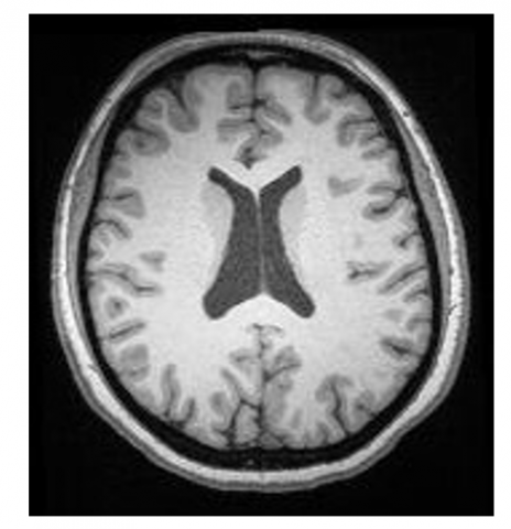
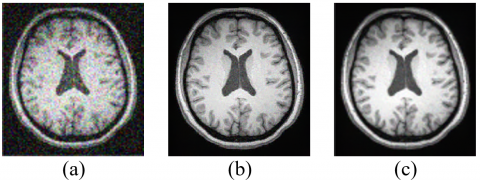
The dataset for this study was provided by the Center for Biomedical Research Excellence (COBRE) [25]. It includes raw anatomical and functional magnetic resonance imaging brain data from 72 patients diagnosed with schizophrenia and 75 healthy control subjects. The dataset consists of sample MR image of patients with age ranges from 18 to 65 years. Class imbalance does not affect the performance of the proposed method, as it operates independently for each individual image. Figure 1 shows sample MR image view of a patient suffering from Schizophrenia. Sample images contain three different orientation Axial, Coronal, and Sagittal scan of brain MR image.
(a)
(b)
(c)
Figure 1. Sample MR image view of a Schizophrenia patient, (a) Axial, (b) Coronal, and (c) Sagittal from COBRE dataset [25]
3.2 Methodology
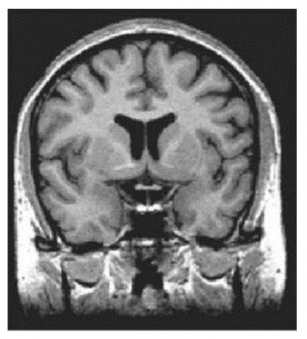
The block diagram of methodology taken for implementation of the proposed methods are shown in Figure 2. First and foremost, identification of noise in MR images is done. In order to have noise – free MR images, the proposed method starts with denoising using reformed AD filter followed by optimization and modified UM to obtain a restored and enhanced output image. The detail description of proposed methodology is explained below in mathematical way.
3.2.1 Proposed methodology with mathematical evaluation
With pixel-by-pixel magnitude calculation of real and imaginary section of MR image, the noise distribution identified is Rician as both the section is distorted by uncorrelated Gaussian noise with zero-mean ($\mu$=0) equal variance $\sigma^2$ [26]. Noisy corrupted image ‘$I_\eta$’ is given as:
$I_\eta=\sqrt{I_R^2+I_I^2}$ (1)
where, ‘$I_R$’ denotes real part of noisy image and ‘$I_I$’ is the imaginary part of noisy image.
The Rician Probability Density Function (PDF) of noisy MR image of pixel intensity ‘$M$’ is given as [27]:
$p(I / M)=\frac{M}{\sigma^2} e^{\left(-\frac{\left(M^2+I^2\right)}{2 \sigma^2}\right)} J_0\left(\frac{I M}{\sigma^2}\right) H(M)$ (2)
where, ‘I’ denotes the noise-free image, ‘$\sigma^2$’ is the Rician noise variance, ‘$J_0(.)$’ is zero-order modified Bessel’s function, and ‘$H(.)$’ represents the Heaviside function.
For MR image ‘$M$’, the magnitude of a signal cannot be negative. So, the value of $H(M)$=1, then, the Rician PDF is given as [28]:
$p(I / M)=\frac{M}{\sigma^2} e^{\left(-\frac{\left(M^2+I^2\right)}{2 \sigma^2}\right)} J_0\left(\frac{I M}{\sigma^2}\right)$ (3)
Here, noisy image ‘$M$’ is processed using an Anisotropic Diffusion (AD) filter, where the diffusion is governed by the MLE and EMEE for the noise-free image ‘$I$’. This filter aims to reduce noise while preserving essential structural details and edges in the image.
For ‘$n$’ set of observations, the likelihood function is given as [29]:
$L(p(I / M))=\sum_{i=1}^n \ln \left(\frac{M}{\sigma^2} e^{\left(-\frac{\left(M^2+I^2\right)}{2 \sigma^2}\right)} J_0\left(\frac{I M}{\sigma^2}\right)\right)$ (4)
Figure 2. Framework for proposed methodology to obtain denoised and enhanced MR image
For maximum likelihood estimation [30]:
$\frac{\partial}{\partial I} L(p(I / M))=0$ (5)
The general regularization function of the Anisotropic Diffusion equation is [31]:
$f(I)=\nabla .(c(| | \nabla I| |) \nabla I$ (6)
where, ‘$c(\|\nabla I\|)$’ is the diffusion coefficient whose value is given as:
$c(\|\nabla {I}\|)=\frac{1}{1+\left(\frac{\nabla {I}}{\beta}\right)^2}$ (7)
where, ‘$\beta$’ is a constraint of the diffusion coefficient.
Here, the value of ‘$\beta$’ is calculated as edge threshold value of Enhancement Measurement based on Entropy (EMEE). EMEE focusses on maximising local entropy around edges, in contrast to traditional methods that depend on global intensity distributions [32, 33]. It enhances edge regions adaptively, maintaining fine details even in areas with low contrast or noise [34, 35]. By directly linking entropy to edge strength, EMEE ensures superior edge preservation compared to conventional entropy-based techniques [36, 37].
The reformed diffusion coefficient is given as [38]:
$c^{\prime}(\|\nabla {I}\|)=\frac{1}{1+\left(\frac{\nabla {I}}{\beta^{\prime}}\right)^2}$ (8)
where, ‘$\beta^{\prime}$'’ is a threshold value of EMEE that controls the sensitivity to edges. The value is given as [39]:
$\beta^{\prime}=\frac{1}{p_1 p_2} \sum_{m=1}^{p_1} \sum_{l=1}^{p_2} \alpha\left(\frac{I_{\max }^{l, m}}{I_{\min }^{l, m}}\right)^\alpha \frac{I_{\max }^{l, m}}{I_{\min }^{l, m}}$ (9)
where, ‘$p_1$’ and ‘$p_2$’ show the number of cells used to split the denoised image, ‘$I_{\max }^{l, m}$’ denotes maximum values of pixel in each block of denoised image, ‘$I_{\min }^{l, m}$’ denotes minimum values of pixel in each block of denoised image, and ‘$\alpha$’ is the scaling factor.
The Energy functional of image ‘$I$’ that is ‘$E(I)$’ obtained from a reformed AD filtered image is given as [40]:
$E(I)=\arg _\min\left[\int_{\Omega}\left[\frac{\partial}{\partial I} L(p(I / M))+\gamma f(I)\right] d \Omega\right]$ (10)
where, ‘$\gamma$’ is called the regularization parameter, whose value is given as [41]:
$\gamma=\frac{1}{A v g . S N R}$ (11)
where, ‘$SNR$’ denotes signal to noise ratio.
The value of ‘$Avg.SNR$’ is given as:
$Avg.S N R=\frac{\text { mean }}{ { standard\ deviation }}=\frac{\mu}{\sigma}$ (12)
The denoised filtered output image obtained is represented as:
$\frac{\partial E(I)}{\partial t}=-\frac{1}{\sigma^2}+\frac{2 k_1}{I}+\gamma \nabla .\left(c^{\prime}(| | \nabla I| |) \nabla I\right)$ (13)
Further, the discretization of the above Eq. (13) is given as:
$\frac{I^{n+1}(i, j)-I^n(i, j)}{\Delta t^n}=\frac{I^n(i, j)}{\sigma^2}+\frac{2 k_1}{I}+\gamma \nabla .\left(c^{\prime}(\|\nabla I\|) \nabla I\right)$ (14)
Again, it can be written as:
$I^{n+1}(i, j)=I^n(i, j)+\Delta t\left[\frac{I^n(i, j)}{\sigma^2}+\frac{2 k_1}{I}+\gamma \nabla .\left(c^{\prime}(| | \nabla I \mid) \nabla I\right)\right]$ (15)
where, ‘ $i$ ’ and ‘ $j$ ’ are the pixel indices of an image ‘ $I$ ’, ‘ $\Delta t$ ’ is the grid constant, and ‘ $n$ ’ is the number of iterations.
Finally, the value of the filtered image can be given as:
$\begin{gathered}I^{\prime}=I^n(i, j)+\Delta t\left[ \frac{I^n(i, j)}{\sigma^2} + \frac{2k_1}{I} + \gamma \nabla.\left( c^{\prime}(\|\nabla I\|) \nabla I \right) \right]\end{gathered}$ (16)
To incorporate the global variance (GV) into the reformed anisotropic filtered image '$I^{\prime}$' for Greedy Search Optimization (GSO), the global variance '$\sigma_g^2$' of the filtered MR image '$I^{\prime}$' is calculated as [42]:
$\sigma_g^2=\frac{1}{P \times N} \sum_{i=1}^P \sum_{j=1}^N\left(I_{i j}^{\prime}-\mu\right)^2$ (17)
where, '$P$' and '$N$' are the dimensions of the image, '$I_{i j}^{\prime}$' is the intensity of the pixel at position ($i,j$), and '$\mu$' is the mean intensity of the image.
The value of '$\mu$' the mean intensity of the image is given as:
$\mu=\frac{1}{P \times N} \sum_{i=1}^P \sum_{j=1}^N I_{i j}^{\prime}$ (18)
Now, adding the GV '$\sigma_g^2$', to the output of the filtered image '$I$', the value of the reformed output image obtained is given as:
$I^r=I^{\prime}+\sigma_g^2$ (19)
GSO aims to define an objective function and iteratively make local adjustments to enhance the reformed image ‘$I^r$’ obtained from the previous step. The stopping condition for the GSO algorithm determines the condition where the optimization function should terminate the number of iterations [43]. In the proposed methodology, PSNR is taken as fitness function for the GSO. Convergence threshold and max. number of iterations clearly define stopping condition for GSO algorithm. Mathematically it can be defined as:
Suppose ‘$n$’ be define as number of iteration and ‘$\varepsilon$’ denotes convergence threshold, then stopping condition for GSO algorithm can be defined as [44]:
$\left|P S N R_n-P S N R_{n-1}\right|<\varepsilon$ (20)
where, value of ‘$\varepsilon$’ is a positive number such as around 0.001 dB or 0.01 dB.
This shows that there is no further scope for improvement in PSNR, so the optimization algorithm stops. The proposed method achieves the maximum PSNR value of 51.9872 dB for $n$ = 50, the number of iterations.
Let '$J$' denote the optimized output image after performing GSO on '$I^r$'. The objective function '$E(J)$' can be defined as:
$\begin{gathered}E(J) = \sum_{i, j} \left[ \left(I_{i j}^r - J_{i j}\right)^2 + \lambda \sum_{\left(i', j'\right) \in \mathcal{N}(i, j)} \left(J_{i j} - J_{i' j'}\right)^2 \right]\end{gathered}$ (21)
where, '$\lambda$' is a regularization parameter that balances fidelity to the original noisy image and smoothness, and '$\mathcal{N}(i, j)$' denotes the set of neighbouring pixels of $(i,j)$.
This objective function has two components that is data fidelity term '$\left(I_{i j}^r-J_{i j}\right)^2$' which shows the output image '$J$' remains close to the original noisy image '$I^r$' and the smoothness term '$\left(J_{i j}-J_{i^{\prime} j^{\prime}}\right)^2$', which shows the output image '$J$' to smoothed by the fine differences between neighboring pixels.
The GSO algorithm evaluates the objective function '$E(J)$' locally and updates the pixel value '$J_{i j}$' to minimize the local objective function.
Mathematically, it can be written as:
$J_{i j}{ }^{(k+1)}=J_{i j}{ }^{(k)}+\Delta J_{i j}$ (22)
where, '$\Delta J_{i j}$' is the change that minimizes the local objective function '$E$' at pixel ($i,j$).
The iterative process is done until the objective function '$E(J)$' converges or until a maximum number of iterations is reached.
Hence, the smoothen output image obtained after the GSO algorithm can be expressed as:
$J^{\prime}={argmin} \sum_{i, j}\left(\left(I_{i j}^r-J_{i j}\right)^2+\lambda \sum_{\left(i^{\prime}, j^{\prime}\right) \in \mathcal{N}(i, j)}\left(J_{i j}-J_{i^{\prime} j^{\prime}}\right)^2\right)$ (23)
where, '$J^{\prime}$' represents the optimized image or smoothen image obtained after filtering Rician noise using reformed AD, adding global variance, and refining with greedy search optimization. The optimization ensures that the image is smooth and retains essential features while minimizing noise.
Further, edge images can be calculated as follows:
$I_{E d g e}=M-J^{\prime}$ (24)
Again, the modified unsharp masked image is given as:
$I_{U M}=\alpha I_{E d g e}$ (25)
where, '$\alpha$' is a weighted parameter known as the scaling factor $(\alpha>0)$ that determines the level of sharpness. The value of '$\alpha$' is calculate with the help of random search optimization.
This formula encapsulates the entire process, combining the benefits of noise reduction, edge enhancement, and the addition of the original image details.
Algorithm 1 depicts the pseudocode for the proposed methodology. Also, the preferred values of parameters taken for this methodology are given in Table 2.
Table 2. Detail description of parameters taken for proposed methodology
|
Parameters |
Description |
Value |
|
$\Delta t$ |
Grid constant |
0.1 |
|
$n$ |
Number of iterations |
50 |
|
$\beta^{\prime}$ |
Threshold value for reformed AD |
10 to 50 |
|
$\gamma$ |
Regularization parameter |
Eq. (11) |
|
$\sigma_g^2$ |
Global variance |
Eq. (17) |
|
$\mu$ |
Mean intensity |
Eq. (18) |
|
$\lambda$ |
Diffusion parameter |
0 to 1.0 |
|
$\alpha$ |
Weighted parameter |
$\alpha$ > 0 |
|
Algorithm 1: Pseudo code for proposed method |
|
Input: Read noisy input image $M(i, j)$. Output: Enhanced MR Image $I_O$. Initialize $I^n(i, j)$ with input image $M(i, j)$. Identification of dominant Rician noise. Compute noise-free image using Rician probability distribution: for each pixel $(i, j)$ in the image Perform MLE to estimate '$I$' by setting $\frac{\partial}{\partial I} L(p(I / M))=0$ Apply Anisotropic Diffusion filtering: For $t=1$ to no. of iteration '$n$' for each pixel $(i,j)$ in the image do Compute reformed diffusion coefficient based on threshold value $\beta^{\prime}$ of EMEE. Evaluate regularization parameter '$\gamma$'. Update image $I^{n+1}(i, j)$ using: $\begin{aligned} & \quad I^{n+1}(i, j)= I^n(i, j) + \Delta t \left[\frac{I^{m(i, j)}}{\sigma^2} + \frac{2 k_1}{I} +\gamma \nabla . \left( c'\left( \|\nabla I\| \right) \nabla I \right)\right]\end{aligned}$ Set $I^{\prime}=I^{n+1}(i, j)$. Compute global variance $\sigma_g^2$ of the filtered image $I^{\prime}$: Calculate mean intensity $\mu$ of the image. Add global variance to the filtered image $I^{\prime}$. $I^r=G V\left(I^{\prime}, \sigma^2\right)$ Return $I^r$. Perform Greedy Search Optimization (GSO): GSO stops: $\left|\operatorname{PSNR}_n-\operatorname{PSNR}_{n-1}\right|<\varepsilon$. Initialize optimized image $J$ repeat until convergence or maximum iterations reached for each pixel $(i, j)$ in the image Compute objective function $E(J)$ Eq. (21). Update pixel value $J_{i j}$ using: $J_{i j}{ }^{(k+1)}=J_{i j}{ }^{(k)}+\Delta J_{i j}$ Set $J^{\prime}={argmin} \sum_{i, j}\left(\left(I_{i j}^r-J_{i j}\right)^2+\lambda \sum_{\left(i^{\prime}, j^{\prime}\right) \in \mathcal{N}(i, j)}\left(J_{i j}-J_{i^{\prime} j^{\prime}}\right)^2\right)$ Compute edge image, $I_{E d g e}$. Initialize UM to enhance edge details obtained sharpen image $I_{U M}$. $I_{U M}=U M\left(I_{E d g e}, \alpha\right)$ Final output image obtained as $I_O=I_{U M}$. |
3.3 Performance assessment
Evaluating the quality of the processing applied to an image is known as image performance assessment. This crucial step determines the final quality of the processed image. To assess the accuracy of the proposed method, different assessment parameters of output images are considered. Sensitivity analysis of the method can be conducted to assess how various parameters influence the quality and robustness of the denoised output. Here, the parameters taken for sensitivity analysis are: Mean Square Error (MSE), Peak Signal to Noise Ratio (PSNR), Universal Quality Index (UQI), Structural Similarity Index (SSIM), Multiscale SSIM (MS-SSIM), Normalized Absolute Error (NAE), Correlation Parameter or Correlation Coefficient (CP/CC), and Discrete Entropy (DE). These are defined as:
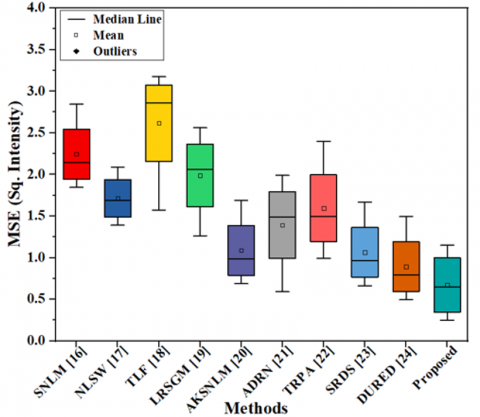
(1) MSE–It is commonly used to quantify the difference between the original and processed images [45]. It is measured in squared intensity values.
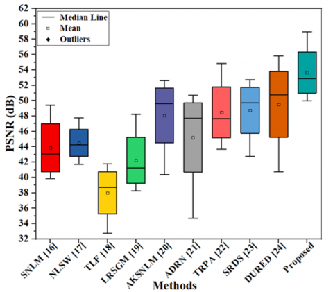
(2) PSNR–It evaluates the quality of a reconstructed or processed image relative to the original by comparing the maximum possible pixel intensity value to the noise introduced during processing [46]. It is measured in Decibels (dB).
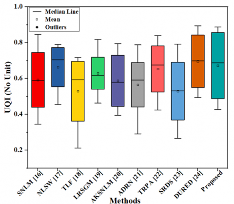
(3) UQI–It measures image quality by considering both structural and luminance similarities between the original and processed images [47]. It does not have a specific unit of measurement.
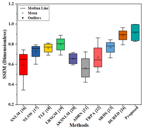
(4) SSIM–It evaluates the perceived quality of a processed image by comparing its structural information, luminance, and contrast with the original image [48]. It is dimensionless.
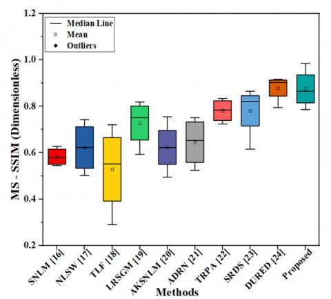
(5) MS-SSIM–It extends SSIM by evaluating parameters like luminance, contrast, and structural similarity across multiple scales. These results are then combined to produce a comprehensive similarity measure [49]. It is also dimensionless.
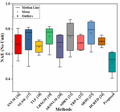
(6) NAE–It provides a normalized measure of the absolute error between the original noisy image and the processed image [50]. It has no units.
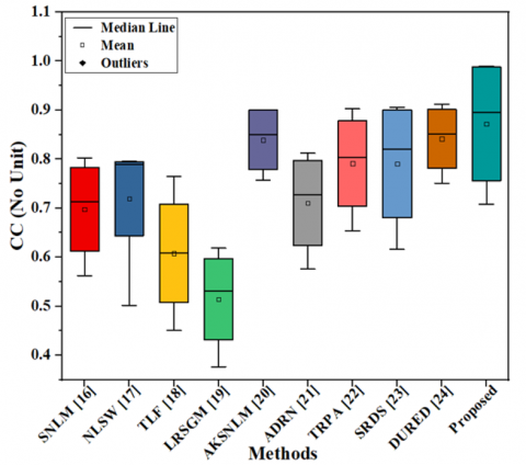
(7) CP/CC–It is a statistical measure that describes the linear relationship between two images [51]. There is no unit associated with it.
(8) DE–It shows the amount of information or randomness in the intensity values of images [52]. It is measured in terms of bits per symbol or bits per pixel.
Table 3 shows a detailed description of the mathematical parameters taken for performance assessment. Table 4 shows a detailed description of symbols used for the mathematical formulation of performance assessment parameters in Table 3. The value of these performance assessment parameters obtained in output images is drawn in box plot form. With the help of a box plot, it is easy to find the spread of the data [53].
Table 3. Mathematical formula of performance assessment parameters
|
Index |
Mathematical Formula |
Expected Value |
|
MSE [45] |
$\frac{1}{P \times N} \sum_{i=1}^{P-1} \sum_{j=1}^{N-1}(M(i, j)-I(i, j))^2$ |
Low |
|
PSNR [46] |
$20 \log _{10} \frac{(L-1)}{\sqrt{M S E}}$ |
High |
|
UQI [47] |
$\frac{4 \mu_M \mu_I \sigma_{M I}}{\left(\mu_M{ }^2+\mu_I{ }^2\right)\left({\sigma_M}^2+\sigma_I{ }^2\right)}$ |
High |
|
SSIM [48] |
$\frac{\left(2 \mu_M \mu_I+C_1\right)\left(2 \sigma_{M I}+C_2\right)}{\left(\mu_M{ }^2+\mu_I{ }^2+C_1\right)\left({\sigma_M}^2+\sigma_I{ }^2+C_2\right)}$ |
High |
|
MS-SSIM [49] |
$\frac{\left(2 \mu_M \mu_I+C_1\right)}{\left(\mu_M^2+\mu_I^2+C_1\right)} \prod_0^{L-1} \frac{\left(2 \sigma_{M I}+C_2\right)}{\left(\sigma_M^2+\sigma_I^2+C_2\right)}$ |
High |
|
NAE [50] |
$\frac{\sum_{i=1}^{P-1} \sum_{j=1}^{N-1}(M(i, j)-I(i, j))}{\sum_{i=1}^{P-1} \sum_{j=1}^{N-1} M(i, j)}$ |
Low |
|
CP [51] |
$\frac{\sum_{i=1}^P \sum_{j=1}^N\left(M(i, j)-\mu_M\right)\left(I(i, j)-\mu_I\right)}{\sqrt{\sum_{i=1}^P \sum_{j=1}^N\left(M(i, j)-\mu_M\right)^2 \sum_{i=1}^P \sum_{j=1}^N\left(I(i, j)-\mu_I\right)^2}}$ |
High |
|
DE [52] |
$-\sum_{i=0}^{L-1} I(i, j) \log _2(I(i, j))$ |
High |
Table 4. Detailed description of symbols taken for the mathematical formulation of assessment parameters
|
Symbol |
Description |
|
$M(i, j)$ |
Noisy MR image. |
|
$I(i, j)$ |
Processed output image. |
|
$(i, j)$ |
Pixel coordinates of image. |
|
$P \times N$ |
Dimension size of the image. |
|
$L$ |
Dynamic possible pixel range of image. |
|
$\mu_M$ |
Mean of reference noisy MR image. |
|
$\mu_I$ |
Mean of processed output MR image. |
|
$\sigma_M$ |
Standard deviation of reference noisy MR image. |
|
$\sigma_I$ |
Standard deviation of processed MR image. |
|
$\sigma_{M I}$ |
Covariance of noisy input and processed image. |
|
$C_1, C_2$ |
Constant taken to prevent the resulting instability. |
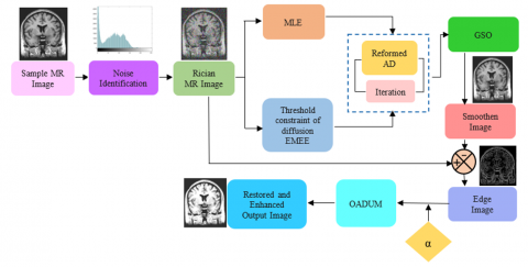
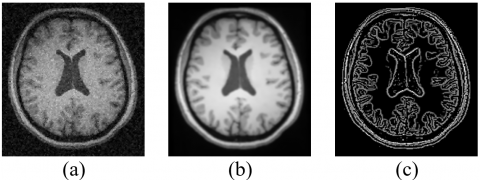
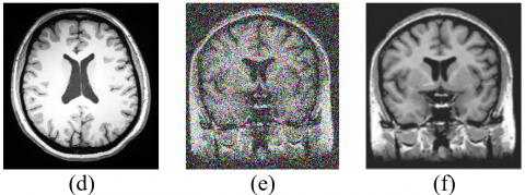
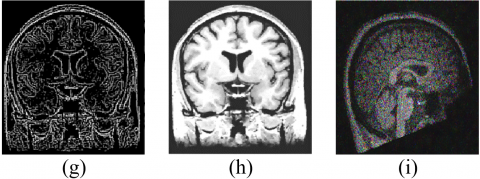
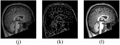
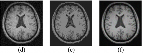
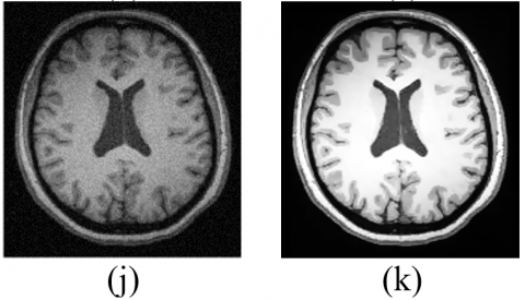
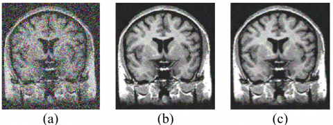
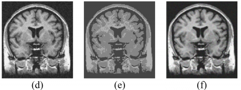
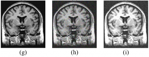
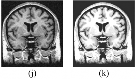
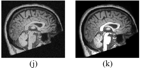
This section shows the findings of the qualitative and quantitative outputs of the proposed methodology. This illustrates the amount of information or randomness present in the intensity values of images. Figure 3 shows the output MR images obtained at each step of the proposed methodology. Figure 3(a), 3(e), and 3(i) show sample Axial, Coronal, and Sagittal scan MR images taken from the dataset, respectively [25]. Figure 3(b), 3(f), and 3(j) represent a smoothen image obtained after optimization. Figures 3(c), 3(g), and 3(k) show the edge image obtained after deducting the smoothed image from the input MR image. Finally, Figures 3(d), 3(h), and 3(l) exhibit a restored and sharpened enhanced image obtained after the proposed methodology. Further, Figures 4-6 show a comparative study of the final output image obtained with the proposed methodology and the earlier existing method discussed in Section II with Axial, Coronal, and Sagittal MR images of the dataset, respectively. In this comparative analysis, it can be seen that the visual output of the proposed methodology is more enhanced and sharper in comparison to earlier existing methods. For a more subjective evaluation, we conducted a comprehensive study involving a diverse group of individuals with expertise in medical imaging, including radiologists, clinicians, and imaging scientists. Finally, based on the recommendations from the doctors of the medical department at the National Institute of Technology Patna, India, the proposed methodology produces a denoised and enhanced MR image that sharpens the details of abnormalities, aiding in the accurate detection of disorders.
Figure 3. MR image (a) Sample axial [25], (b) Smoothen axial, (c) Edge image of axial, (d) Enhanced axial output, (e) Sample Coronal [25], (f) Smoothen Coronal, (g) Edge image of Coronal, (h) Enhanced Coronal output, (i) Sample Sagittal [25], (j) Smoothen Sagittal, (k) Edge image of Sagittal, and (l) Enhanced Sagittal output
Figure 4. (a) Sample axial MR image [25], (b) SNLM [16], (c) NLSW [17], (d) TLF [18], (e) LRSGM [19], (f) AKSNLM [20], (g) ADRN [21], (h) TRPA [22], (i) SRDS [23], (j) DURED [24], and (k) Proposed
Figure 5. (a) Sample coronal MR image [25], (b) SNLM [16], (c) NLSW [17], (d) TLF [18], (e) LRSGM [19], (f) AKSNLM [20], (g) ADRN [21], (h) TRPA [22], (i) SRDS [23], (j) DURED [24], and (k) Proposed
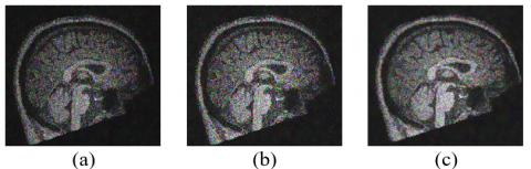
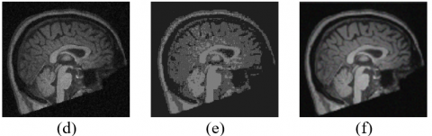
Figure 6. (a) Sample sagittal MR image [25], (b) SNLM [16], (c) NLSW [17], (d) TLF [18], (e) LRSGM [19], (f) AKSNLM [20], (g) ADRN [21], (h) TRPA [22], (i) SRDS [23], (j) DURED [24], and (k) Proposed
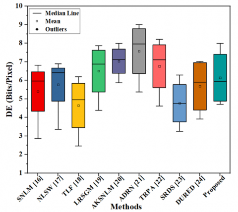
Apart from qualitative analysis, a quantitative analysis of the parameters discussed in Table 3 has also been done in between the proposed method and earlier existing methods. A comparison of the average performance assessment parameters between the earlier existing method and the proposed method is shown in Table 5 for this dataset. It can be observed that the proposed methodology imparts better results, such as a high PSNR ratio, low MSE, higher UQI, SSIM, MS-SSIM, lower NAE, higher CC, and lower DE than earlier existing methods. The marked bold values in Table 5 show the optimal value of the performance metrics. However, the underlined values show the second-best value, and the dotted lines show the third-best value observed for these performance assessment parameters. The box plot of the parameters of evaluation given in Table 5 has been shown in Figure 7.
Table 5. Comparative assessment of earlier work with proposed method on dataset
|
S. No. |
Methods |
MSE |
PSNR |
UQI |
SSIM |
MS -SSIM |
NAE |
CC |
DE |
|
1. |
SNLM [16] |
2.0451 |
41.5897 |
0.5331 |
0.6445 |
0.6277 |
0.8051 |
0.7623 |
5.8160 |
|
2. |
NLSW [17] |
1.5897 |
43.7481 |
0.6547 |
0.7541 |
0.7431 |
0.8127 |
0.7858 |
6.3873 |
|
3 |
TLF [18] |
2.7440 |
37.7412 |
0.5126 |
0.7519 |
0.7203 |
0.6366 |
0.5646 |
4.4289 |
|
4. |
LRSGM [19] |
1.9626 |
40.2513 |
0.6185 |
0.7926 |
0.7157 |
0.7653 |
0.5764 |
6.3763 |
|
5. |
AKSNLM [20] |
0.8886 |
48.6484 |
0.7949 |
0.6187 |
0.6063 |
0.7473 |
0.8998 |
6.8774 |
|
6. |
ADRN [21] |
1.3912 |
46.7031 |
0.7881 |
0.7234 |
0.7146 |
0.8759 |
0.7827 |
7.3678 |
|
7. |
TRPA [22] |
1.3956 |
46.6796 |
0.7247 |
0.8637 |
0.8138 |
0.6378 |
0.8537 |
7.6085 |
|
8. |
SRDS [23] |
0.8658 |
48.7468 |
0.7908 |
0.8439 |
0.8156 |
0.8471 |
0.8953 |
5.2561 |
|
9. |
DURED [24] |
0.6942 |
49.7221 |
0.7917 |
0.9648 |
0.9162 |
0.7511 |
0.9125 |
6.9126 |
|
10 |
Proposed |
0.4486 |
51.9872 |
0.8268 |
0.9947 |
0.9857 |
0.6075 |
0.9862 |
5.0547 |
(a)
(b)
(c)
(d)
(e)
(f)
(g)
(h)
Figure 7. Box plot of comparative parameter assessment for performance evaluation between proposed method and existing state of art (a) MSE, (b) PSNR, (c) UQI, (d) SSIM, (e) MS-SSIM, (f) NAE, (g) CC, and (h) DE
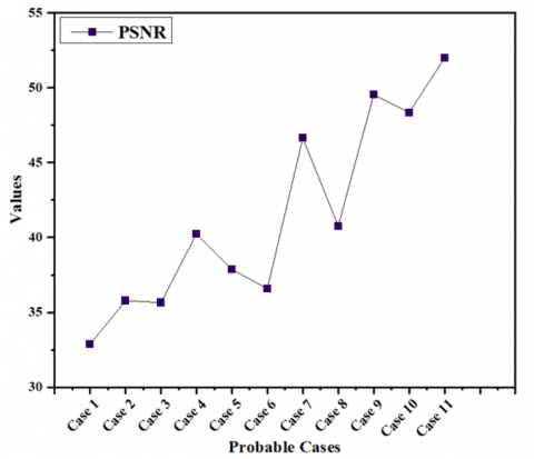
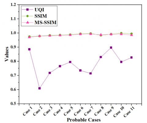
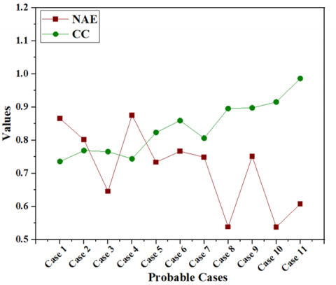
To show the best possible output combination of this method, a total of 11 cases have been taken with the help of random search optimization using the parameters described in Table 2. The values of those iterations are shown in Table 6. The parameters taken for the final output performance assessment calculation are shown in Case 11. A comparative study of these cases is shown with dot plots in Figure 8.
Table 6. Combination of parametric values for finding the best performance assessment parameters on dataset
|
|
Performance Parameters |
|
|
|
|
|
|||||||
|
Experimental Parameter Values |
MSE |
PSNR |
UQI |
SSIM |
MS –SSIM |
NAE |
CC |
DE |
|||||
|
Case 1: |
$\Delta t=0.1, n=02, \beta=10, \alpha$ = 0.5 |
4.9354 |
32.8756 |
0.8846 |
0.9745 |
0.9707 |
0.8657 |
0.7358 |
4.1269 |
||||
|
Case 2: |
$\Delta t=0.2, n=05, \beta=15, \alpha$ = 0.9 |
4.6209 |
35.7754 |
0.6089 |
0.9786 |
0.9782 |
0.8012 |
0.7686 |
4.5275 |
||||
|
Case 3: |
$\Delta t=0.3, n=10, \beta=20, \alpha$ = 1.0 |
4.7428 |
35.6465 |
0.7178 |
0.9836 |
0.9806 |
0.6456 |
0.7655 |
4.2467 |
||||
|
Case 4: |
$\Delta t=0.4, n=15, \beta=25, \alpha$ = 1.2 |
3.1489 |
40.2513 |
0.7656 |
0.9857 |
0.9832 |
0.8754 |
0.7439 |
4.6531 |
||||
|
Case 5: |
$\Delta t=0.5, n=20, \beta=30, \alpha$ = 1.5 |
4.0623 |
37.8761 |
0.7949 |
0.9886 |
0.9854 |
0.7335 |
0.8234 |
4.5738 |
||||
|
Case 6: |
$\Delta t=0.6, n=25, \beta=35, \alpha$ = 1.9 |
4.2954 |
36.5793 |
0.7356 |
0.9945 |
0.9924 |
0.7665 |
0.8592 |
4.7874 |
||||
|
Case 7: |
$\Delta t=0.7, n=30, \beta=40, \alpha$ = 2.0 |
1.4142 |
46.6421 |
0.7144 |
0.9967 |
0.9936 |
0.7488 |
0.8061 |
4.9234 |
||||
|
Case 8: |
$\Delta t=0.8, n=35, \beta=45, \alpha$ = 2.3 |
3.4854 |
40.7468 |
0.8298 |
0.9843 |
0.9876 |
0.5382 |
0.8955 |
5.2095 |
||||
|
Case 9: |
$\Delta t=0.9, n=40, \beta=47, \alpha$ = 2.5 |
0.7246 |
49.5381 |
0.8965 |
0.9921 |
0.9911 |
0.7511 |
0.8976 |
5.2871 |
||||
|
Case 10: |
$\Delta t=1.0, n=45, \beta=50, \alpha$ = 2.7 |
0.8848 |
48.3268 |
0.7956 |
0.9987 |
0.9925 |
0.5376 |
0.9154 |
5.1843 |
||||
|
Case 11: |
$\Delta t=0.1, n=50, \beta=40, \alpha$ = 2.0 |
0.4486 |
51.9872 |
0.8268 |
0.9947 |
0.9857 |
0.6075 |
0.9862 |
5.0547 |
||||
(a)
(b)
(c)
(d)
Figure 8. Dot plot of combination of parameter values taken in all 11 cases (a) PSNR, (b) MSE and DE, and (c) UQI, SSIM, MS-SSIM, NAE, and CC
The major advantage of the proposed method is that it effectively reduces Rician noise in MR images while preserving critical structural details through reformed AD with MLE and EMEE. Parameter optimization via GSO and enhancement using modified UM significantly improve the sharpness and contrast of images, improving both qualitative visual quality and quantitative values, thereby aiding in better diagnosis and clinical applications. Our proposed work and comparison of those works are completely based on traditional image denoising methods; that’s why real-time denoising methods have been omitted. Real-time denoising methods, such as lightweight CNNs, are deep learning models that require a large training dataset to learn effective noise patterns and work aggressively on denoising [54]. Our proposed methodology is robust to small datasets. The proposed method selectively smooths regions based on the edge threshold constant of the diffusion coefficient. It is automated using the Enhancement Measurement on Entropy (EMEE) method and is combined with Maximum Likelihood Estimation (MLE) rather than relying on manual calculation. To further enhance the quality of the smoothed images, the Greedy Search Optimization (GSO) algorithm is employed, with the Peak Signal-to-Noise Ratio (PSNR) serving as the fitness function. This approach facilitates denoising while preserving significant structures, such as edges and contours. In the context of real-time denoising images, it is extremely important to preserve edges rather than solely concentrating on aggressive noise removal. Additionally, real-time denoising methods typically demand more computational resources compared to traditional denoising techniques [55]. Also, in the case of small datasets, these real-time denoising models frequently struggle to generalize effectively because they lack sufficient training samples, resulting in overfitting [56].
Generally, denoising methods are affected by class imbalance, especially when the number of healthy controls in datasets is greater than individuals with abnormalities [57-59]. Model-based or data-driven methods typically learn noise patterns primarily from the majority class [60]. This highlights the importance of balancing the datasets in data-driven denoising methods. To address the issues related to class imbalance, the process of data augmentation is used [61]. Data augmentation increases the number of samples in data using zooming, cropping, rotation, etc., and enhances generalization by introducing diversity into the data. Generative Adversarial Networks (GANs) are the most preferred data augmentation used for balancing the datasets [62]. However, class imbalance does not affect the performance of the proposed method, as it operates independently on each individual image. Also, the main objective of the methodology is to check the ability of the algorithm to improve the quality of the image by removing noise.
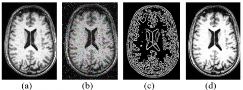
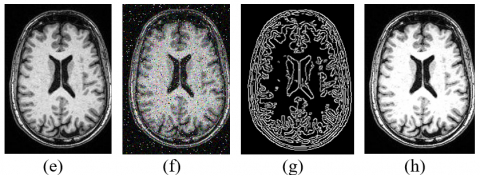
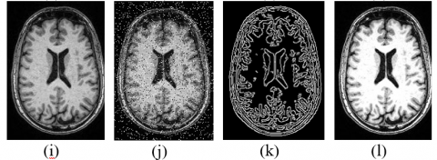
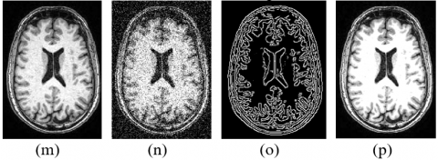
Though the proposed method is tailored for Rician noise. However, its inherent properties that suppresses noise while keeping edges sharp and adjusting the smoothness makes it effective for denoising images affected by Gaussian and Poisson noise too. Some phantom MR images from the Kaggle dataset were taken to support the statement [63]. The proposed methodology has been applied to those images. Figures 9(a), 9(e), 9(i), and 9(m) show sample phantom MR images taken from the dataset [63]. Figures 9(b), 9(f), and 9(j) represent images obtained after adding 5%, 10%, and 20% of Rician noise, respectively. Figures 9(n) comprises a combination of additive Gaussian and Poisson noise. Figures 9(c), 9(g), 9(k), and 9(o) show edge images obtained after deducting the smoothened image from those noisy MR images. Finally, Figures 9(d), 9(h), 9(l), and 9(p) exhibit restored and sharpened enhanced images obtained after the proposed methodology. These noisy images have also undergone a quantitative analysis of the parameters discussed in Table 3. The values of parameter obtained is shown in Table 7. The qualitative and quantitative outputs of the phantom images shows that the proposed method performs well with various other types of noises too.
Figure 9. MR image (a) Phantom image [63], (b) 5% Rician noisy image, (c) Edge image, (d) Enhanced output image, (e) Phantom image [63], (f) 10% Rician noisy image, (g) Edge image, (h) Enhanced output image, (i) Phantom image [63], (j) 20% Rician noisy image, (k) Edge image, (l) Enhanced output image, (m) Phantom image [63], (n) Gaussian and poisson noisy Image, (o) Edge image, and (p) Enhanced output image
Table 7. Quantitative evaluation of the proposed methodology on phantom MR image with different noise variations
|
S. No. |
Noisy Image |
MSE |
PSNR |
UQI |
SSIM |
MS -SSIM |
NAE |
CC |
DE |
|
1. |
Figure 9(b) |
0.5287 |
42.7652 |
0.6684 |
0.8602 |
0.8929 |
0.4941 |
0.8435 |
6.8445 |
|
2. |
Figure 9(f) |
0.6586 |
41.8170 |
0.7515 |
0.8058 |
0.8887 |
0.5367 |
0.8194 |
6.9318 |
|
3. |
Figure 9(j) |
0.4402 |
43.5621 |
0.7461 |
0.7429 |
0.7961 |
0.5801 |
0.7285 |
6.7683 |
|
4. |
Figure 9(n) |
1.2821 |
38.9205 |
0.9735 |
0.8930 |
0.9693 |
0.1730 |
0.9934 |
5.2310 |
Apart from advantages, this methodology has some disadvantage too. This proposed method has high computational complexity and requires precise parameter tuning, which may not always yield optimal results. Additionally, Unsharp Masking can introduce artifacts, and implementing the combined approach requires extensive expertise in image processing. These disadvantages highlight the need for careful consideration and potential improvement of methods when taken for future application in other digital image processing.
The primary objective of this method is to achieve superior visual quality with reducing noise and preserving critical structural details thereby enhancing the features of MR images for diagnostic and clinical applications. The proposed method effectively restores and enhances Rician noise-corrupted MR images by integrating AD for denoising, GSO for parameter optimization, and OADUM for improving the sharpness and contrast of the MR image. The efficiency of the model can be validated through qualitative and quantitative analyses. From the comparative study, it can be seen that the proposed method is giving best visual output MR image of taken dataset.
Through quantitative analysis shown in Table 5., the values of parameter MSE, PSNR, UQI, SSIM, MS-SSIM, NAE, CC, and DE are coming out to be 0.4486, 51.9872, 0.8268, 0.9947, 0.9857, 0.6075, 0.9862, and 5.0547, respectively. Out of eight parameters, this method is giving best output for seven parameters which show its utility in diagnostic and clinical settings, contributing to better diagnosis, treatment planning, and patient outcomes. Also, the qualitative and quantitative output values of the phantom images indicate that the proposed methodology produces good denoised output images for various types of noise as well.
Enhancing computational efficiency for real-time processing and integrating machine learning for automatic parameter adjustment can improve its robustness and practicality. This can be further supported by hardware implementation on platforms like GPUs or FPGAs. Implementing the proposed method on GPUs accelerates parallel processing using computing platforms Open Computing Language (OpenCL) or Compute Unified Device Architecture (CUDA). For FPGAs, the use of pipelined fixed-point architectures alongside custom data dataflows can guarantee high throughput and minimal latency. Optimized memory management and fixed-point computations enhance speed and energy efficiency, making them suitable for embedded devices. Additionally, further enhancing its utility and effectiveness in clinical settings can be achieved by extending its application to multimodality imaging, developing a user-friendly interface, validating on larger datasets, and combining it with other enhancement techniques like deep learning-based super resolution.
[1] Chaitanya, P.S., Satpathy, S.K. (2023). A multilevel De-noising approach for precision Edge-based fragmentation in MRI brain tumor segmentation. Traitement du Signal, 40(4): 1715-1722. https://doi.org/10.18280/ts.400440
[2] Tao, M.J., Lou, J.S., Wang, L. (2022). MRI liver image assisted diagnosis based on improved faster R-CNN. Traitement du Signal, 39(4): 1347-1355. https://doi.org/10.18280/ts.390428
[3] Mohan, J., Krishnaveni, V., Guo, Y. (2014). A survey on the magnetic resonance image denoising methods. Biomed Signal Process Control, 9: 56-69. https://doi.org/10.1016/J.BSPC.2013.10.007
[4] Hamad, R.W., Ismail, M.H., Raed, S. (2024). Efficient MRI image real-time processing using FPGA-based IIR filters. Journal Européen des Systèmes Automatisés, 57(3): 869-876. https://doi.org/10.18280/jesa.570326
[5] Xue, T., Liu, W., Wang, L., Shi, Y., Hu, Y., Yang, J., Li, G., Huang, H., Cui, D. (2024). Extracellular vesicle biomarkers for complement dysfunction in schizophrenia. Brain, 147(3): 1075-1086. https://doi.org/10.1093/BRAIN/AWAD341
[6] Jiang, S., Jia, Q., Peng, Z., Zhou, Q., An, Z., Chen, J., Yi, Q. (2025). Can artificial intelligence be the future solution to the enormous challenges and suffering caused by Schizophrenia? Schizophrenia, 11: 1-16. https://doi.org/10.1038/S41537-025-00583-4
[7] Brain Tumor Symptoms, Causes, and Types. https://miamineurosciencecenter.com/en/conditions/brain-tumors/, accessed on May 28, 2025.
[8] Riya, Gupta, B., Lamba, S.S. (2021). An efficient anisotropic diffusion model for image denoising with edge preservation. Computers & Mathematics with Applications, 93: 106-119. https://doi.org/10.1016/J.CAMWA.2021.03.029
[9] Thazeen, S., Mallikarjunaswamy, S., Siddesh, G.K., Sharmila, N. (2021). Conventional and subspace algorithms for mobile source detection and radiation formation. Traitement du Signal, 38(1): 135-145. https://doi.org/10.18280/ts.380114
[10] Nair, R.R., Ranganathan, S.S. (2024). Classification of lung adenocarcinoma using convolutional neural networks: A bioinformatics approach. Traitement du Signal, 41(2): 999-1007. https://doi.org/10.18280/ts.410240
[11] Verma, K., Srivastava, S., Mishra, R.K. (2025). Unveiling the best edge detection algorithm for brain magnetic resonance imaging: A qualitative and quantitative comparative study. In: Kumar Singh, K., Singh, S., Srivastava, S., Bajpai, M.K. (eds) Machine Vision and Augmented Intelligence. MAI 2023. Lecture Notes in Electrical Engineering, vol 1211. Springer, Singapore. https://doi.org/10.1007/978-981-97-4359-9_71
[12] Tsiaras, V., Maia, R., Diakoloukas, V., Stylianou, Y., Digalakis, V. (2016). Global variance in speech synthesis with linear dynamical models. IEEE Signal Processing Letters, 23(8): 1057-1061. https://doi.org/10.1109/LSP.2016.2580672
[13] Verma, K., Srivastava, S., Mishra, R.K. (2024). Revolutionizing medical image processing through immersive metaverse: A paradigm shift. In 2024 15th International Conference on Computing Communication and Networking Technologies (ICCCNT), Kamand, India, pp. 1-7. https://doi.org/10.1109/ICCCNT61001.2024.10723867
[14] Fan, Y., Wang, L., Wu, W., Du, D. (2021). Cloud/edge computing resource allocation and pricing for mobile blockchain: An iterative greedy and search approach. IEEE Transactions on Computational Social Systems, 8(2): 451-463. https://doi.org/10.1109/TCSS.2021.3049152
[15] Javeed, A., Zhou, S., Liao, Y., Qasim, I., Noor, A., Nour, R. (2019). An intelligent learning system based on random search algorithm and optimized random forest model for improved heart disease detection. IEEE Access, 7: 180235-108043. https://doi.org/10.1109/ACCESS.2019.2952107
[16] Hu, J., Zhou, J., Wu, X. (2016). Non-local MRI denoising using random sampling. Magnetic Resonance Imaging, 34(7): 990-999. https://doi.org/10.1016/J.MRI.2016.04.008
[17] Nguyen, M.P., Chun, S.Y. (2017). Bounded self-weights estimation method for non-local means image denoising using minimax estimators. IEEE Transactions on Image Processing, 26(4): 1637-1649. https://doi.org/10.1109/TIP.2017.2658941
[18] Chang, H.H., Li, C.Y., Gallogly, A.H. (2018). Brain MR image restoration using an automatic trilateral filter with GPU-based acceleration. IEEE Transactions on Biomedical Engineering, 65(2): 400-413. https://doi.org/10.1109/TBME.2017.2772853
[19] Zhang, Y., Yang, Z., Hu, J., Zou, S., Fu, Y. (2019). MRI denoising using low rank prior and sparse gradient prior. IEEE Access, 7: 45858-45865. https://doi.org/10.1109/ACCESS.2019.2907637
[20] Kanoun, B., Ambrosanio, M., Baselice, F., Ferraioli, G., Pascazio, V., Gómez, L. (2020). Anisotropic weighted KS-NLM filter for noise reduction in MRI. IEEE Access, 8: 184866-184884. https://doi.org/10.1109/ACCESS.2020.3029297
[21] Rai, S., Bhatt, J.S., Patra, S.K. (2021). Augmented noise learning framework for enhancing medical image denoising. IEEE Access, 9: 117153-11768. https://doi.org/10.1109/ACCESS.2021.3106707
[22] Hou, R., Li, F., Zhang, G. (2022). Truncated residual based plug-and-play ADMM algorithm for MRI reconstruction. IEEE Transactions on Computational Imaging, 8: 96-108. https://doi.org/10.1109/TCI.2022.3145187
[23] Chung, H., Lee, E.S., Ye, J.C. (2023). MR image denoising and super-resolution using regularized reverse diffusion. IEEE Transactions on Medical Imaging, 42(4): 922-934. https://doi.org/10.1109/TMI.2022.3220681
[24] Huang, P., Zhang, C., Zhang, X., Li, X., Dong, L., Ying, L. (2024). Self-supervised deep unrolled reconstruction using regularization by denoising. IEEE Transactions on Medical Imaging, 43(3): 1203-1213. https://doi.org/10.1109/TMI.2023.3332614
[25] COBRE. http://fcon_1000.projects.nitrc.org/indi/retro/cobre.html, accessed on August 23, 2024.
[26] Gudbjartsson, H., Patz, S. (1995). The Rician distribution of noisy MRI data. Magnetic Resonance in Medicine, 34(6): 910-914. https://doi.org/10.1002/MRM.1910340618
[27] Pankaj, D., Govind, D., Narayanankutty, K.A. (2021). A novel method for removing Rician noise from MRI based on variational mode decomposition. Biomedical Signal Processing and Control, 69: 102737. https://doi.org/10.1016/J.BSPC.2021.102737
[28] Hoskins, R.F. (2011). The Dirac delta function. In Delta Functions (Second Edition), Woodhead Publishing Limited, pp. 26-46. https://doi.org/10.1533/9780857099358.26
[29] Kornilov, M.V. (2020). Maximum likelihood estimation for disk image parameters. IEEE Signal Processing Letters, 27: 1480-1484. https://doi.org/10.1109/LSP.2020.3017371
[30] Yadav, R.B., Srivastava, S., Srivastava, R. (2016). A partial differential equation-based general framework adapted to Rayleigh’s, Rician’s and Gaussian’s distributed noise for restoration and enhancement of magnetic resonance image. Journal of Medical Physics, 41(4): 254-265. https://doi.org/10.4103/0971-6203.195190
[31] Bai, J., Feng, X.C. (2018). Image denoising using generalized anisotropic diffusion. Journal of Mathematical Imaging and Vision, 60: 994-1007. https://doi.org/10.1007/S10851-018-0790-4
[32] Zhao, W., Huang, L., Wang, J., Sun, Z. (2015). Entropy maximisation histogram modification scheme for image enhancement. IET Image Process, 9(3): 226-235. https://doi.org/10.1049/IET-IPR.2014.0347
[33] Celik, T. (2014). Spatial entropy-based global and local image contrast enhancement. IEEE Transactions on Image Processing, 23(12): 5298-5308. https://doi.org/10.1109/TIP.2014.2364537
[34] Gupta, S., Porwal, R. (2016). Appropriate contrast enhancement measures for brain and breast cancer images. International Journal of Biomedical Imaging, 2016(1): 4710842. https://doi.org/10.1155/2016/4710842
[35] Subramani, B., Veluchamy, M. (2020). A fast and effective method for enhancement of contrast resolution properties in medical images. Multimedia Tools and Applications, 79: 7837-7855. https://doi.org/10.1007/S11042-019-08521-0
[36] Li, H., Wu, S., Deng, L., Liu, C., Chen, Y., Chen, H., Yu, H., Dong, M., Zhu, L. (2015). Enhancing infrared and visible image fusion through multiscale Gaussian total variation and adaptive local entropy. The Visual Computer, 41: 7817-7838. https://doi.org/10.1007/S00371-025-03840-W
[37] Huang, Y., Zhao, Y., Capstick, A., Palermo, F., Haddadi, H., Barnaghi, P. (2024). Analyzing entropy features in time-series data for pattern recognition in neurological conditions. Artificial Intelligence in Medicine, 150: 102821. https://doi.org/10.1016/J.ARTMED.2024.102821
[38] Yang, J., Guo, Z., Wu, B., Du, S. (2023). A nonlinear anisotropic diffusion model with non-standard growth for image segmentation. Applied Mathematics Letters, 141: 108627. https://doi.org/10.1016/J.AML.2023.108627
[39] Kumar, A., Kumar, P., Srivastava, S. (2022). A skewness reformed complex diffusion based unsharp masking for the restoration and enhancement of Poisson noise corrupted mammograms. Biomedical Signal Processing and Control, 73: 103421. https://doi.org/10.1016/J.BSPC.2021.103421
[40] Kumar, R., Srivastava, S., Srivastava, R. (2017). A fourth order PDE based fuzzy C-means approach for segmentation of microscopic biopsy images in presence of Poisson noise for cancer detection. Computer Methods and Programs in Biomedicine, 146: 59-68. https://doi.org/10.1016/J.CMPB.2017.05.003
[41] Verma, K., Srivastava, S., Mishra, R.K. (2024). Novel fuzzy type-II driven modified Anisotropic Diffusion filter framework for restoration and enhancement of Rician noise corrupted MR images. Multimedia Tools and Applications, 83: 86621-86655. https://doi.org/10.1007/S11042-024-19624-8
[42] Nose, T. (2016). Efficient implementation of global variance compensation for parametric speech synthesis. IEEE/ACM Transactions on Audio, Speech, and Language Processing, 24(10): 1694-1704. https://doi.org/10.1109/TASLP.2016.2580298
[43] Noroozi, M., Mohammadi, H., Efatinasab, E., Lashgari, A., Eslami, M., Khan, B. (2022). Golden search optimization algorithm. IEEE Access, 10: 37515-37532. https://doi.org/10.1109/ACCESS.2022.3162853
[44] Lai, T., Fujita, H., Yang, C., Li, Q., Chen, R. (2019). Robust model fitting based on greedy search and specified inlier threshold. IEEE Trans Ind Electron, 66: 7956-7966. https://doi.org/10.1109/TIE.2018.2881950
[45] Mishra, H.K., Kaur, M. (2022). An approach for enhancement of MR images of brain tumor. Traitement du Signal, 39(4): 1133-1144. https://doi.org/10.18280/ts.390405
[46] Kumar, P., Srivastava, S., Padma Sai, Y., Choudhary, S. (2021). Optimal Bayesian estimation framework for reduction of speckle noise from breast ultrasound images. In Innovations in Cyber Physical Systems. Lecture Notes in Electrical Engineering, pp. 255-263. https://doi.org/10.1007/978-981-16-4149-7_22
[47] Hou, G., Zhao, X., Pan, Z., Yang, H., Tan, L., Li, J. (2020). Benchmarking underwater image enhancement and restoration, and beyond. IEEE Access, 8: 122078-122091. https://doi.org/10.1109/ACCESS.2020.3006359
[48] Patsariya, S., Dixit, M. (2022). Entropy based secure and robust image watermarking using lifting wavelet transform and multi-level-multiple image scrambling technique. Traitement du Signal, 39(5): 1751-1759. https://doi.org/10.18280/ts.390533
[49] Zhu, Y.B. (2020). Color management of digital media art images based on image processing. Ingénierie des Systèmes d’Information, 25(4): 445-452. https://doi.org/10.18280/isi.250406
[50] Mendo, L. (2009). Estimation of a probability with guaranteed normalized mean absolute error. IEEE Communications Letters, 13(11): 817-819. https://doi.org/10.1109/LCOMM.2009.091128
[51] Jiang, Y. (2021). Application of deep learning and brain images in diagnosis of Alzheimer’s patients. Traitement du Signal, 38(5): 1431-1438. https://doi.org/10.18280/ts.380518
[52] Çiğ, H., Güllüoğlu, M.T., Er, M.B., Kuran, U., Kuran, E.C. (2023). Enhanced disease detection using contrast limited adaptive histogram equalization and multi-objective cuckoo search in deep learning. Traitement du Signal, 40(3): 915-925. https://doi.org/10.18280/ts.400308
[53] Liu, S., Fang, L., Zhou, Z., Hong, Y. (2020). Uncertain box-cox regression analysis with rescaled least squares estimation. IEEE Access, 8: 84769-84776. https://doi.org/10.1109/ACCESS.2020.2989211
[54] Heunis, S., Lamerichs, R., Zinger, S., Caballero-Gaudes, C., Jansen, J.F.A., Aldenkamp, B., Breeuwer, M. (2020). Quality and denoising in real-time functional magnetic resonance imaging neurofeedback: A methods review. Human Brain Mapping, 41(12): 3439-34367. https://doi.org/10.1002/HBM.25010
[55] Juneja, M., Rathee, A., Verma, R., Bhutani, R., Baghel, S., Saini, S.K., Jindal, P. (2024). Denoising of magnetic resonance images of brain tumor using BT-Autonet. Biomedical Signal Processing and Control, 87: 105477. https://doi.org/10.1016/J.BSPC.2023.105477
[56] Nazir, N., Sarwar, A., Saini, B.S. (2024). Recent developments in denoising medical images using deep learning: An overview of models, techniques, and challenges. Micron, 180: 103615. https://doi.org/10.1016/J.MICRON.2024.103615
[57] Thölke, P., Mantilla-Ramos, Y.J., Abdelhedi, H., Maschke, C., et al. (2023). Class imbalance should not throw you off balance: Choosing the right classifiers and performance metrics for brain decoding with imbalanced data. NeuroImage, 277: 120253. https://doi.org/10.1016/J.NEUROIMAGE.2023.120253
[58] Cui, L., Li, D., Yang, X., Liu, C., Yan, X. (2024). A unified approach addressing class imbalance in magnetic resonance image for deep learning models. IEEE Access, 12: 27368-27384. https://doi.org/10.1109/ACCESS.2024.3365544
[59] Sun, Z., Ying, W., Zhang, W., Gong, S. (2024). Undersampling method based on minority class density for imbalanced data. Expert Systems with Applications, 249: 123328. https://doi.org/10.1016/J.ESWA.2024.123328
[60] Afzal, S., Maqsood, M., Nazir, F., Khan, U., Aadil, F., Awan, K.M., Mehmood, I., Song, O. (2019). A data augmentation-based framework to handle class imbalance problem for Alzheimer’s stage detection. IEEE Access, 7: 115528-115539. https://doi.org/10.1109/ACCESS.2019.2932786
[61] Jiang, X., Ge, Z. (2021). Data augmentation classifier for imbalanced fault classification. IEEE Transactions on Automation Science and Engineering, 18(3): 1206-1217. https://doi.org/10.1109/TASE.2020.2998467
[62] Goodfellow, I.J., Pouget-Abadie, J., Mirza, M., Xu, B., Warde-Farley, D., Ozair, S., Courville, A., Bengio, Y. (2014). Generative adversarial nets. Advances in Neural Information Processing Systems. https://papers.nips.cc/paper_files/paper/2014/hash/f033ed80deb0234979a61f95710dbe25-Abstract.html.
[63] human brain phantom MRI dataset. https://www.kaggle.com/datasets/ukeppendorf/frequently-traveling-human-phantom-fthp-dataset?select=1.nii, accessed on June 4, 2025.