Rajeshwaran Kandhasamy*![]() | Gurumoorthy Kambatty Bojan
| Gurumoorthy Kambatty Bojan![]()
© 2025 The authors. This article is published by IIETA and is licensed under the CC BY 4.0 license (http://creativecommons.org/licenses/by/4.0/).
OPEN ACCESS
Electrocardiogram (ECG) signals observed from wearable sensing devices follow a cyclic and continuous pattern for detecting heart-related diseases. Signal processing for medical psychological vital observation identifies the random or irregular rhythms guided by machine learning and artificial intelligence techniques. In this article, a Cross-Interval Continuous Unification Model (CICUM) is introduced to identify such irregular rhythms in continuous observation intervals. This model is backboned by a two-layer neural network for continuity verification and signal correlation. The first layer is used to identify discontinuous sequences between fixed signal sensing intervals. The second layer is responsible for correlating the peak and lower-order signal pulses with the normal and abnormal ECG training inputs. In the first layer, the continuous time interval metric is used to identify discontinuities that are converged using identified signal iterations. In the second layer, the variations between high and low pulses are used to train the neural network for precise abnormal signal detection. Therefore, the proposed model unifies cross intervals and signal correlations between abnormal and normal sequences to detect heart-related diseases from irregular psychological signals. The CICU improves the sequence classification, detection accuracy, and continuity verification by 14.71%, 8.91%, and 11.82% respectively for the maximum sequences.
ECG, heart disease, neural network, rhythm detection, sequence detection
Advancements in wearable technology have revolutionized the acquisition of ECG signals for heart disease detection. These sensors enable continuous monitoring, providing critical data for early diagnosis [1]. Compact and user-friendly, they facilitate non-intrusive tracking of cardiac health. Enhanced with wireless capabilities, they ensure real-time data transmission to healthcare providers. Wearable ECG sensors typically feature high accuracy and reliability, essential for detecting subtle cardiac anomalies [2]. The portability and convenience of these devices encourage widespread adoption. Integration with mobile applications allows for easy access to health metrics. Battery life and comfort are also optimized to ensure prolonged use [3]. As a result, patients can engage in daily activities without disruption. Collecting comprehensive ECG data, these sensors contribute significantly to preventive cardiology. Continuous innovation in sensor technology promises further improvements in diagnostic accuracy. Wearable ECG sensors represent a significant leap toward proactive heart disease management [4, 5].
Processing ECG signals is crucial for identifying irregular heart rhythms, which can indicate serious health issues. Advanced algorithms analyze these signals to detect arrhythmias accurately [6]. Sophisticated filtering techniques eliminate noise, ensuring the clarity of ECG data. Signal segmentation is employed to isolate relevant cardiac cycles. Pattern recognition algorithms then scrutinize these cycles for irregularities [7]. Early detection of arrhythmias allows for timely medical intervention. The processed ECG data can be visualized in various formats for easier interpretation by clinicians [8]. Continuous monitoring and real-time processing facilitate the immediate detection of abnormal rhythms. The technology significantly reduces the risk of stroke and other complications associated with irregular heartbeats [9]. Developments in signal processing enhance the precision and reliability of arrhythmia detection. Implementing these advanced methods in wearable devices further amplifies their utility [10]. Efficient processing ensures that only critical information is flagged, reducing false alarms. Ultimately, ECG signal processing is a vital component in modern cardiac care [11].
Machine learning has transformed ECG signal processing, providing powerful tools for detecting heart diseases. Algorithms trained on vast datasets can identify complex patterns indicative of cardiac conditions. These models improve diagnostic accuracy by learning from diverse ECG signal variations [12, 13]. Feature extraction techniques play a pivotal role in highlighting relevant aspects of the signal. Machine learning algorithms, such as neural networks and support vector machines, are commonly employed. These methods enable the detection of subtle anomalies that might be missed by traditional techniques [14, 15]. Automated analysis reduces the workload on healthcare professionals, allowing them to focus on critical cases. Continuous learning from new data ensures that these models remain up-to-date with emerging cardiac trends [16]. Integration with cloud computing facilitates extensive data processing and storage. The adaptability of machine learning models enhances their application across different patient demographics. Precision and efficiency in detecting heart diseases are significantly boosted [17]. The technologies discussed above leap forward in predictive and preventive cardiology-related issues. To strengthen these discussions, this article contributes the following:
The contributions of the article are: Section 2 discusses the different methods/ techniques proposed by various authors followed by the proposed model description in Section 3. In Section 4 the experimental and comparison analysis results are presented. Section 5 concludes the article with the model’s summary, findings, and future scope.
Parupudi et al. [17] developed a smartphone-enabled deep-learning approach. The model introduces a smartphone-enabled deep learning system for detecting myocardial infarction (MI) from ECG data. The model incorporates transfer learning, global average pooling, and Softmax layers, achieving high accuracy (99.34%). The deployment on Android devices enables cost-effective MI and abnormal heart disease detection in IoT-based healthcare applications.
Ma et al. [18] introduced an application of a convolutional dendrite net for myocardial infarction (MI) detection. The method enhances MI detection speed by converting deep features into shallow feature logic with low computational cost. Key steps include artefact removal, waveform localization, coding via Hilbert curve, and classification using Convolutional Dendrite Net. The method achieves 98.95% accuracy with an average patient detection time of 2.09 ms on the PTB dataset.
Sinha et al. [19] introduced Data Augmented SMOTE Multi-class Classifier (DASMcC). The method preprocesses ECG data and extracts features from 12-lead signals to ensure high-quality input for classification. Data augmentation techniques are employed to enhance the robustness and generalizability of the model during training and testing. The method assesses five classifiers for predicting cardiovascular diseases using metrics such as accuracy, precision, recall, F1 score, and AUC.
Peng et al. [20] proposed an ECG signal segmentation approach. The ST-Res U-net enhances spatiotemporal feature extraction by combining four levels of ST blocks and a Res Path. The method includes denoising preprocessing and integrates a threshold screening algorithm for accurate R-peak localization, ensuring comprehensive signal analysis. Validated on MIT-BIH and CPSC2019 databases, the method achieves high sensitivity (99.76% and 90.01%, respectively).
Huang et al. [21] introduced a Snippet Policy Network (SPN). SPN utilizes deep reinforcement learning to achieve early classification of cardiovascular diseases using varied-length ECG data. Compared to existing methods, SPN enhances precision, recall, F1-score, and harmonic mean metrics by at least 7%, highlighting its improved disease detection capabilities. The method achieves over 80% accuracy in detecting cardiovascular diseases early, demonstrating robust performance.
Rao and Kakollu [22] introduced CB-HDM for classifying heart disease using ECG signals. The method proposes an improved U-net model named ST-Res U-net for enhanced detection of QRS complexes and R-peaks in ECG signals. The technique involves data preprocessing, spatiotemporal feature extraction using ST-Res U-net, and a threshold screening algorithm for accurate R-peak detection. Testing on MIT-BIH, CPSC2019, and PTB-XL databases shows accurate detection of QRS complexes and R-peaks.
Iqbal [23] developed a new deep-learning method to detect cardiovascular diseases early from ECG signals. The method employs a deep convolutional neural network (CNN) fine-tuned with optimized learning rates for analyzing ECG signals. ECG signals are segmented into data sequences, and each sequence is evaluated based on centroid points. A clustering approach efficiently recognizes and classifies minor variations in ECG signal characteristics to enhance detection accuracy.
González et al. [24] estimate heart failure risk using short ECG and long-term HRV data. The method integrates 30-second ECG recordings with sampled long-term Heart Rate Variability (HRV) to improve accuracy in assessing Heart Failure (HF) risk. The combination offers a comprehensive view of cardiac health, leveraging short-term ECG features and long-term HRV trends. To capture the temporal dynamics of long-term HRV data, the authors introduced a novel survival model named TFM-ResNet.
Alamatsaz et al. [25] developed a lightweight hybrid CNN-LSTM model for ECG-based arrhythmia detection. The method preprocesses ECG signals with resampling and baseline wander removal techniques. An 11-layer neural network combines CNN and LSTM architectures to classify arrhythmias and normal rhythms. The DL model effectively classifies diverse ECG signals, demonstrating robust performance and high diagnostic accuracy in arrhythmia detection.
Fatimah et al. [26] proposed ECG arrhythmia detection using Fourier decomposition and machine learning. The method validates its reliability by testing on data from individuals not used in training, ensuring robust generalization across patients. It achieves an impressive F1 score of 89.35% for detecting super ventricular ectopic beats (SVEB), surpassing current benchmarks in accuracy. The method improves AI models for real-world use, making notable strides in detecting arrhythmias.
Goud et al. [27] developed an intelligent optimized framework for heart disease prediction. The Wolf-based Generative Adversarial System (WbGAS) focuses on predicting three classes: Normal Sinus Rhythm, Arrhythmia, and Congestive Heart Failure. Inspired by wolf behavior, the approach optimizes disease classification through feature extraction and model training. The method demonstrates superior performance compared to existing ML-based approaches for disease prediction.
Parveen et al. [28] proposed a one-dimensional residual deep convolutional auto-encoder (1D-RDCAE) model. The model introduces a novel hybrid DL technique combining spatiotemporal feature analysis with ML for accurate ECG heartbeat classification. The approach detects subtle variations in ECG signals that may not be discernible to the human eye. The 1D-RDCAE method extracts features from processed ECG samples to improve accuracy.
Kuila et al. [29] developed an ECG signal classification method using ELM and CNN. The technique utilizes a 12-layer deep one-dimensional Convolutional Neural Network (CNN) combined with an Extreme Learning Machine (ELM) for accurate ECG signal classification. The hybrid approach capitalizes on CNN's feature extraction capabilities and ELM's precise classification strengths. To further improve classification accuracy, the method incorporates a wavelet self-adaptive threshold denoising technique.
Karimulla and Patra [30] predict sudden cardiac death early using advanced heart rate variability features from ECG signals. The study emphasizes early prediction of Sudden Cardiac Death (SCD) by extracting features from Heart Rate Variability (HRV) signals derived from ECG data. Artifact correction is applied to ensure high-quality data for accurate feature extraction. Sequential Forward Selection (SFS) is utilized to identify the most informative subset of features crucial for prediction.
Mishra and Tiwari [31] developed an IoT-enabled heart disease prediction system using three-layer deep learning and meta-heuristic algorithms. IoT devices collect ECG signals from both healthy individuals and those with heart disease. The model utilizes the tunicate swarm algorithm and slime mold algorithm to identify relevant features for accurate heart disease prediction. Implemented in MATLAB, the methodology is validated based on its signal processing and machine learning capabilities.
Gupta et al. [32] proposed a new method to detect arrhythmias in ECG signals. The method utilizes Fractional Wavelet Transform (FrWT) to effectively preprocess non-stationary ECG signals. Yule-Walker Autoregressive Analysis (YWARA) is employed to extract meaningful features related to arrhythmias, leveraging its capability to model time-series data. Principal Component Analysis (PCA) is used to further enhance feature representation and classification accuracy.
Zhang et al. [33] developed a hybrid feature fusion method to classify short ECG segments in IoT-based healthcare systems. The method integrates rich features from convolutional neural networks (CNNs) with precise temporal information like RR intervals. These fused features are inputted into a support vector machine (SVM) classifier for training and testing. Effectiveness is evaluated using the F1-score, which assesses the classifier's balance between precision and recall across all classes.
The advent of machine learning (ML) and artificial intelligence (AI) techniques has further revolutionized the field by enabling more accurate and efficient analysis of signals. However, detecting random or irregular rhythms within these continuous observations presents unique challenges. The challenges include improper differentiation of ECG signal based on frequency and amplitude due to cross-existence in continuous intervals. Classifying such cross-interval ECG spikes remains unresolved due to varying interrupts and increasing sensing time. This results in generating additional variations in detecting the precise abnormality. ECG vitals are accounted with time factor and the variations are to be measured between successive intervals. The methods discussed above rely on monitoring devices such as phones/wearables [17] and segmentation models [20, 23, 33] to distinguish the variations. Fractional models [26, 32] require differential outputs from the observed patterns. The zero level patterns observed are less compatible with the transform models. Feature based approaches [22, 24, 28, 29] requires high level extraction and this relies on diverse assessments for which variation normalization is to be added. To address this issue, the CICUM is introduced. The proposed model assimilates both the regular and irregular signals to differentiate signals based on time and amplitude. Such differentiations are trained using the learning process separately to improve the detection precision.
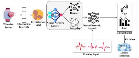
The detection of heart-related diseases has been significantly advanced by the use of Electrocardiogram (ECG) signals obtained from wearable sensing devices. These devices provide continuous and cyclic data crucial for identifying irregular heart rhythms. This article introduces the CICUM, a novel approach designed to enhance the identification of such irregular rhythms in data. It leverages a two-layer neural network structure to ensure continuity verification and precise signal correlation. The proposed unification model is illustrated in Figure 1.
The first layer focuses on detecting discontinuities within fixed sensing intervals, while the second layer correlates signal variations to classify normal and abnormal patterns. This innovative model aims to unify cross-interval data and signal correlations, providing a robust tool for the early detection of heart-related diseases. In ECG monitoring, wearable sensors are designed to detect and record the electrical activity of the heart over extended periods. These sensors provide a stream of continuous data that can be analyzed to detect irregular heart rhythms, making them crucial for early diagnosis and management of heart-related diseases. The collected data by the sensors is transmitted wirelessly to a connected device, where it can be processed. The analysis representation of wearable sensor data is computed in the equation below:
$\begin{array}{r}\left.A=\begin{array}{l}\int_{T_0}^{T_1} W(t) \times X(t), \text { Continuous analysis } \\ \sum_{i=1}^N\left[F_i\left(t_i\right)+G_i\left(t_i\right)\right], \text { Discrete analysis }\end{array}\right\}\end{array}$ (1)
From the above equation, the analysis of observation intervals in wearable sensors is represented as $A$. The continuous analysis focuses on the regular patterns within the sensor data over the observation interval. It integrates the sensor data which is represented as $X(t), W(t)$ is a weighting function to emphasize different parts of the interval based on their significance. The variables $T_0$ and $T_1$ are the start and end times of the observation interval, respectively. The variable $N$ is the total number of discrete analysis points within the interval. Discrete analysis involves the validation of specific irregular points $t_i$ within the intervals. The parameter $F_i\left(t_i\right)$ represents the output of the initial analysis process at specific time points. Another parameter $G_i\left(t_i\right)$ represents the output of the secondary analysis process at the same time points. It combines the outputs from two distinct analysis processes. This component provides detailed insights into specific features or events identified by the analysis processes. This approach allows for a more focused examination of both continuous trends and discrete events within the data, enhancing the understanding and interpretation of complex physiological signals captured by wearable sensors.
Figure 1. Proposed CICU model
Psychological vitals reflect the state of an individual's physical and mental health. These include metrics such as heart rate variability, which can be influenced by stress, and other psychological factors. Monitoring psychological vitals can enhance the detection of irregular heart rhythms by accounting for the influence of psychological stressors on the heart's electrical activity. The below equation P computes the psychological vitals.
$P=\left[\left(\frac{1}{T} \int_{T_0}^{T_1} H(t) d t\right) \times\left(\int_{T_0}^{T_1} B(t) \times Y(t) d t\right)\right]+A$ (2)
Here $H(t)$ represents the baseline heart rate over time. This function can be used to establish a general trend in the heart rate, such as the average heart rate over a specific period. The normalization is observed by the difference in duration $T=$ $T_1-T_0$. Where, $B(t)$ represent the instantaneous heart rate variability which measures the variations in time intervals between consecutive heartbeats. The parameter $Y(t)$ represents another cardiac parameter, such as the amplitude of the ECG signal, which reflects the strength of the heart's electrical activity. It also incorporates the analysis of wearable sensor $A$ which is computed previously. This helps to identify deviations from the norm and indicate abnormal heart rhythms or other cardiac events.
3.1 First layer process
The proposed CICUM considers the wearable sensor input observed in continuous intervals. The neural network segregates regular and irregular intervals in its first layer. The second layer utilizes the training input for feature mapping. Based on the feature, low and high signal unification is performed. If the unification shows up variations, the correlation is identified for disease detection.
The first layer of the neural network in the CICUM model is designed to analyze the ECG signals over continuous time intervals to identify regular and irregular rhythms. This layer utilizes a continuous time interval metric to detect any discontinuities or deviations from the expected rhythmic patterns. By comparing the observed data against established norms, the neural network can pinpoint intervals where the heart's rhythm appears irregular. This process involves sophisticated signal processing techniques and iterative analysis to ensure that even subtle irregularities are detected accurately. The below equation O(t) computes the processes of the first layer of the neural network. Focusing on analyzing heart rhythms based on time and rate of change difference.
$O(t)=\sigma[\Gamma(S(t), \mathcal{F}(S(t)), \Delta S(t))+b]$ (3)
where, $S(t)$ signal at time and $\mathcal{F}(S(t))$ is the Fourier transform of the signal representing frequency components. The computation of $\Delta S(t)$ is the rate of change of signal. The variable $\Gamma$ is the function which computes the difference of rhythms. The variable $b$ represents the bias vector and $\sigma$ activation function. The variable $\bar{S}$ is the mean value of the signal over the interval. The parameter $\overline{\mathcal{F}}$ is the mean value of frequency over the interval. $\overline{\Delta S}$ is the mean value of the rate of change over the interval. The variable $K$ is the number of significant frequency components. $M$ is the number of times considered for the rate of change and $j$ is used to calculate the average rate of change in $S(t)$. The first layer of the neural network intakes $P$ as input for which transform function layer categorizes the baseline and variable $t$. In the first layer process the regular and irregular outputs are identified. Therefore, this first layer contains 3 components in the firsthalf of the architecture. The second layer contains 3 components for classifying $z(t)$ and $O_2(t)$. The pattern matrix layer is responsible for iterating the $\bar{S}$ and $\overline{\Delta S}$. From the above equation, the following equation expands the efficient difference function, reduces complexity, and is scalable for interpretations.
$\left.\begin{array}{c}S(t)=\frac{1}{N} \sum_{i=1}^N\left|S\left(t_i\right)-\bar{S}\right| \\ \mathcal{F}(S(t))=\frac{1}{N} \sum_{K=1}^K\left|\mathcal{F}(S(t))_K-\overline{\mathcal{F}}\right| \\ \Delta S(t)=\frac{1}{M} \sum_{j=1}^M\left|\Delta S\left(t_j\right)-\overline{\Delta S}\right| \\ \text { where } \\ \Delta S\left(t_j\right)=S\left(t_{j+1}\right)-S\left(t_j\right)\end{array}\right\}$ (4)
Here, $\Delta S\left(t_j\right)=S\left(t_{j+1}\right)-S\left(t_j\right)$ measures the difference between consecutive signal values, providing insight into how rapidly the signal is changing. The equation integrates time and frequency components to effectively distinguish between regular and irregular heart rhythms. Neural network provides real-time monitoring and detection of abnormal heart rhythms, facilitating timely medical interventions. The below equation $R_{\text {reg }}(t)$ computes the regular rhythmic pattern over time.
$R_{r e g}(t)=[(S(t)) \times \mathcal{F}(S(t))]<\epsilon_{r e g}$ (5)
The term $S(t)$ calculates the average deviation of the ECG signal from its mean, indicating how much the signal fluctuates around a central value. The variable $\mathcal{F}(S(t))$ measures the stability of the signal's frequency components, ensuring that the signal has consistent periodic transform characteristics. A predefined small threshold is represented as $\epsilon_{\text {reg }}$ ensures that the combined deviations are within acceptable limits for a regular rhythm. Based on regular rhythmic patterns, the below equation computes the irregular rhythmic pattern over time.
$R_{i r-r e g}(t)=\left[R_{r e g}(t) \times \Delta S(t)\right]>\epsilon_{i r-r e g}$ (6)
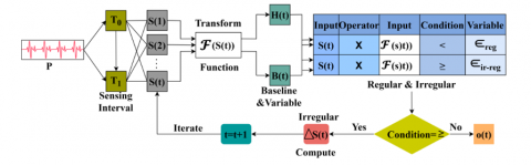
The above equation for irregular rhythm is computed as $R_{\text {ir-reg}}$ indicating the degree of fluctuation in the ECG signals same as the regular rhythm $R_{\text {reg }}(t)$. But in the larger deviations, indicating unstable periodic characteristics. The term $\Delta S(t)$ measures the average rate of change in the ECG signal, capturing sudden changes or erratic behavior. A larger threshold is represented as $\epsilon_{i r-r e g}$ that identifies significant deviations, signalling irregular rhythm. The first layer process is described in Figure 2.
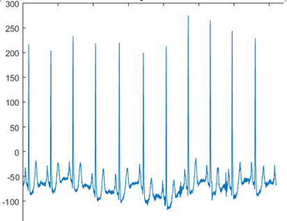
The input P is extracted for $S(1)$ to $S(t)$ that is validated using $\mathcal{F}(S(t))$ to split $\mathrm{H}(\mathrm{t})$ and $B(t)$. This transform function relies on limited to ensure abnormal variations between $T_0$ and $T_1$. If this information is true then $S(t)$ with $\mathcal{F}(S(t))$ is cumulatively analyzed for $2 H(t)$ and $2 B(t)$ variants. In this process, $<$ and $\geq$ conditions are correlated with $\epsilon_{r e g}$ and $\in_{\text {ir-reg}}$ values obtained from clinical observations. If $\geq$ is the condition then the P is irregular and thus $B(t) \geq H(t)$ for which consecutive interval is analyzed. This interval is updated for the $S(t+1)$ to verify $\overline{\Delta S}$. If the condition is $<$ then $o(t)$ is terminated by identifying the outcomes as regular (Refer to Figure 2). For example, in the scenario where the heart signal is monitored for 10 seconds, with the first five seconds showing a regular rhythm and the subsequent five seconds indicating an irregular rhythm, the detection process by the model involves analyzing these temporal patterns. Initially, the model captures and processes the signal for both regular and irregular rhythms separately over the respective time intervals. By comparing these extracted patterns against predefined thresholds, the model determines the presence of irregularities in the heart signal.
$\left.\begin{array}{c}\text { if } \exists_{r e g}>\exists_{i r-r e g} \\ \left.\text { if } \exists_{r e g} \leq \exists_{i r-r e g}\right\}=R(10) \\ \text { where } \\ \exists_{r e g}=\frac{1}{5} \int_0^5 S(t) \times \exp (-\delta t) d t \\ \exists_{i r-r e g}=\frac{1}{5} \int_6^{10} S(t) \times \exp (-\gamma(t-5)) d t\end{array}\right\}$ (7)
The iterative process of detecting irregularities in heart signals over a 10 -second interval is represented as $R(10)$. This equation integrates the heart signal $S(t)$ over the first 5 seconds. This transformation effectively emphasizes earlier parts of the signal more strongly, capturing essential characteristics of regular heart rhythms which are represented as $\exists_{r e g}$. Over the interval from 6 to 10 seconds, the transformation focuses on the latter part of the signal, capturing distinct differences associated with irregular heart rhythms which are denoted as $\exists_{i r-r e g}$. The variables $\delta$ and $\gamma$ are decay constants. In this specific case, detecting an irregular rhythm during the second five-second interval signifies a shift from the normal baseline observed in the first interval, prompting the model to classify the overall signal as irregular. This process highlights the model's ability to dynamically assess temporal changes in heart rhythms, crucial for the accurate detection of irregularities and timely medical intervention. From the analysis of regular and irregular rhythmic patterns, the below formulation computes the condition of rhythmic patterns.
$\left.\begin{array}{c}C_1(t)=R_{r e g}(t) \leq \epsilon_1 \text { highly regular } \\ C_2(t)=\epsilon_1<R_{r e g}(t) \leq \epsilon_2 \text { moderately regular } \\ C_3(t)=\epsilon_2<R_{i r-r e g}(t) \leq \epsilon_3 \text { moderately irregular } \\ C_4(t)=R_{i r-r e g}(t)>\epsilon_3 \text { highly irregular }\end{array}\right\}$ (8)
Figure 2. First layer process illustration for type classification
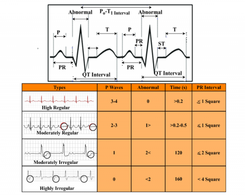
From the above equation, the variable $C_1$ represents the analysis of a very stable heart rhythm with minimal deviations in both time and frequency domains. This derivation set is useful for confirming normal cardiac function. The variable $C_2$ indicates slight variations that are still within acceptable limits. This is for monitoring minor changes in heart rhythm. The representation $C_3$ shows moderate deviations, possibly signaling early signs of cardiac issues. The variable $C_4$ represents significant deviations and instability, suggesting potential serious cardiac events. The network can accurately classify and monitor heart rhythms, facilitating early detection and diagnosis of cardiac conditions. The classifications presented in Eq. (8) are correlated with the conditions in Eq. (7) and are illustrated in Figure 3.
Figure 3. Correlated classifications based on Eqs. (7) and (8)
The above correlation data is obtained from the clinical data correlation used from [34-36]. Based on the information extracted, the P waves, abnormality count in the ($T_0-$ $T_1$) time are presented. Similarly, the visual observation of several PR intervals (i.e.) $M$ and K are defined based on square signals observed in the time interval. Depending on the available $S(t)$ input, the ratio between P and R defines $\epsilon_{\text {reg}}$ and $\overline{\Delta S}$ from which a 10 s interval observation is pursued. Therefore the $\mathcal{F}_{\text {reg}}$ are the $\mathrm{P}, \mathrm{R}$, and M variables observed. The conditions specified in Eq. (7) are validated according to the threshold observed in the accounted time (Refer to Figure 3).
3.2 Second layer process
The second layer of the neural network receives its input from the output generated by the first layer. Essentially, this means that the intervals identified as irregular by the first layer are passed on to the second layer for further analysis. This enhances the precision and efficiency of the overall detection process. This layer uses this input to perform more detailed signal correlation and analysis, aiming to classify the nature of the irregularities identified.
$I(t)=Q \times\left[\begin{array}{c}O_{\text {reg }}(t) \\ O_{\text {ir-reg }}(t) \\ \mathbb{P} \mathrm{q}_{\text {data }}\end{array}\right]$ (9)
This equation combines the outputs from layer 1 as regular and irregular rhythm $O_{r e g}(t)$ and $O_{i r-r e g}(t)$. It also includes pre-trained signal patterns which are represented as $\mathbb{P} q_{\text {data}}$ into a single input vector $I(t)$ through a transformation matrix $Q$. The transformation matrix linearly combines the input vectors, which helps in integrating different aspects of the heart signal, such as regular and irregular patterns. This step prepares the data by mixing the different input sources in a structured way, ensuring that both historical patterns and current observations are considered. The below equation $\mathbb{F}(t)$ computes the classification process of signals.
$\mathbb{F}(t)=\left[\begin{array}{c}\exp \left(I(t)_1 \otimes I(t)_2\right) \\ \log \left(1+\left|I(t)_3\right|\right) \\ \sin \left(I(t)_4\right)\end{array}\right]$ (10)
This equation extracts non-linear classification from the transformed input vector $I(t)$. The term $\exp \left(I(t)_1 \otimes I(t)_2\right)$ applies an exponential function to the element-wise multiplication $\otimes$ of two parts of the input vector which is $I(t)_1$ and $I(t)_2$, capturing multiplicative interactions and emphasizing significant deviations. The term $\log (1+$ $\left.\left|I(t)_3\right|\right)$ applies a transformation, which compresses the range of values and emphasizes smaller variations, making the model sensitive to subtle changes. The term $\sin \left(I(t)_4\right)$ introducing periodicity into the classification set, which is useful for detecting rhythmic patterns in heart signals These transformations are pivotal in capturing nuanced relationships and subtle variations within the heart signals. By emphasizing multiplicative interactions, compressing value ranges, and introducing periodicity, this approach enhances the model's ability to discern complex patterns indicative of potential heart abnormalities. From the classification, the output of the second layer neural network is computed below:
$Z(t)=\mathbb{F}(t)+b_2$ (11)
$O_2(t)=\sigma_2(Z(t))=\left(\prod_{i=1}^N \sigma_2\left(Z_i(t)\right) \times \sqrt{\left|Z_i(t)\right|}\right)$ (12)
Neural network layer 2 contributes significantly to heart signal detection by integrating diverse inputs and applying robust classification criteria. The bias vector which is represented as $b_2$ helps in adjusting the output and providing the model with more flexibility. The intermediate output is represented as $Z(t)$. Here, $\sigma_2$ denoted as activation enabling the model to handle complex relationships in the data. The resulting output of the second layer $O_2(t)$ represents the processed signal indicating the likelihood of high or low signal variations, critical for detecting heart abnormalities. By analyzing the amplitude and frequency of these pulses, the model can differentiate between normal and abnormal heart rhythms. High signals, characterized by significant deviations from the norm, indicate potential abnormalities, while low signals suggest a stable and normal heart rhythm. The below formulation computes the conditions of high and low variations in signal.
$S_2(t)=\left\{\begin{aligned} \mathcal{H}(t) & =\mathbb{I}\left[O_2(t)>\theta_{\text {high }}\right] \\ \mathcal{L}(t) & =\mathbb{I}\left[O_2(t) \leq \theta_{\text {low }}\right]\end{aligned}\right.$ (13)
The variations in signal represented as $S_2(t)$. The indicator function which is denoted as $\mathbb{I}$ produces output as 1 if the condition is true and 0 otherwise. The variable $\theta_{\text {high}}$ is the threshold value for detecting a high signal which is represented as $\mathcal{H}(t)$. The variable $\theta_{\text {low}}$ is the threshold value for detecting a low signal which is denoted as $\mathcal{L}(t)$. These equations serve to classify the output $O_2(t)$ from the neural network layer 2 into high or low signal categories based on variations from predefined thresholds. Figure 4 presents the process of the second neural layer.
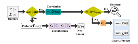
The $\mathrm{O}_2$ (t) process is illustrated in Figure 4 using $\bar{S}$ and $\overline{\Delta S}$ inputs from the layer 1. The 4 different types (i.e.) $C_1$ to $C_4$ be validated using $I(t)$ for $\mathbb{P} q_{\text {data}}$ and Q matrix entries. These entries are validated to find $O_2(t)>O_{\text {high }} \leq$ or $O_{\text {low}}$ outputs. For both the high and low outputs, $Z(t)$ is computed by assigning $b_2$. After assigning $b_2$ the $I(t)$ is updated for P and Q entries using $\mathbb{P} q_{\text {data}}$ and $\mathbb{F}(t)$ processes. Depending on the $\epsilon_{\text {reg }}$ from the computed clinical values the M and K are updated for P and Q. Using the updated values $O_{r e g}$ and $O_{i r-r e g}$ for $O_2(\mathrm{t})$ are classified. The conditions are crucial for heart signal monitoring systems to identify abnormalities. It enables the system to automatically flag instances where the heart signal deviates significantly from normal ranges, prompting further investigation or intervention. The below equation $\mathfrak{D}(t)$ computes detection of heart disease based on the observations of neural network layer 2 .
$\mathfrak{D}(t)=\left(\frac{\mathcal{H}(t)}{\max (\mathcal{H}(t))}\right)+\left(1-\frac{\mathcal{L}(t)}{\max (\mathcal{L}(t))}\right)+\left(\frac{O_2(t)}{\max \left(O_2(t)\right)}\right)$ (14)
The above equation integrates multiple factors crucial in signal analysis to contribute significantly to the detection of heart disease. By incorporating high and low signal classifications $\mathcal{H}(t)$ and $\mathcal{L}(t)$ the equation assesses the prevalence and absence of abnormal heart rhythms, respectively. The detection process is presented in Figure 5.
The second neural network layer is defined using $\mathcal{H}(t)$ and $\mathcal{L}(t)$ outputs from the first neural network. If the $I\left(t_1\right) \otimes I\left(t_2\right)$ is true, then verification of $R(10) R_{\text {ir-reg}}$ is tallied. If the output is true then some abnormalities are observed. This defines heart disease as $C_1$ or $C_2$ or $C_3$ or $C_4$. The correlation range is based on the actual clinical range defined and utilized. The failing $O_2(t)$ are $\mathcal{F}(S(t))$ transformed for nonlinear classification. The $Z(t) \forall R(10)<R_{\text {ir-reg}}$ generates the $(\mathcal{H}(t))$ and $(\mathcal{L}(t))$ narration. Therefore, the detection is performed from $\mathrm{O}_2(t)$ using different first-layer outputs (Figure 5). This approach utilizes these classifications as indicative markers, emphasizing abnormalities that might indicate underlying cardiac issues.
Figure 4. Process of the second neural layer for variation estimation
Figure 5. Detection process illustration
Furthermore, it leverages the output $O_2(t)$ from a neural network layer, which encapsulates variations in heart signals detected through sophisticated data processing. This output serves as a comprehensive indicator of signal anomalies, providing a nuanced assessment of heart health beyond simple classifications.
4.1 Experimental results
This proposed model is validated using an ECG heartbeat categorization data set acquired from the study [37]. In this dataset arrhythmia classification as either normal or abnormal is presented. The abnormal data count is 10k, normal is 4kt, from which 8k inputs are used for training and testing. The samples are observed at 125 Hz frequency, representing 2 categories (normal/abnormal) that correlate with $C_1$ to $C_4$ classifications. The vitals are acquired from 126 subjects classified for arrhythmia and PTB diagnosis. The maximum categories presented are 5, from which 4 are selected for analysis. The classes for analysis range from normal to severe based on the frequency changes between regular intervals. The interval changes from 10s to 60s for abnormal and normal vital observation. The dataset considered in this article provides 5 categories of heart disease classification that suits the unified signal differentiation. Besides the variations across different intervals, define the type of disease for which multiple training input are correlated. These factors are highly correlated with the proposed concept due to which the dataset is found to be apt. The metrics selected are prompt and are adaptable to the concepts provided due to which the comparisons are simplified. Besides, the maximum number of comparison metrics coincides with the existing works which ease the discussion. This information is used to validate the ECG signals through MATLAB experiments. The learning network is trained using 2 batches independently for two layers with a training rate $>0.5$ for both layers. Besides, the number of iterations is 800 $\times 2$ for both layers, such that $C_1$ to $C_4$ classifications are iterated under 3 epochs. These hyperparameter settings are followed in the experimental analysis with linear optimization to enhance the classification and detection processes. The experiments are carried out in a physical standalone computer fixed with 2×16 GB random memory, 25GB storage memory, and a 3.0 GHz clock speed processor. A sample input and output representing the operations of the proposed model are given in Table 1 and Table 2.
Table 1. Sample input and $\mathbb{P} q_{\text {data }}$
|
Input |
$\mathbb{P} \boldsymbol{q}_{\text {data }}$ |
Table 2. Detected output representation
|
$\mathbb{F}(t)$ |
Type |
|
Normal |
|
|
Abnormal |
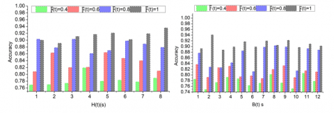
Figure 6. Accuracy analysis under $H(t)$ and $B(t)$ time
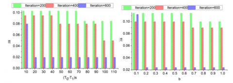
Figure 7. $\overline{\Delta S}$ analysis for $\left(T_0-T_1\right)$ and $b$
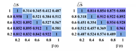
Figure 8. Confusion matrix for $\Delta s$ and $\overline{\Delta S} \forall \mathbb{F}(t)$
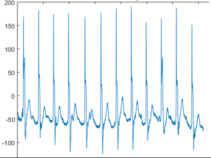
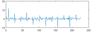
Along with the experiment analysis, the accuracy is analyzed for the $H(t)$ and $B(t)$ under different $\pi$ (t) as presented in Figure 6.
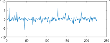
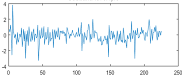
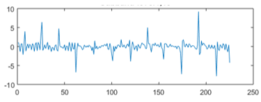
Compared to $B(t)$ the $H(t)$ is a short-lived period using the variable sensors. The challenging process is the $\mathbb{F}(t)$ classification using the two neural network layers. In the first layer, $R_{r e g}(t)$ and $R_{i r-r e g}(t)$ is classified and is iterated based on. This requires a $\overline{\Delta S}$ suppression under limited t. The second layer is responsible for detecting $\mathcal{H}(t)$ and $\mathcal{L}(t)$ between the $\epsilon_{r e g}$ entries. Hence in this case iterations are pursued for $\mathbb{P} q_{\text {data}}$ and $F_i\left(t_i\right)$. In this process the $\overline{\Delta S}$ and b are balanced accordingly to maximize accuracy without the least $\mathbb{F}(t)$ (Figure 6). This process fundamentally relies on $\Delta S$ detection between ($t_0$ and $t_1$) intervals. As the learning iterations increased, the $\overline{\Delta S}$ reduces by mitigating $I(t)$ omissions. This $\Delta S$ analysis b presented in Figure 7 for the ($T_0-T_1$) interval, b, and the increasing iterations.
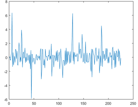
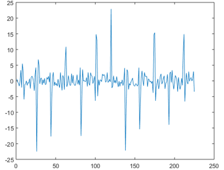
In Figure 7, the $\overline{\Delta S}$ variation suppression under ($T_0-T_1$) and b improvements. As the iterations increase, $\overline{\Delta S}(t)$ and $\geq$ $(t)$ are the iteration-causing factors. This $\overline{\Delta S}$ are variation and high/low sensed information is identified for distinguishable $P$. Thus the $H(t)$ and $B(t)$ differentiations are optimal such that $\sigma$ balances the bias in the $t_i$. Therefore, the two combined layers differentiate the available $\exists_{\text {reg}}$ to identify abnormal and normal P. Thus, this classification is set as a benchmark for reducing $\overline{\Delta S}$ for different $\sigma$ and S. The confusion matrix for $\Delta s$ and $\overline{\Delta S}$ under $\mathbb{F}(t)$ is presented in Figure 8.
The confusion matrix for the ($\Delta s, \Delta S$) pairs under $\mathbb{F}(t)$ is presented in the above Figure 8. The $\exists_{r e g}$ for all $P$ inputs are achieved as differentia table such that the maximum intervention of $\Delta S$ and $\overline{\Delta S}$ are distinguished. In particular, $I\left(t_1\right) \otimes I\left(t_2\right)$ are the verification intensive classifiers such that $\mathcal{H}(t)$ and $\mathcal{L}(t)$ ensures the abnormality detection. The learning for $S_2(t)$ as $\theta_{\text {high}}$ or $\theta_{\text {low}}$ with $b_2$ adjusts the $\mathbb{F}(t)$ such that $O_{r e g}(t)$ and $O_{i r-r e g}(E)$ are the false rate reducing factors. The first layer is responsible for identifying multiple constraints in detecting abnormalities. The learning is referenced through $\mathbb{F}(t)$ provided the transform matrix ensures minimal difference using $\mathbb{P}_{q_{\text {data}}}$. Thus the $\Delta S$ and $\Delta S$ variations for different $\mathbb{F}(t)$ is validated for any $P$ as represented above.
4.2 Comparison results
The comparison results are discussed using sequence classification, detection accuracy, classification time, variation error, and continuity verification metrics. This is analyzed for a varying sensing interval between 10s and 110s for a maximum sequence (/Hr) of 8. To validate the proposed model’s efficacy, it is compared with the 3L-DL+MHA [31], 1D-RDCAE [28], and TFM-ResNet [24] methods from the Section 2.
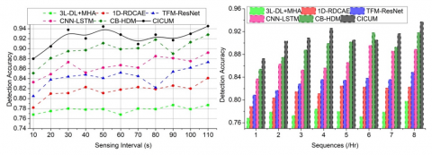
Figure 9. Sequence classification
Figure 10. Detection accuracy
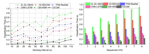
Figure 11. Classification time
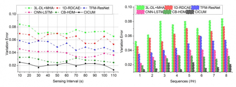
Figure 12. Variation error
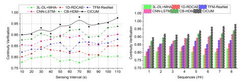
Figure 13. Continuity verification
4.2.1 Sequence classification
Sequence classification refers to the model's ability to distinguish between regular and irregular heart rhythms, which are crucial for accurate heart monitoring. This represents the efficiency in classifying sequences within different sensing intervals, which is computed as $R_{\text {reg }}(t)$ and $R_{\text {ir-reg }}(t)$. The performance is determined by its two-layer neural network architecture. The first layer is designed to detect discontinuous sequences within the fixed signal sensing intervals, using a continuous time interval metric. As the sensing interval increases, the model has more data per sequence, which can improve classification accuracy due to the richer context available for analysis. The second layer focuses on correlating high and low signal pulses with normal and abnormal ECG training inputs. This layer uses the variations between high and low pulses to train the neural network for precise abnormal signal detection, computed as $S_2(t)$. The output from the first layer serves as an input for the second layer, $I(t)$ it to refine its classification based on the identified discontinuities and correlations. This higher classification performance at longer intervals, due to the increased amount of data per sequence, allows the model to make more informed decisions. The ability to maintain high classification standards across different timeframes is highlighted, showcasing its robustness and adaptability in real-time heart monitoring applications (Figure 9).
4.2.2 Detection accuracy
Detection accuracy measures how correctly the model identifies normal and abnormal heart signals. This shows high accuracy across all intervals and sequences, indicating the robustness of the neural network layers. The first layer's ability to identify discontinuous sequences between fixed signal sensing intervals plays a significant role. This layer uses a continuous time interval metric, which converges using identified signal iterations to ensure accurate detection of discontinuities. The formulation of $R(10)$ in which $\exists_{r e g}=$ $\frac{1}{5} \int_0^5 S(t) \times \exp (-\delta t) d t$ and $\exists_{\text {ir-reg }}=\frac{1}{5} \int_6^{10} S(t) \times$ $\exp (-\gamma(t-5)) d t$ computes the detection accuracy. This includes both the first layer's ability to identify discontinuous sequences and the second layer's proficiency in correlating signal pulses. In this detecting an irregular rhythm during the five-second interval signifies a shift from the normal baseline. It was observed in the first interval, prompting the model to classify the overall signal as irregular. This process highlights the model's ability to dynamically detect temporal changes in heart rhythms. High detection accuracy is crucial for reliable heart-related disease detection, and the model's effectiveness in varied temporal contexts (Figure 10).
4.2.3 Classification time
This compares the time taken by the proposed model to classify sequences across different sensing intervals. Classification time is a critical metric, particularly in real-time applications where quick detection is necessary. From the proposed work, $C_1$ represents a very stable heart rhythm with minimal deviations in time. $C_2$ indicate slight variations and $C_3$ shows moderate deviations. $C_4$ represents significant deviations and instability of classifications based on time. However, it aims to maintain low classification times even at longer intervals by optimizing the neural network layers and leveraging efficient signal processing techniques. This balance between speed and accuracy is vital for practical deployment in wearable heart monitoring devices. This demonstrates shorter classification times at shorter sensing intervals, as less data is processed per sequence (Figure 11).
4.2.4 Variation error
This shows (Figure 12) the variation error in the model's predictions across different sensing intervals and sequences. Variation error indicates the discrepancy between the predicted and actual heart signal classifications. Lower variation error signifies higher model reliability. This highlights that the CICUM maintains low variation error across all intervals and sequences, underscoring its robustness. This is achieved through precise training of the neural network layers, where the second layer particularly focuses on minimizing discrepancies in high and low signal variations. The second layer's role in correlating high variation $\mathcal{H}(t)=$ $\mathbb{I}\left[O_2(t)>\theta_{\text {high}}\right]$ and low variation $\mathcal{L}(t)=\mathbb{I}\left[O_2(t) \leq \theta_{\text {low}}\right]$ signal pulses with normal and abnormal ECG training inputs further minimize variation error. Maintains low variation error across all intervals and sequences, underscoring its robustness. This robustness is achieved through precise training of the neural network layers, where the second layer particularly focuses on minimizing discrepancies in high and low signal variations. The low variation error is essential for reliable heart monitoring, as it ensures that the model's predictions are consistent and accurate.
4.2.5 Continuity verification
This measures the effectiveness of the model in verifying the continuity of heart signal data across different sensing intervals. Continuity verification ensures that the heart signal is consistent and free from significant gaps, which is crucial for accurate monitoring. These show high continuity verification across all intervals and sequences, demonstrating the proficiency of the first neural network layer in identifying discontinuous sequences. The computation of $\mathrm{O}_2(t)$ further enhances the model's ability to maintain continuous and consistent heart signal data. By computing $\mathfrak{D}(t)$, high continuity verification is essential for reliable heart monitoring, as it ensures the data integrity necessary for accurate disease detection. This achieves high continuity verification across all intervals and sequences, demonstrating the proficiency of the first neural network layer in identifying discontinuous sequences. High continuity verification is essential for reliable heart monitoring, as it ensures the data integrity necessary for accurate disease detection (Figure 13).
4.3 Analysis
The comparison results are summarized in Table 3 for the sensing interval and Table 4 for sequences (/Hr).
The CICU improves the sequence classification, detection accuracy, and continuity verification by 12.54%, 9.12%, and 11.38%, respectively. This model reduces classification time and variation error by 8.31% and 9.49%, respectively.
The CICU improves the sequence classification, detection accuracy, and continuity verification by 14.71%, 8.91%, and 11.82%, respectively. This model reduces classification time and variation error by 8.12% and 11.53%, respectively.
Table 3. Comparison results for the sensing interval
|
Metrics |
3L-DL+MHA |
1D-RDCAE |
TFM-ResNet |
CNN-LSTM |
CB-HDM |
CICUM |
|
Sequence Classification (%) |
75.08 |
78.81 |
84.43 |
87.13 |
90.86 |
95.089 |
|
Detection Accuracy |
0.787 |
0.841 |
0.873 |
0.892 |
0.928 |
0.9451 |
|
Classification Time (s) |
0.907 |
0.781 |
0.664 |
0.571 |
0.382 |
0.3076 |
|
Variation Error |
0.0654 |
0.053 |
0.0426 |
0.0362 |
0.0246 |
0.01314 |
|
Continuity Verification |
0.805 |
0.852 |
0.881 |
0.903 |
0.939 |
0.9768 |
Table 4. Comparison results for sequences (/Hr)
|
Metrics |
3L-DL+MHA |
1D-RDCAE |
TFM-ResNet |
CNN-LSTM |
CB-HDM |
CICUM |
|
Sequence Classification (%) |
71.45 |
77.37 |
84.57 |
87.84 |
90.81 |
94.432 |
|
Detection Accuracy |
0.798 |
0.823 |
0.849 |
0.889 |
0.918 |
0.9374 |
|
Classification Time (s) |
0.952 |
0.775 |
0.559 |
0.424 |
0.387 |
0.3229 |
|
Variation Error |
0.0843 |
0.0733 |
0.0545 |
0.0424 |
0.0321 |
0.02074 |
|
Continuity Verification |
0.824 |
0.858 |
0.879 |
0.918 |
0.941 |
0.9822 |
The CICUM introduced in this article offered a promising approach to improving the detection of irregular heart rhythms from continuous ECG signals. This model employed a two-layer neural network and addressed the challenges associated with signal discontinuity and correlation of high and low pulse variations. The first layer identified discontinuous sequences to enhance the model's ability to maintain precise differentiations across different intervals. The second layer correlated signal pulses to ensure accurate classification of normal and abnormal rhythms. This dual-layer approach enabled more precise detection of heart-related diseases, making CICUM a valuable addition to the current landscape of medical signal processing technologies. The CICU improves the sequence classification, detection accuracy, and continuity verification by 12.54%, 9.12%, and 11.38%, respectively for the maximum sensing interval.
For real-world applications, the prior classification based on low/ high variation ensures precise disease detection. In the irregular pattern classification process, the classification part ensures concise rhythm detection even for small variations. Depending on the sophisticated inputs, the modification of impact and the layer implication can be followed. Future work may explore the integration of additional physiological signals and the application of this model to other areas of medical diagnosis, further expanding its potential impact on healthcare.
[1] Bhattarai, A., Peng, D., Payne, J., Sharif, H. (2022). Adaptive partition of ECG diagnosis between cloud and wearable sensor net using open-loop and closed-loop switch mode. IEEE Access, 10: 63684-63697. https://doi.org/10.1109/ACCESS.2022.3182704
[2] Hashimoto, Y. (2024). Lightweight and high accurate RR interval compensation for signals from wearable ECG sensors. IEEE Sensors Letters, 8(6): 7003304. https://doi.org/10.1109/LSENS.2024.3398251
[3] Lázaro, J., Reljin, N., Bailón, R., Gil, E., Noh, Y., Laguna, P., Chon, K.H. (2024). Tracking tidal volume from Holter and wearable armband electrocardiogram monitoring. IEEE Journal of Biomedical and Health Informatics, 28(6): 3457-3465. https://doi.org/10.1109/JBHI.2024.3383232
[4] Fang, B., Yu, Z., Zhang, L.B., Teng, Y., Chen, J. (2024). K-B2S+: A one-dimensional CNN model for AF detection with short single-lead ECG waves from wearable devices. Digital Communications and Networks, 11(3): 613-621. https://doi.org/10.1016/j.dcan.2024.05.004
[5] Lee, C.H., Kim, S.H. (2023). ECG measurement system for vehicle implementation and heart disease classification using machine learning. IEEE Access, 11: 17968-17982. https://doi.org/10.1109/ACCESS.2023.3245565
[6] Naeem, A.B., Senapati, B., Bhuva, D., Zaidi, A., Bhuva, A., Sudman, M.S.I., Ahmed, A.E. (2024). Heart disease detection using feature extraction and artificial neural networks: A sensor-based approach. IEEE Access, 12: 37349-37362. https://doi.org/10.1109/ACCESS.2024.3373646
[7] Grisot, R., Laurent, P., Migliaccio, C., Dauvignac, J.Y., Brulc, M., Chiquet, C., Caruana, J.P. (2023). Monitoring of heart movements using an FMCW radar and correlation with an ECG. IEEE Transactions on Radar Systems, 1: 423-434. https://doi.org/10.1109/TRS.2023.3298348
[8] Gour, A., Gupta, M., Wadhvani, R., Shukla, S. (2024). ECG based heart disease classification: advancement and review of techniques. Procedia Computer Science, 235: 1634-1648. https://doi.org/10.1016/j.procs.2024.04.155
[9] Jyothi, P., Pradeepini, G. (2024). Heart disease detection system based on ECG and PCG signals with the aid of GKVDLNN classifier. Multimedia Tools and Applications, 83(10): 30587-30612. https://doi.org/10.1007/s11042-023-16562-9
[10] Golande, A.L., Pavankumar, T. (2024). Electrocardiogram-based heart disease prediction using hybrid deep feature engineering with sequential deep classifier. Multimedia Tools and Applications, 84: 7443-7475. https://doi.org/10.1007/s11042-024-19155-2
[11] Golande, A.L., Pavankumar, T. (2023). Optical electrocardiogram based heart disease prediction using hybrid deep learning. Journal of Big Data, 10(1): 139. https://doi.org/10.1186/s40537-023-00820-6
[12] Pandey, S.K., Shukla, A., Bhatia, S., Gadekallu, T.R., Kumar, A., Mashat, A., Janghel, R.R. (2023). Detection of arrhythmia heartbeats from ECG signal using wavelet transform-based CNN model. International Journal of Computational Intelligence Systems, 16(1): 80. https://doi.org/10.1007/s44196-023-00256-z
[13] Butler, L., Karabayir, I., Kitzman, D.W., Alonso, A., Tison, G.H., Chen, L.Y., Akbilgic, O. (2023). A generalizable electrocardiogram-based artificial intelligence model for 10-year heart failure risk prediction. Cardiovascular Digital Health Journal, 4(6): 183-190. https://doi.org/10.1016/j.cvdhj.2023.11.003
[14] Nishikimi, R., Nakano, M., Kashino, K., Tsukada, S. (2024). Variational autoencoder–based neural electrocardiogram synthesis trained by FEM-based heart simulator. Cardiovascular Digital Health Journal, 5(1): 19-28. https://doi.org/10.1016/j.cvdhj.2023.12.002
[15] Prusty, M.R., Pandey, T.N., Lekha, P.S., Lellapalli, G., Gupta, A. (2024). Scalar invariant transform based deep learning framework for detecting heart failures using ECG signals. Scientific Reports, 14(1): 2633. https://doi.org/10.1038/s41598-024-53107-y
[16] Fradi, M., Khriji, L., Machhout, M. (2022). Real-time arrhythmia heart disease detection system using CNN architecture based various optimizers-networks. Multimedia Tools and Applications, 81(29): 41711-41732. https://doi.org/10.1007/s11042-021-11268-2
[17] Parupudi, V.S., Panda, A.K., Tripathy, R.K. (2023). A smartphone-enabled deep learning approach for myocardial infarction detection using ECG traces for IoT-based healthcare applications. IEEE Sensors Letters, 7(11): 7006704. https://doi.org/10.1109/LSENS.2023.3328593
[18] Ma, X., Fu, X., Sun, Y., Wang, N., Gao, Y. (2022). Application of convolutional dendrite net for detection of myocardial infarction using ECG signals. IEEE Sensors Journal, 23(1): 460-469. https://doi.org/10.1109/JSEN.2022.3221779
[19] Sinha, N., Kumar, M.G., Joshi, A.M., Cenkeramaddi, L.R. (2023). DASMcC: Data augmented SMOTE multi-class classifier for prediction of cardiovascular diseases using time series features. IEEE Access, 11: 117643-117655. https://doi.org/10.1109/ACCESS.2023.3325705
[20] Peng, X., Zhu, H., Zhou, X., Pan, C., Ke, Z. (2023). ECG signals segmentation using deep spatiotemporal feature fusion U-Net for QRS complexes and R-peak detection. IEEE Transactions on Instrumentation and Measurement, 72: 1-12. https://doi.org/10.1109/TIM.2023.3241997
[21] Huang, Y., Yen, G.G., Tseng, V.S. (2022). Snippet policy network for multi-class varied-length ECG early classification. IEEE Transactions on Knowledge and Data Engineering, 35(6): 6349-6361. https://doi.org/10.1109/TKDE.2022.3160706
[22] Rao, C.L.N., Kakollu, V. (2024). CB-HDM: ECG signal based heart disease classification using convolutional block attention assisted hybrid deep Maxout network. Biomedical Signal Processing and Control, 95: 106388. https://doi.org/10.1016/j.bspc.2024.106388
[23] Iqbal, J.M. (2024). A novel deep learning approach for early detection of cardiovascular diseases from ECG signals. Medical Engineering & Physics, 125: 104111. https://doi.org/10.1016/j.medengphy.2024.104111
[24] González, S., Yi, A.K.C., Hsieh, W.T., Chen, W.C., Wang, C.L., Wu, V.C.C., Chang, S.H. (2024). Multi-modal heart failure risk estimation based on short ECG and sampled long-term HRV. Information Fusion, 107: 102337. https://doi.org/10.1016/j.inffus.2024.102337
[25] Alamatsaz, N., Tabatabaei, L., Yazdchi, M., Payan, H., Alamatsaz, N., Nasimi, F. (2024). A lightweight hybrid CNN-LSTM explainable model for ECG-based arrhythmia detection. Biomedical Signal Processing and Control, 90: 105884. https://doi.org/10.1016/j.bspc.2023.105884
[26] Fatimah, B., Singhal, A., Singh, P. (2024). ECG arrhythmia detection in an inter-patient setting using Fourier decomposition and machine learning. Medical Engineering & Physics, 124: 104102. https://doi.org/10.1016/j.medengphy.2024.104102
[27] Goud, P.S., Sastry, P.N., Sekhar, P.C. (2024). A novel intelligent deep optimized framework for heart disease prediction and classification using ECG signals. Multimedia Tools and Applications, 83(12): 34715-34731. https://doi.org/10.1007/s11042-023-16850-4
[28] Parveen, N., Gupta, M., Kasireddy, S., Ansari, M.S.H., Ahmed, M.N. (2024). ECG based one-dimensional residual deep convolutional auto-encoder model for heart disease classification. Multimedia Tools and Applications, 83(25): 66107-66133. https://doi.org/10.1007/s11042-023-18009-7
[29] Kuila, S., Dhanda, N., Joardar, S. (2023). ECG signal classification to detect heart arrhythmia using ELM and CNN. Multimedia Tools and Applications, 82(19): 29857-29881. https://doi.org/10.1007/s11042-022-14233-9
[30] Karimulla, S., Patra, D. (2024). An optimal methodology for early prediction of sudden cardiac death using advanced heart rate variability features of ECG signal. Arabian Journal for Science and Engineering, 49(5): 6725-6741. https://doi.org/10.1007/s13369-023-08457-6
[31] Mishra, J., Tiwari, M. (2024). IoT-enabled ECG-based heart disease prediction using three-layer deep learning and meta-heuristic approach. Signal, Image and Video Processing, 18(1): 361-367. https://doi.org/10.1007/s11760-023-02743-4
[32] Gupta, V., Mittal, M., Mittal, V. (2022). A novel FrWT based arrhythmia detection in ECG signal using YWARA and PCA. Wireless Personal Communications, 124: 1229-1246. https://doi.org/10.1007/s11277-021-09403-1
[33] Zhang, X., Jiang, M., Wu, W., de Albuquerque, V.H.C. (2023). Hybrid feature fusion for classification optimization of short ECG segment in IoT based intelligent healthcare system. Neural Computing and Applications, 35: 22823-22837. https://doi.org/10.1007/s00521-021-06693-1
[34] ECG Abnormalities. https://almostadoctor.co.uk/encyclopedia/ecg-abnormalities, access on Jun. 25, 2024.
[35] What is an ECG? https://www.capitalheart.sg/what-does-an-abnormal-ecg-mean/, access on Jun. 25, 2024.
[36] Sahoo, P.K., Thakkar, H.K., Lin, W.Y., Chang, P.C., Lee, M.Y. (2018). On the design of an efficient cardiac health monitoring system through combined analysis of ECG and SCG signals. Sensors, 18(2): 379. https://doi.org/10.3390/s18020379
[37] ECG Heartbeat Categorization Dataset. https://www.kaggle.com/datasets/shayanfazeli/heartbeat, access on Jun. 25, 2024.