Hatice Kupeli![]() | Ibrahim Kuru
| Ibrahim Kuru![]() | Kerim Kursat Cevik*
| Kerim Kursat Cevik*![]() | Ahmet Bozkurt
| Ahmet Bozkurt![]()
© 2025 The authors. This article is published by IIETA and is licensed under the CC BY 4.0 license (http://creativecommons.org/licenses/by/4.0/).
OPEN ACCESS
This study investigates the efficacy of You Only Look Once (YOLO) algorithms in detecting coronary artery stenosis from angiographic images. The dataset utilized comprises 8,325 grayscale images sourced from publicly available databases, featuring patients diagnosed with single-vessel coronary artery disease. An expert cardiologist annotated the images to precisely mark areas of vascular occlusion, providing reliable training data. Four distinct datasets were constructed and divided into training (80%) and testing (20%) subsets. YOLO v5, v7, and v8 models were trained over 100 epochs to evaluate their performance in identifying stenotic regions. The study emphasizes the advantages of YOLO algorithms, particularly their ability to detect multiple objects in real-time with high accuracy, due to their single-stage detection architecture. Performance metrics such as Mean Average Precision (MAP), precision, recall, and F1-score were computed to assess model effectiveness. The results demonstrate that YOLO v5 and YOLO v8 provide robust detection capabilities, outperforming YOLO v7, especially in complex image scenarios. This research highlights the potential integration of YOLO models in clinical workflows, offering a rapid and accurate tool for automated analysis of coronary artery stenosis.
You Only Look Once (YOLO), coronary artery stenosis, angiographic images, deep learning
Cardiovascular disorders (CVD) encompass a wide range of diseases affecting the heart and blood vessels, primarily caused by factors such as physical inactivity, poor diet, hypertension, smoking, or excessive alcohol consumption [1]. A key consequence of these factors is the buildup of plaque inside the arteries, leading to a condition known as atherosclerosis, where the arterial walls harden and narrow. This narrowing restricts blood flow, often resulting in vascular blockages within the coronary arteries. If left untreated, it can cause serious complications, ranging from chest discomfort to life-threatening heart attacks [2].
Globally, CVDs are among the leading causes of death, responsible for approximately 32% of all fatalities annually, according to the World Health Organization [3]. While CVD-related deaths are lower in high-income countries, the number of fatalities continues to rise in low- and middle-income nations, with predictions indicating that CVD deaths will increase to 22.2 million by 2030 [4]. This trend underscores the critical importance of early diagnosis and timely treatment to reduce mortality rates and improve patient outcomes [5].
A variety of diagnostic methods exist to assess cardiovascular health and identify underlying causes of CVD. These methods range from non-invasive techniques like echocardiography and stress tests to more advanced imaging modalities such as coronary computed tomography (CT), cardiac magnetic resonance imaging (MRI), myocardial perfusion scintigraphy (MPS), radionuclide ventriculography (MUGA), and positron emission tomography (PET) [6]. Among these, x-ray coronary angiography (XCA) has gained popularity due to its precision in visualizing coronary artery health [7].
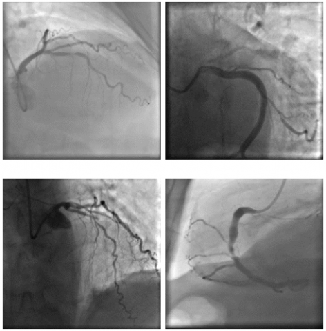
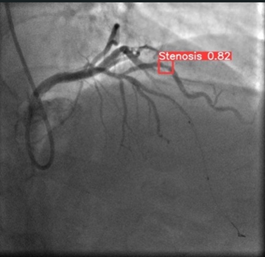
XCA is particularly beneficial in diagnosing coronary artery stenosis (CAS), a condition characterized by the narrowing of the coronary arteries due to plaque buildup [8]. The procedure involves inserting a catheter through the femoral artery into the heart, followed by the injection of contrast material to visualize the coronary vessels. Meanwhile, the pressures inside the heart are monitored, and its contractile function is tested by introducing contrast material into the left ventricle. Following the examination, 4-6 hours of bed rest are usually recommended. Typically, XCA provides high-resolution images, like the ones shown in Figure 1 [9], that allow physicians to detect stenotic areas in coronary arteries and evaluate their severity.
Figure 1. Coronary angiography images and areas of stenosis for a CAS patient [9]
Studying CAS is vital for understanding disease mechanisms, preventing serious cardiac events, enhancing patient care, and improving diagnostic methods. Despite its effectiveness, the manual interpretation of angiography images by experts is often subject to human error, variability, and limitations in time and data processing [10]. As a result, artificial intelligence (AI) has emerged as a powerful tool for enhancing diagnostic accuracy and efficiency. Particularly AI-based techniques employing convolutional neural networks (CNNs) and deep learning (DL) algorithms have demonstrated superior performance over traditional machine learning (ML) approaches in the detection, segmentation, and classification of CAS [11-13].
Research efforts targeting the detection of coronary artery stenosis (CAS) from XCA images have employed various machine learning and deep learning techniques, each presenting unique strengths and limitations. Early approaches like the work of Sameh et al. [14] utilized traditional machine learning methods such as the K-Nearest Neighbor classifier to categorize arterial lumen diameters as normal or pathological, achieving a notable accuracy of 94.6%. Similarly, Wan et al. [15] used an automated Hessian-based method to detect CAS from XCA images and 267 vascular segment sets, reporting a balanced performance with 93.93% accuracy, 91.03% sensitivity, and 93.83% specificity. These foundational works highlighted the utility of machine learning in CAS detection, particularly in assessing lumen diameter and vascular segments, but were limited by their reliance on traditional classifiers.
Deep learning techniques have since dominated the field, providing more robust and automated solutions for CAS detection, segmentation, and classification. Antczak and Liberadzki [16] introduced a Very Deep Convolutional Neural Network (VGG) with five convolutional layers for stenosis detection, supplemented by a Bezier-based generative model that boosted the model’s performance to 90% accuracy. This approach demonstrated the potential of deep neural networks in the task, although it remained constrained by the need for pre-training and synthetic data. More recent work by Wu et al. [17] proposed a two-stage deep learning system combining a UNet model for segmentation and a VGG network for classification of XCA images, which outperformed previous methods with a sensitivity of 87.2% and a positive predictive value of 79.5%. Such studies have shown the efficacy of convolutional neural networks (CNNs) in overcoming the limitations of manual feature extraction, but they often require complex architectures and long training times.
Recent advancements have focused on refining deep learning architectures and improving model efficiency. Danilov et al. [18] explored the use of Faster-RCNN models with various backbone networks, reporting significant results in both prediction time and accuracy. They used three distinct AI models (SSD MobileNet V1, Faster-RCNN ResNet-50 V1, and Faster-RCNN NASNet) to classify and locate stenosis from XCA images. The study found that Faster-RCNN NASNet had the shortest prediction time, with an average processing time of 880 ms, whereas Faster-RCNN ResNet-50 V1 had the largest prediction accuracy. In a similar study, Danilov et al. [9] analyzed clinical angiography data of 100 patients using MobileNet, ResNet-50, ResNet-101, Inception ResNet, and NASNet architectures. They stated that SSD MobileNet V2, despite its lesser accuracy value, was the fastest model. The study by Pang et al. [19] used DetNet to detect CAS, yielding an accuracy of 94.87% and highlighting the growing trend toward model optimization for faster, more accurate detection.
In another study, Ovalle-Magallanes et al. [20] developed a novel Hierarchical Bezier-based Generative Model (HBGM) to generate realistic synthetic XCA patches and enhance training of a convolutional neural network (CNN) for identifying CAS. The study employed an artificial data set of 10,000 images, half with stenosis and half without. The findings indicated an accuracy, precision, and F1 score of 0.8934, 0.9031, 0.8746, 0.8880, and 0.9111, respectively, that were superior than those achieved using pre-trained models. They also classified stenosis on XCA images using the Lightweight Residual Squeeze-and-Excitation Network (LRSE-Net) model [21] by training the model with the Deep Stenosis Detection Dataset and the Angiographic Dataset which resulted in the highest accuracy rate of 0.9549, sensitivity of 0.8792, precision of 0.8944, and F1 score of 0.6103. Meanwhile, hybrid models, like the CNN-Transformer approach developed by Han et al. [22], further enhanced detection accuracy with an F1 score of 90.88%.
The literature demonstrates that XCA imaging plays a crucial role in diagnosing CAS, with accurate identification of stenotic patterns being essential for early intervention. Despite the widespread use of XCA images in classification and segmentation tasks, existing deep learning and machine learning models often face challenges due to the intricate structures of the vascular system. Moreover, achieving high accuracy using single-frame images or snapshots is particularly difficult, as these models struggle to fully capture the complexities of the arterial network. This limitation restricts their overall performance and highlights the need for more effective real-time detection approaches.
In recent years, various deep learning models, including Faster-RCNN, UNet, and VGG networks, have been widely used for detecting CAS from medical images. However, these models often require multiple stages of processing, including region proposal and feature extraction, which can significantly increase computation time and reduce real-time applicability [17, 18]. In contrast, the You Only Look Once (YOLO) algorithm, particularly in its recent versions (v5, v7, and v8), offers significant advantages in terms of speed and efficiency. Unlike traditional models that perform detection in multiple stages, YOLO's architecture allows it to simultaneously predict bounding boxes and classify objects in a single pass through the neural network, which significantly reduces inference time [23, 24]. This capability makes YOLO particularly well-suited for real-time applications in clinical settings, where rapid and accurate decision-making is crucial. Additionally, the recent versions of YOLO have incorporated advanced techniques like CSPNet and the C2f module, which enhance feature extraction and detection accuracy, making it a powerful tool for complex medical image analysis tasks [25].
Existing models often prioritize either accuracy or speed, but not both simultaneously. This trade-off highlights a critical gap in the literature, paving the way for the application of algorithms like YOLO, which is known for its real-time object detection capabilities. In this context, the application of YOLO represents a promising path for addressing the need for rapid and accurate CAS detection from XCA images [23]. YOLO’s ability to detect multiple objects in a single pass and its balance between detection speed and accuracy make it a candidate for analyzing XCA images in real-time, potentially enhancing the diagnostic workflow for CAS [26].
This study addresses these gaps by focusing on the detection of stenotic lesions from both real-time streaming and single-frame angiography images. In contrast to many previous models that primarily rely on static snapshots, we emphasize on the advanced capabilities of the YOLO architecture, which is specifically designed for real-time object detection. By evaluating different versions of YOLO, this study contributes to the literature by exploring its potential for faster, more accurate CAS detection, offering a promising solution to the challenges identified in prior research.
In this study, we employed the YOLO algorithm for detecting coronary artery stenosis (CAS) from X-ray coronary angiography (XCA) images. YOLO was chosen for its ability to simultaneously detect and classify stenotic regions in XCA images.
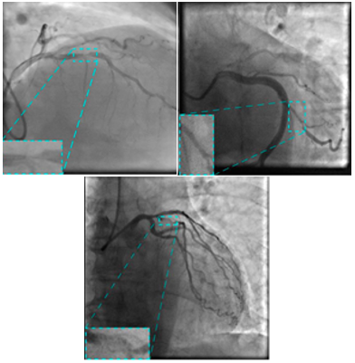
The image dataset utilized in this study was sourced from a publicly available repository provided by Danilov et al. [9]. The images, similar to those given in Figure 2, were captured using high-end imaging systems, namely the Coroscope (Siemens) and Innova (GE Healthcare), which are widely used in clinical practice for precise visualization of coronary arteries.
The dataset comprised angiographic scans from 100 patients, each of whom had been clinically diagnosed with single-vessel coronary artery disease, either through functional assessments or direct angiographic evaluation. The dataset featured a total of 8,325 grayscale images, with resolutions ranging from 512×512 to 1000×1000 pixels, ensuring detailed visualization of the vascular structures. These high-quality images provided an excellent basis for training and evaluating deep learning models, particularly for detecting stenotic regions. Details of each step employed for detecting CAS from XCA images are provided below and are depicted in Figure 3.
The images were extracted from full angiographic video sequences recorded at 15 frames per second. Each angiographic acquisition followed standard imaging protocols involving contrast agent injection under fluoroscopic guidance. The primary imaging systems used were Coroscope (Siemens) and Innova (GE Healthcare), both of which are widely adopted in clinical settings for high-fidelity coronary imaging. Annotations were carried out by a board-certified interventional cardiologist using the open-source VIA tool, with lesions showing ≥50% diameter narrowing labeled as stenotic regions. Annotation standards were based on clinical angiographic interpretation guidelines, and all labels were saved in JSON format. This process ensured the clinical reliability and reproducibility of the dataset used in training and evaluation [9].
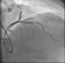
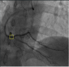
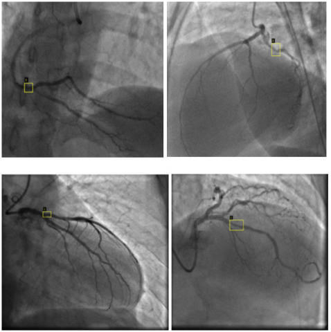
Before employing the images in the YOLO model, vascular occlusions in each XCA image were first identified, and the locations of stenosis were labeled by an expert cardiologist. This crucial step ensured that the dataset was accurate and aligned with clinical standards. For the labeling process, an online annotation tool called VIA (VGG Image Annotator) was utilized [27]. VIA allowed for precise annotation of the stenotic regions, using the existing data values in the supplied dataset to guide the labeling process while preserving the expert’s original decisions without alteration. Each labeled image was then saved in a JSON file format, containing detailed information about the occlusion locations and corresponding metadata. Figure 4 illustrates examples of the labeled images, demonstrating how the stenotic regions were highlighted for further processing. This thorough labeling process was essential for training the YOLO model to accurately detect and classify coronary artery stenosis.
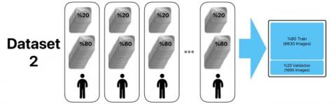
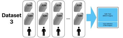
The labeled images were subsequently detected and classified using different versions of the YOLO approach. For the study, four distinct datasets were prepared, each containing all 8,325 images from the original dataset. To ensure robust training and validation, 80% of the images were reserved for training and 20% for testing in each dataset. In the first dataset, the images were randomly assigned, with 6,660 images used for training and 1,665 for testing. For the other datasets, the naming convention of the original dataset ("ID_xxx_x_xxxx") was utilized, where 'x' represents an integer number. In the second dataset, images were grouped based on the first part of the filename (“ID_xxx”), which corresponded to 214 distinct IDs. This resulted in 6,630 images in the training set and 1,695 in the testing set. For the third dataset, the images were selected based on the “ID_xxx_x” element of the filename, representing a more granular grouping of 64 unique IDs. Lastly, the fourth dataset grouped images by the full filename structure ("ID_xxx_x_xxxx"), also corresponding to 64 unique IDs, ensuring a more precise division of the data.
Figure 2. Sample angiography images included in the data set [9]
(a) XCA Images
(b) Labeling
(c) YOLO (v5, v7, v8)
(d) Testing
Figure 3. Process steps employed for detecting CAS of the study
Figure 4. Sample labeled images
These datasets, prepared through different grouping methodologies to explore their impact on model performance, were used to train and test YOLO v5, YOLO v7, and YOLO v8 models. The detailed preparation methodology and resulting dataset compositions are illustrated in Figure 5, showcasing the systematic approach to ensure balanced data distribution for evaluating the effectiveness of the YOLO models.
YOLO architecture [23] employed in this study is a state-of-the-art deep learning (DL) model, designed for real-time object detection and widely adopted in medical imaging tasks. Deep learning itself is a subset of machine learning (ML) that seeks to emulate human cognitive abilities by teaching computers to recognize patterns and execute tasks using data [28]. Unlike traditional ML algorithms, DL models require vast amounts of data and their complex structure necessitates powerful computational hardware [29]. This allows DL algorithms to autonomously identify unique characteristics (or features) from extensive datasets without needing predefined features.
The process of feature learning in DL models is multi-layered, where simple, lower-level features form the foundation for more abstract, higher-level features. To successfully learn these features, DL models must undergo extensive training across various levels [30]. What distinguishes DL from conventional ML is the elimination of the need for manually engineered features, allowing the model to extract and learn meaningful representations directly from raw data [31]. This automated feature extraction is crucial for handling the complexity of medical images, where identifying fine-grained features like vascular stenosis can be particularly challenging.
YOLO is a CNN-based (Convolutional Neural Network) object detection algorithm, specifically designed for rapid image classification and object tracking [32]. CNNs process images through several stages, including convolutional, pooling, and fully connected layers, enabling them to detect intricate patterns in the data, as shown in Figure 6 [33]. Compared to traditional image processing techniques, CNNs demand less manual feature engineering and can handle irregular input data more efficiently [34]. These advantages make YOLO an ideal approach for detecting stenosis in XCA images, where the need for high precision and real-time detection is paramount.
Figure 5. Preparation stage of the data sets
Figure 6. Structure of a convolutional neural network [35]
YOLO is one of the most widely used object detection algorithms [36]. The original YOLO version was introduced by Redmon et al. [24] in 2015, marking a significant advancement in the field of computer vision. A primary advantage of the YOLO architecture is its ability to process images significantly faster than many of its contemporaries. While Fast R-CNN and Faster R-CNN frameworks are effective for CNN-based object detection tasks, they tend to be operationally expensive and slower, which can hinder real-time applications [23].
Subsequent versions of YOLO, including YOLO v2, YOLO v3, YOLO v4, YOLO v5, YOLO v6, YOLO v7, and the most recent YOLO v8, have continued to enhance the model's capabilities and performance. Each version has introduced improvements in accuracy, speed, and robustness, making YOLO increasingly suitable for a wide range of applications, including those in medical imaging. Initial versions, such as YOLO and YOLO v2, struggled with detecting small objects within images. This challenge was effectively mitigated in YOLO v3, which introduced multi-scale detection capabilities, enhancing its performance across different object sizes. YOLO v4 further advanced the model by systematically listing and testing various optimization strategies, achieving superior results in terms of both accuracy and speed. Notably, YOLO v4 demonstrated the ability to operate twice as quickly as EfficientDet [37] while improving YOLO v3’s average precision (AP) and frames per second (FPS) by 10% and 12%, respectively [38].
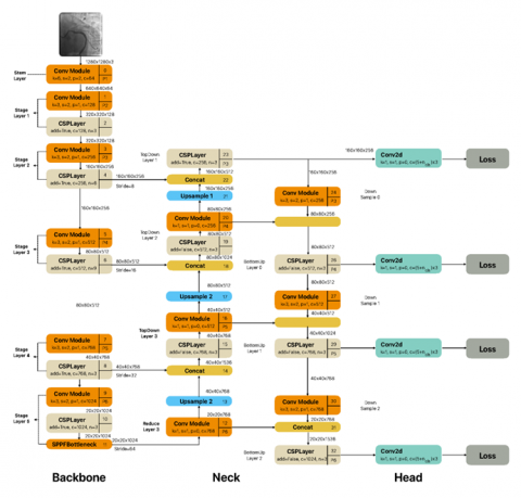
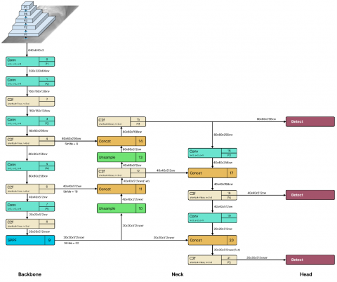
YOLO v5, on the other hand, produces extremely good results in tiny models due to the enhancements implemented. Although the main network techniques in YOLO v3 and YOLO v5 were similar, they both focused on recognizing objects of varying sizes at three different scales. YOLO v7 was quicker and more precise than V5 [23]. YOLO v8 was released in January 2023 by Ultralytics, the company that created YOLO v5. While it has a similar core structure to YOLO v5, there have been several changes to the CSPLayer (C2f module). This module improves detection accuracy by integrating high-level characteristics and contextual information [25]. It comes in five scale versions: YOLO v8n (nano), YOLO v8s (small), YOLOv8m (medium), YOLO v8l (large), and YOLO v8x (extra-large), all supporting several image processing tasks, including object identification, segmentation, posture estimation, tracking, and classification [39]. Figures 7-9 depict Yolo v5, v7 and v8 architectures employed in this study, respectively.
Figure 7. YOLO v5 architecture [25, 36]
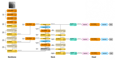
Figure 8. YOLO v7 architecture [25, 36]
Figure 9. YOLO v8 architecture [25, 36]
In this study, YOLOv5, YOLOv7, and YOLOv8 were selected due to their widespread use, high accuracy, and proven real-time detection capabilities in recent medical imaging applications [40]. YOLOv5 is known for its stability and compatibility with a variety of deployment environments. YOLOv7 offers enhanced accuracy and model optimization, while YOLOv8, the latest version, introduces improved backbone architecture and anchor-free detection. Earlier versions (YOLOv3, YOLOv4) were excluded due to their relatively outdated performance benchmarks and lack of support for recent training frameworks. Similarly, although EfficientDet and RetinaNet are strong contenders, YOLO models were prioritized for their superior inference speed, making them more suitable for real-time clinical applications.
In deep learning research, performance metrics play a crucial role in gauging and refining how well models work. They help researchers see how accurately a model predicts outcomes and guide improvements, especially for tasks like object detection and classification. For object detection and classification tasks, these include mean average precision (MAP), precision, recall, and F1 score [41, 42], which offer insight into both the precision and reliability of the model’s detections across a variety of conditions and dataset complexities.
The MAP measure used in object detection is a crucial parameter for determining the model’s accuracy level. For each cutoff threshold, precision and recall data are computed to be used in creating a precision-recall curve. MAP, as the average of the area under this curve, gives a summary of the model’s performance at different cutoff levels [43]. A higher MAP value indicates that the model performs better in object identification. For object detection, the MAP value is used to determine at which cutoff criteria the model performs better or worse, allowing for an objective evaluation of the model’s performance.
As an example, Figure 10 depicts two distinct clusters that indicate the grouping of each pixel in the detected and known images by counting them one by one [44] This visualization provides insights into the actual outcomes in comparison to the predicted responses, enhancing the understanding of the models’ detection performance [45].
Figure 10. Evaluation of region forecast performance [44]
Confusion Matrix is a fundamental tool for evaluating the performance of classification models, providing four key values that provide insights into the model’s predictive capabilities.
● True Positive (TP) indicates the number of samples that are correctly predicted as positive when they are indeed positive.
● True Negative (TN) represents the samples that are accurately predicted as negative when they are actually negative.
● False Positive (FP) reflects the number of samples that are incorrectly predicted as positive despite being negative.
● False Negative (FN) refers to samples that are inaccurately predicted as negative when they are truly positive [46].
These values serve as the basis for calculating several key performance metrics, including accuracy, precision, recall, and F1 score.
Accuracy is a primary performance metric utilized in classification tasks and is calculated as the ratio of correct predictions (both TP and TN) to total number of samples (Eq. (1)). In other words, it represents the proportion of correctly identified samples within the entire dataset.
Accuracy $=\frac{T N+T P}{T N+F N+F P+T P}$ (1)
This measure serves as an essential indicator of the model’s overall effectiveness, providing a straightforward assessment of its classification capabilities. However, it alone may not be sufficient, especially in cases of class imbalance.
Precision is an additional performance parameter utilized in classification tasks to measure the proportion of true positive predictions relative to the total positive predictions made by the model (Eq. (2)) [47]. In other words, it indicates how effectively the model identifies positive cases without misclassifying negatives as positives. A higher precision value indicates a more reliable model when it comes to identifying positive instances, thus minimizing the risk of incorrectly labeling negative cases as positive.
Precision $=\frac{T P}{F P+T P}$ (2)
Recall, also known as sensitivity, complements precision by measuring the ratio of true positives to the actual positive cases. It is the ratio of accurately identified positive cases to the actual number of positive cases (Eq. (3)). In other words, it measures the model’s ability to recognize all relevant instances within the dataset. A higher recall value indicates that the model is adept at detecting positive cases, making it particularly valuable in applications where missing a positive instance is critical.
Recall $=\frac{T P}{F N+T P}$ (3)
A common challenge in model evaluation is the trade-off between precision and recall; improving one often leads to a decrease in the other. While precision focuses on reducing false positives, recall aims to capture as many true positives as possible [47]. Therefore, adjusting the cutoff levels becomes essential to find a balance between precision and recall, optimizing overall model performance.
F1 Score serves as the harmonic average of the precision and recall values, providing a single score that reflects both accuracy and recall. It is particularly useful when dealing with imbalanced datasets, as it emphasizes the importance of both identifying positive instances correctly and minimizing false positives (Eq. (4)). By integrating both precision and recall, the F1 score offers a comprehensive assessment of a model’s performance, making it a valuable tool for model evaluation.
$\mathrm{F} 1=\frac{2 * \text { Precision } * \text { Recall }}{\text { Precision }+ \text { Recall }}$ (4)
Loss function is a crucial parameter in evaluating a model’s performance, serving as a measure of error and success. Its primary role is to quantify the deviation of predictions from the true values, providing a numerical indication of how well the model performs. Ideally, a well-optimized architecture will yield a loss function value close to zero, indicating accurate predictions. Conversely, if the model’s predictions are significantly off, the loss function value approaches one, reflecting poor performance. Consequently, minimizing the loss function becomes a key objective during model training, guiding the optimization process to improve accuracy. This metric not only assesses the effectiveness of the model but also plays a vital role in updating the model's parameters to enhance learning [48].
In this study, we evaluated the performance of YOLO v5, v7, and v8 on four distinct test sets derived from the initial dataset. Each test set was trained to ensure a comprehensive assessment of the models’ capabilities. The training phase involved utilizing the training datasets to optimize the models, followed by rigorous evaluation using the respective test datasets. Each model underwent training for a total of 100 epochs, a process designed to refine their learning and enhance performance. This structured approach enabled a thorough analysis of each model’s effectiveness in object detection, providing valuable insights into their strengths and limitations across the various datasets. The subsequent sections will detail the findings from these evaluations, highlighting the models’ accuracy, precision, and overall effectiveness in detecting the specified targets. The experimental results in this study were achieved using the computational resources of UHeM Altay [49] cluster system with applications written in Python programming language.
Table 1 outlines the hyperparameters employed during the training of the YOLO models. Hyperparameters are crucial for determining the behavior and effectiveness of the learning process. Each parameter is carefully selected to optimize the models’ performances.
Table 1. Hyper parameters
|
Parameter |
Value |
|
Image Size |
512×512 |
|
Batch |
16 |
|
Epoch |
100 |
|
Base Weights |
yolov5 x.pt yolov7.pt yolov8 x.pt |
The selection of hyperparameters such as batch size and the number of epochs is crucial in optimizing model performance and ensuring efficient training. A batch size of 16 was chosen based on the trade-off between computational efficiency and model stability. Larger batch sizes can speed up the training process but may lead to less accurate gradient estimates, potentially hindering convergence. Conversely, smaller batch sizes provide more precise gradient updates but can significantly increase training time. A moderate batch size of 16 helps balance these aspects, promoting stable learning while managing memory constraints [27, 28]. The number of epochs, set at 100, was determined through preliminary experiments, where increasing the epochs beyond this value showed diminishing returns in terms of performance improvement. This indicates that 100 epochs were sufficient for the model to learn the underlying patterns in the data without risking overfitting. By fine-tuning these hyperparameters, we aimed to achieve a balance between training efficiency and model accuracy, thereby optimizing the learning process for the YOLO models employed in this study.
Image Size (512×512): This parameter indicates the dimensions of the input images processed by the models. By choosing a size of 512×512 pixels, we ensure that the images retain enough detail for effective feature extraction while maintaining a balance between computational efficiency and memory usage. This size is commonly used in object detection tasks, as it allows the model to capture essential features while avoiding excessive resource consumption.
Batch Size (16): The batch size refers to the number of training samples processed before the model’s weights are updated. A batch size of 16 was selected to promote stability during training while managing memory constraints. This size helps to smooth the gradient estimates during the backpropagation process, allowing for more reliable updates to the model's parameters.
Epochs (100): An epoch represents one complete pass through the entire training dataset. Training for 100 epochs was found to be sufficient for allowing the models to learn the underlying patterns in the data. This extended training duration provides the models with ample opportunity to refine their weights, potentially leading to improved performance on unseen data.
Base Weights: The base weights utilized for each YOLO version were specifically chosen to leverage the pre-trained knowledge obtained from prior tasks. The selected weights, such as yolov5x.pt, yolov7.pt, and yolov8x.pt, facilitate a quicker convergence during training. By initializing the models with these pre-trained weights, we aim to enhance the detection capabilities of the models on the angiographic dataset, as they can build on previously learned features.
To enhance generalization and reduce overfitting, data augmentation was applied during training. The YOLO training pipeline included standard augmentation techniques such as horizontal flipping, random rotations within ±10°, brightness and contrast adjustments, and mosaic augmentation. These techniques helped simulate variations in imaging conditions and anatomical orientation, thereby improving the robustness of the detection models.
Table 2 presents the training times for each YOLO model across the four datasets, highlighting the computational demands associated with training each configuration. The training durations reported reflect the total time taken for each model to complete the training process on each dataset.
Table 2. Training times for the models
|
Model |
Data Set |
Training Time |
|
YOLO v5 |
Dataset 1 |
2:51:31 |
|
Dataset 2 |
2:52:20 |
|
|
Dataset 3 |
2:49:48 |
|
|
Dataset 4 |
2:47:24 |
|
|
YOLO v7 |
Dataset 1 |
8:42:45 |
|
Dataset 2 |
9:16:52 |
|
|
Dataset 3 |
9:04:34 |
|
|
Dataset 4 |
9:08:28 |
|
|
YOLO v8 |
Dataset 1 |
4:07:12 |
|
Dataset 2 |
4:07:02 |
|
|
Dataset 3 |
4:07:10 |
|
|
Dataset 4 |
4:05:47 |
As seen, YOLO v5 exhibited the shortest training times, indicating its efficiency in processing the data. This rapid training capability is advantageous in practical applications where timely results are critical, especially in clinical settings that rely on swift decision-making. In contrast, YOLO v7 demonstrated significantly longer training durations, with times extending beyond 8 hours for the initial dataset and even longer for subsequent datasets. Such prolonged training periods may suggest a more complex model architecture or difficulties in convergence, potentially stemming from the dataset’s intricacies or the model’s inherent characteristics. YOLO v8, while not as swift as YOLO v5, completed training in approximately 4 hours, indicating a balanced approach in terms of efficiency and model capability. This intermediate training time underscores YOLO v8’s ability to manage complexity while still providing reasonable training durations.
To assess real-time applicability, inference speed was measured on a single NVIDIA A100 GPU (40GB). YOLOv5 achieved an average of 75 frames per second (FPS), YOLOv8 reached 65 FPS, and YOLOv7 recorded 45 FPS for 512x512 image input. These results affirm YOLOv5’s suitability for real-time clinical environments, where fast decision-making is crucial. GPU memory usage was also evaluated, with YOLOv5 requiring the least memory (~4.8GB) and YOLOv7 the most (~8.2GB). These measurements underscore the trade-offs between model complexity and deployment feasibility in resource-constrained hospital settings.
Figure 11 illustrates the evolution of loss values throughout the training epochs for each YOLO model, offering a visual representation of the models’ learning processes. The figure displays the trajectories of loss values for each model, providing insights into their respective training dynamics. A consistent decline in loss values, particularly for YOLO v5 and YOLO v8, suggests effective optimization and learning throughout the training epochs. This trend indicates that these models successfully adjusted their weights in response to the training data, thereby enhancing their ability to generalize to new, unseen data. Conversely, fluctuations or less consistent patterns in the loss values for YOLO v7 may indicate potential challenges during training. Such irregularities can be attributed to several factors, including the model’s complexity, learning rate adjustments, or specific dataset characteristics that may hinder convergence.
Figure 11. Loss changes during training
Figure 11 illustrates the changes in loss values over the training epochs for YOLO v5, v7, and v8. The loss values for YOLO v5 and YOLO v8 show a consistent decrease, indicating effective learning and optimization throughout the training process. YOLO v5 achieved lower final loss values compared to the other models, suggesting a quicker convergence and a better fit to the training data. In contrast, YOLO v7 exhibited more fluctuation in its loss values, potentially due to challenges in optimizing the model parameters effectively. This instability may be attributed to the complexity of the model architecture or sensitivity to specific features in the datasets, highlighting the need for further fine-tuning of hyperparameters to achieve stable learning.
After the training, model performances were evaluated using test images that were not included in the training process in the datasets. This evaluation was critical to ensure that the models could generalize their learning to new, unseen data effectively. Table 3 summarizes the performance metrics obtained from evaluating each YOLO model against the test images. The table provides key metrics such as F1 Score, F1 Score Confidence, Precision, Recall, Mean Average Precision (mAP) at an Intersection over Union (IoU) threshold of 0.5, and Accuracy. These metrics collectively offer a comprehensive assessment of the models’ detection capabilities, emphasizing not only their accuracy in identifying blockages but also their reliability across different datasets.
Table 3. Test results
|
Model |
Dataset |
F1 Score |
F1 Score Confidence |
Precision |
Recall |
MAP@0.5 |
Accuracy |
|
YOLO v5 |
Dataset 1 |
0.98 |
0.538 |
0.897 |
0.99 |
0.982 |
0.98 |
|
Dataset 2 |
0.97 |
0.377 |
0.877 |
0.98 |
0.976 |
0.98 |
|
|
Dataset 3 |
0.98 |
0.411 |
0.904 |
0.99 |
0.980 |
0.98 |
|
|
Dataset 4 |
0.38 |
0.032 |
0.902 |
0.31 |
0.323 |
0.24 |
|
|
YOLO v7 |
Dataset 1 |
0.48 |
0.208 |
0.902 |
0.90 |
0.426 |
0.38 |
|
Dataset 2 |
0.62 |
0.255 |
0.856 |
0.94 |
0.615 |
0.57 |
|
|
Dataset 3 |
0.46 |
0.183 |
0.837 |
0.90 |
0.418 |
0.34 |
|
|
Dataset 4 |
0.23 |
0.204 |
0.733 |
0.60 |
0.149 |
0.18 |
|
|
YOLO v8 |
Dataset 1 |
0.98 |
0.588 |
0.857 |
0.98 |
0.984 |
0.98 |
|
Dataset 2 |
0.97 |
0.521 |
0.869 |
0.98 |
0.980 |
0.98 |
|
|
Dataset 3 |
0.97 |
0.454 |
0.818 |
0.98 |
0.985 |
0.98 |
|
|
Dataset 4 |
0.35 |
0.027 |
0.855 |
0.26 |
0.401 |
0.23 |
According to the Table 3, YOLO v5 performed best overall, particularly in Dataset 1, 2, and 3, achieving F1 Scores above 0.97, in addition to offering high precision. YOLO v7 had the lowest scores across all datasets, indicating potential issues in model performance, especially in Dataset 4. YOLO v8 showed strong performance comparable to YOLO v5, maintaining high F1 Scores and precision across Datasets 1, 2, and 3, but struggled with Dataset 4. The high F1 scores observed in YOLO v5 and YOLO v8 across the initial three datasets indicate their robustness in detecting vascular occlusions, reflecting their ability to maintain a balance between precision and recall.
However, the significant drop in performance for Dataset 4, particularly for YOLO v5, prompts a deeper investigation into this dataset’s unique characteristics that may have contributed to this variance. Analyzing the discrepancies in performance across datasets provides valuable insights into potential model limitations and areas for improvement.
Figure 12 presents sample results from all datasets, showcasing the outputs generated by the YOLO models in the context of vascular occlusion detection. Each entry in the figure includes a representative example of the model’s predictions, illustrating how accurately the models identified and localized the specified targets within the angiographic images. The samples are selected to highlight each model’s performance across different datasets, demonstrating their ability to generalize their learning the images that are not used for training. This figure not only serves to visualize the effectiveness of the detection algorithms but also provides a comparative perspective on how each model performs in identifying occlusions under varying conditions and complexities present in the datasets. By examining these results, we gain insights into the models’ strengths in accurately recognizing vascular blockages, as well as any potential limitations in their detection capabilities.
Figure 12. YOLO Models’ sample predictions for vascular occlusion detection across the datasets
Figure 12 displays representative samples of the predictions made by YOLO v5, v7, and v8 across different datasets. The visual comparisons highlight the models' abilities to accurately identify and localize areas of vascular occlusion. YOLO v5 and YOLO v8 consistently detected stenotic regions with high precision in most samples, particularly in Datasets 1, 2, and 3. However, the performance variability of YOLO v7, especially in Dataset 4, suggests limitations in handling more complex or less distinct features present in certain angiographic images. These results emphasize the differences in model generalization capabilities and the impact of dataset characteristics on detection performance.
In this study, YOLO v5 demonstrated superior performance across Datasets 1, 2, and 3, achieving F1 scores consistently above 0.97, along with high precision and recall values. These findings underscore YOLO v5’s effectiveness in accurately detecting stenotic regions, suggesting its potential suitability for clinical applications requiring high accuracy and reliability.
In contrast, YOLO v7 displayed notably lower performances across all datasets, particularly under the conditions presented by Dataset 4. The reduced accuracy and recall values for YOLO v7 suggest potential limitations in handling complex groupings within angiographic images, pointing to a need for further model optimization when addressing more intricate image classifications.
Notably, YOLO v8 yielded competitive performance with YOLO v5, achieving similar F1 scores and precision metrics across Datasets 1, 2, and 3. However, both models exhibited challenges in Dataset 4, likely due to the unique and complex structure of this dataset, which may require further adaptation of YOLO architectures for optimal performance.
This study evaluated the performance of YOLO v5, YOLO v7, and YOLO v8 in detecting vascular occlusions from angiographic images. Overall, YOLO v5 exhibited exceptional performance across the datasets, particularly in scenarios characterized by random assignments and ID-based groupings. Its strong precision and recall metrics underscore its efficacy in recognizing angiographic features, making it highly suitable for clinical applications, particularly in real-time settings where accurate detection is crucial.
Similarly, YOLO v8 demonstrated robust capabilities across the datasets, showcasing its potential utility in clinical environments. In contrast, YOLO v7 consistently underperformed, particularly in more complex grouping configurations, indicating possible limitations in its architecture. Notably, Dataset 4 presented significant challenges for all models, highlighting the necessity for further investigation into the models' capabilities when subjected to stringent classification criteria.
The consistently high accuracy and precision metrics of YOLO v5 and YOLO v8 across three of the four datasets affirm these models' capabilities in identifying stenotic areas within angiographic images. These results are particularly relevant in clinical scenarios such as the assessment of coronary artery stenosis, where the ability to reliably detect occlusions can support rapid diagnosis and assist cardiologists in making timely treatment decisions. The integration of such advanced detection algorithms into clinical workflows could enhance diagnostic processes and improve patient outcomes.
In contrast, YOLO v7’s lower performance metrics across all datasets, especially in Dataset 4, suggest challenges in identifying intricate details within angiographic images. The noticeably lower performance of YOLO v7 across all datasets, particularly in Dataset 4, can be attributed to several factors related to the model’s architecture and adaptation capabilities. One possible reason for this underperformance is the model’s sensitivity to dataset diversity. Unlike YOLO v5 and YOLO v8, which incorporate more advanced features for generalization, YOLO v7 may struggle to effectively adapt its weights to varying data characteristics, such as differences in image resolution, contrast, and occlusion complexity. This limitation suggests that YOLO v7’s architecture may lack the robustness needed to handle highly heterogeneous datasets, leading to inconsistencies in detection accuracy. Furthermore, the design of YOLO v7, while optimized for speed, may sacrifice certain aspects of feature extraction that are crucial for detecting fine-grained details in complex medical images.
It is worth noting that the dataset employed in this study was curated to include only angiographic frames containing at least one annotated stenotic region. As such, every image presented a positive detection target, thereby reducing the risk of extreme class imbalance often observed in pixel-level classification tasks. Moreover, the YOLO architecture handles object detection through region-level predictions with built-in confidence and objectless scoring mechanisms, which inherently mitigate the effects of background-to-object imbalance. Therefore, additional strategies such as Focal Loss or weighted sampling were not deemed necessary for this application.
Dataset 4 posed significant challenges for all models, with a marked decrease in performance metrics, especially for YOLO v7. This dataset likely contained more complex and less distinct stenotic features, which are harder to identify due to variations in contrast, vessel overlap, and noise. The decline in performance suggests that the models, especially YOLO v7, struggled with the intricate structures present in these images, indicating a potential weakness in handling high variability and subtle visual patterns. These findings highlight the importance of dataset characteristics in evaluating model performance and underscore the need for further enhancements in YOLO v7’s feature extraction and adaptation mechanisms to improve its reliability in complex medical imaging tasks.
Although the study analyzes individual frames, these images are extracted from full coronary angiographic sequences and thus inherently reflect various phases of contrast agent flow. While we did not explicitly model temporal dynamics across consecutive frames, the spatial features captured in these images correspond to meaningful stages in the vascular filling process. Future work will aim to integrate time-sequential data or video-based deep learning approaches to better leverage temporal vessel behavior and support functional assessment of stenosis.
These limitations may stem from inherent architectural constraints that hinder the model’s adaptability to complex patterns, as evidenced in highly structured image groupings. Future work may benefit from modifying YOLO v7’s structure or exploring alternative configurations better suited for medical imaging applications.
The comparative analysis of Dataset 4 underscores the significant impact of dataset structure on model performance, as all YOLO versions encountered difficulties with this grouping. This observation emphasizes the importance of dataset characteristics when training deep learning models for complex clinical tasks. Adapting YOLO architectures to effectively manage the variability within detailed angiographic data may enhance their diagnostic reliability and clinical applicability.
From a clinical perspective, both false positives and false negatives present significant concerns. False negatives may result in missed diagnoses of critical stenotic lesions, potentially leading to untreated ischemia or myocardial infarction. Conversely, false positives could prompt unnecessary invasive procedures. In this study, a confidence threshold of 0.5 was applied uniformly across models; however, optimizing this value based on precision-recall trade-offs could help reduce diagnostic errors. Future work will focus on threshold tuning and post-processing rules tailored for high-risk clinical applications to ensure patient safety and diagnostic reliability.
In conclusion, while YOLO v5 and YOLO v8 show promising results for angiographic image classification, further research is essential to address the challenges observed in complex datasets and to optimize YOLO v7 for enhanced performance in clinical scenarios. Future research could focus on integrating additional image modalities, such as 3D angiography or multi-spectral imaging, to further enhance detection accuracy and develop a more comprehensive diagnostic tool for clinical use. Additionally, exploring ensemble learning techniques or combining YOLO models with other advanced architectures could provide more robust solutions for detecting subtle vascular abnormalities, ultimately improving the reliability and applicability of these methods in real-world clinical settings.
This paper was supported by National Center for High Performance Computing of Turkey (UHeM) (Grant No.: 016482023).
[1] Le, A., Peng, H., Golinsky, D., Di Scipio, M., Lali, R., Paré, G. (2024). What causes premature coronary artery disease? Current Atherosclerosis Reports, 26(6): 189-203. https://doi.org/10.1007/s11883-024-01200-y
[2] Malakar, A.K., Choudhury, D., Halder, B., Paul, P., Uddin, A., Chakraborty, S. (2019). A review on coronary artery disease, its risk factors, and therapeutics. Journal of Cellular Physiology, 234(10): 16812-16823. https://doi.org/10.1002/jcp.28350
[3] Townsend, N., Kazakiewicz, D., Lucy Wright, F., Timmis, A., Huculeci, R., Torbica, A., Gale, C.P., Achenbach, S., Weidinger, F., Vardas, P. (2022). Epidemiology of cardiovascular disease in Europe. Nature Reviews Cardiology, 19(2): 133-143. https://doi.org/10.1038/s41569-021-00607-3
[4] Khaltaev, N., Axelrod, S. (2022). Countrywide cardiovascular disease prevention and control in 49 countries with different socio-economic status. Chronic Diseases and Translational Medicine, 8(4): 296-304. https://doi.org/10.1002/cdt3.34
[5] Priyanka, N., Kumar, P.R. (2017). Usage of data mining techniques in predicting the heart diseases-Naïve Bayes & decision tree. In 2017 International Conference on Circuit, Power and Computing Technologies (ICCPCT), Kollam, India, pp. 1-7. https://doi.org/10.1109/ICCPCT.2017.8074215
[6] Matta, M., Harb, S.C., Cremer, P., Hachamovitch, R., Ayoub, C. (2021). Stress testing and noninvasive coronary imaging: What’s the best test for my patient? Cleveland Clinic Journal of Medicine, 88(9): 502-515. https://doi.org/10.3949/ccjm.88a.20068
[7] Tesche, C., De Cecco, C.N., Albrecht, M.H., Duguay, T. M., Bayer, R.R., Litwin, S.E., Steinberg, D.H., Schoepf, U.J. (2017). Coronary CT angiography-derived fractional flow reserve. Radiology, 285(1): 17-33. https://doi.org/10.1148/radiol.2017162641
[8] Han, D., Liu, J., Sun, Z., Cui, Y., He, Y., Yang, Z. (2020). Deep learning analysis in coronary computed tomographic angiography imaging for the assessment of patients with coronary artery stenosis. Computer Methods and Programs in Biomedicine, 196: 105651. https://doi.org/10.1016/j.cmpb.2020.105651
[9] Danilov, V.V., Klyshnikov, K.Y., Gerget, O.M., Kutikhin, A.G., Ganyukov, V.I., Frangi, A.F., Ovcharenko, E.A. (2021). Real-time coronary artery stenosis detection based on modern neural networks. Scientific Reports, 11(1): 7582. https://doi.org/10.1038/s41598-021-87174-2
[10] El Sherbini, A., Rosenson, R.S., Al Rifai, M., Virk, H.U.H., Wang, Z., Virani, S., Glicksberg, B.S., Lavie, C.J., Krittanawong, C. (2024). Artificial intelligence in preventive cardiology. Progress in Cardiovascular Diseases, 84: 76-89. https://doi.org/10.1016/j.pcad.2024.03.002
[11] Wang, X., Zhu, H. (2024). Artificial intelligence in image-based cardiovascular disease analysis: A comprehensive survey and future outlook. arXiv Preprint arXiv: 2402.03394. https://doi.org/10.48550/arXiv.2402.03394
[12] Cai, L., Gao, J., Zhao, D. (2020). A review of the application of deep learning in medical image classification and segmentation. Annals of Translational Medicine, 8(11): 713. https://doi.org/10.21037/atm.2020.02.44
[13] Zhang, X., Zhang, B., Zhang, F. (2024). Stenosis detection and quantification of coronary artery using machine learning and deep learning. Angiology, 75(5): 405-416. https://doi.org/10.1177/00033197231187063
[14] Sameh, S., Azim, M.A., AbdelRaouf, A. (2017). Narrowed coronary artery detection and classification using angiographic scans. In 2017 12th International Conference on Computer Engineering and Systems (ICCES), Cairo, Egypt, pp. 73-79. https://doi.org/10.1109/ICCES.2017.8275280
[15] Wan, T., Feng, H., Tong, C., Li, D., Qin, Z. (2018). Automated identification and grading of coronary artery stenoses with X-ray angiography. Computer Methods and Programs in Biomedicine, 167: 13-22. https://doi.org/10.1016/j.cmpb.2018.10.013
[16] Antczak, K., Liberadzki, Ł. (2018). Stenosis detection with deep convolutional neural networks. MATEC Web of Conferences, 210: 04001. https://doi.org/10.1051/matecconf/201821004001
[17] Wu, W., Zhang, J., Xie, H., Zhao, Y., Zhang, S., Gu, L. (2020). Automatic detection of coronary artery stenosis by convolutional neural network with temporal constraint. Computers in Biology and Medicine, 118: 103657. https://doi.org/10.1016/j.compbiomed.2020.103657
[18] Danilov, V.V., Gerget, O.M., Klyshnikov, K.Y., Frangi, A.F., Ovcharenko, E.A. (2021). Analysis of deep neural networks for detection of coronary artery stenosis. Programming and Computer Software, 47(3): 153-160. https://doi.org/10.1134/S0361768821030038
[19] Pang, K., Ai, D., Fang, H., Fan, J., Song, H., Yang, J. (2021). Stenosis-DetNet: Sequence consistency-based stenosis detection for X-ray coronary angiography. Computerized Medical Imaging and Graphics, 89: 101900. https://doi.org/10.1016/j.compmedimag.2021.101900
[20] Ovalle-Magallanes, E., Avina-Cervantes, J.G., Cruz-Aceves, I., Ruiz-Pinales, J. (2022). Improving convolutional neural network learning based on a hierarchical bezier generative model for stenosis detection in X-ray images. Computer Methods and Programs in Biomedicine, 219: 106767. https://doi.org/10.1016/j.cmpb.2022.106767
[21] Ovalle-Magallanes, E., Avina-Cervantes, J.G., Cruz-Aceves, I., Ruiz-Pinales, J. (2022). LRSE-Net: Lightweight residual squeeze-and-excitation network for stenosis detection in X-ray coronary angiography. Electronics, 11(21): 3570. https://doi.org/10.3390/electronics11213570
[22] Han, T., Ai, D., Li, X., Fan, J., Song, H., Wang, Y., Yang, J. (2023). Coronary artery stenosis detection via proposal-shifted spatial-temporal transformer in X-ray angiography. Computers in Biology and Medicine, 153: 106546. https://doi.org/10.1016/j.compbiomed.2023.106546
[23] Jiang, P., Ergu, D., Liu, F., Cai, Y., Ma, B. (2022). A review of YOLO algorithm developments. Procedia Computer Science, 199: 1066-1073. https://doi.org/10.1016/j.procs.2022.01.135
[24] Redmon, J., Divvala, S., Girshick, R., Farhadi, A. (2016). You only look once: Unified, real-time object detection. In Proceedings of the IEEE Conference on Computer Vision and Pattern Recognition, pp. 779-788. https://doi.org/10.48550/arXiv.1506.02640
[25] Hussain, M. (2023). YOLO-v1 to YOLO-v8, the rise of YOLO and its complementary nature toward digital manufacturing and industrial defect detection. Machines, 11(7): 677. https://doi.org/10.3390/machines11070677
[26] Farhadi, A., Redmon, J. (2018). Yolov3: An incremental improvement. In Computer Vision and Pattern Recognition, Berlin/Heidelberg, Germany: Springer, 1804: 1-6. https://doi.org/10.48550/arXiv.1804.02767
[27] Dutta, A., Zisserman, A. (2019). The VIA annotation software for images, audio and video. In Proceedings of the 27th ACM International Conference on Multimedia, pp. 2276-2279. https://doi.org/10.1145/3343031.3350535
[28] Matsuo, Y., LeCun, Y., Sahani, M., Precup, D., Silver, D., Sugiyama, M., Uchibe, E., Morimoto, J. (2022). Deep learning, reinforcement learning, and world models. Neural Networks, 152: 267-275. https://doi.org/10.1016/j.neunet.2022.03.037
[29] Taşova, O. (2011). Yapay sinir ağlari ile yüz tanima. Master's Thesis, Dokuz Eylul Universitesi (Turkey), DEÜ Fen Bilimleri Enstitüsü.
[30] Rusk, N. (2016). Deep learning. Nature Methods, 13(1): 35. https://doi.org/10.1038/nmeth.3707
[31] Shinde, P.P., Shah, S. (2018). A review of machine learning and deep learning applications. In 2018 Fourth International Conference on Computing Communication Control and Automation (ICCUBEA), Pune, India, pp. 1-6. https://doi.org/10.1109/ICCUBEA.2018.8697857
[32] Huang, R., Pedoeem, J., Chen, C. (2018). YOLO-LITE: A real-time object detection algorithm optimized for non-GPU computers. In 2018 IEEE International Conference on Big Data (Big Data), Seattle, USA, pp. 2503-2510. https://doi.org/10.1109/BigData.2018.8621865
[33] Wu, J. (2017). Introduction to convolutional neural networks. National Key Lab for Novel Software Technology, Nanjing University, China, 5(23): 495.
[34] Chua, L.O., Roska, T. (1993). The CNN paradigm. IEEE Transactions on Circuits and Systems I: Fundamental Theory and Applications, 40(3): 147-156. https://doi.org/10.1109/81.222795
[35] LeCun, Y., Bottou, L., Bengio, Y., Haffner, P. (2002). Gradient-based learning applied to document recognition. Proceedings of the IEEE, 86(11): 2278-2324. https://doi.org/10.1109/5.726791
[36] Liao, J., Jiang, S., Chen, M., Sun, C. (2025). SAM-YOLO: An improved small object detection model for vehicle detection. The European Journal on Artificial Intelligence, 38(3): 279-295. https://doi.org/10.1177/30504554251319452
[37] Tan, M., Pang, R., Le, Q.V. (2020). Efficientdet: Scalable and efficient object detection. In Proceedings of the IEEE/CVF Conference on Computer Vision and Pattern Recognition, pp. 10781-10790. https://doi.org/10.48550/arXiv.1911.09070
[38] Dodia, A., Kumar, S. (2023). A comparison of YOLO based vehicle detection algorithms. In 2023 International Conference on Artificial Intelligence and Applications (ICAIA) Alliance Technology Conference (ATCON-1), Bangalore, India, pp. 1-6. https://doi.org/10.1109/ICAIA57370.2023.10169773
[39] Kim, J.H., Kim, N., Won, C.S. (2023). High-speed drone detection based on YOLO-v8. In ICASSP 2023-2023 IEEE International Conference on Acoustics, Speech and Signal Processing (ICASSP), Rhodes Island, Greece, pp. 1-2. https://doi.org/10.1109/ICASSP49357.2023.10095516
[40] Bochkovskiy, A., Wang, C.Y., Liao, H.Y.M. (2020). Yolov4: Optimal speed and accuracy of object detection. arXiv Preprint arXiv: 2004.10934. https://doi.org/10.48550/arXiv.2004.10934
[41] Susmaga, R. (2004). Confusion matrix visualization. In Intelligent Information Processing and Web Mining: Proceedings of The International IIS: IIPWM ‘04 Conference Held in Zakopane, Poland, Berlin, Heidelberg: Springer Berlin Heidelberg, pp. 107-116. https://doi.org/10.1007/978-3-540-39985-8_12
[42] Tello-Mijares, S., Woo, F., Flores, F. (2019). Breast cancer identification via thermography image segmentation with a gradient vector flow and a convolutional neural network. Journal of Healthcare Engineering, 2019(1): 9807619. https://doi.org/10.1155/2019/9807619
[43] Revaud, J., Almazán, J., Rezende, R.S., Souza, C.R.D. (2019). Learning with average precision: Training image retrieval with a listwise loss. In Proceedings of the IEEE/CVF International Conference on Computer Vision, Seoul, Korea (South), pp. 5107-5116. https://doi.org/10.1109/ICCV.2019.00521
[44] Li, X., Wang, Z., He, T., Gong, H., Duan, Z., Wei, Y., Gong, Y. (2017). Study on radial sheet beam electron optical system for miniature low-voltage traveling-wave tube. IEEE Transactions on Electron Devices, 64(8): 3405-3412. https://doi.org/10.1109/TED.2017.2711616
[45] Kuznetsova, A.A. (2021). Statistical precision-recall curves for object detection algorithms performance measurement. In Cyber-Physical Systems: Modelling and Intelligent Control. Springer, Cham, 335-348. https://doi.org/10.1007/978-3-030-66077-2_27
[46] Visa, S., Ramsay, B., Ralescu, A.L., Van Der Knaap, E. (2011). Confusion matrix-based feature selection. Maics, 710(1): 120-127.
[47] Goutte, C., Gaussier, E. (2005). A probabilistic interpretation of precision, recall and F-score, with implication for evaluation. In European Conference on Information Retrieval. Berlin, Heidelberg: Springer Berlin Heidelberg, pp. 345-359. https://doi.org/10.1007/978-3-540-31865-1_25
[48] Wu, L., Zhu, Z. (2017). Towards understanding generalization of deep learning: Perspective of loss landscapes. arXiv Preprint arXiv: 1706.10239. https://doi.org/10.48550/arXiv.1706.10239
[49] UHeM. The National Center for High Performance Computing (UHeM). https://en.uhem.itu.edu.tr/donanim.html, accessed on 2024.