Kalaimathi Bathirappan*![]() | Jayanthy Soundararajan
| Jayanthy Soundararajan![]()
© 2024 The authors. This article is published by IIETA and is licensed under the CC BY 4.0 license (http://creativecommons.org/licenses/by/4.0/).
OPEN ACCESS
License plate detection from moving vehicles is useful in authenticating owners, detecting vehicle misbehaviors, etc. Roadside video outputs are analyzed using computer vision-based algorithms/ methods to improve the detection precision. This article thus introduces a Boundary Filtering Method (BFM) using Conditional Neural Learning (CNL). In this method, the conventional neural network with filtering conditions is used to identify the license plate boundary. The congruent textural features are filtered based on trained inputs from datasets. The similar boundary indices identified in the training images are used to shape the license plate region from the frame inputs. The conditions of maximum similarity and boundary displacement connectivity are verified throughout the training process until maximum precision is reached. The condition-failing features are filtered to reduce the false positives between different frame orientations. The proposed method is verified using accuracy, precision, similarity index, false positives, and time metrics. The proposed method improves precision by 9.57%and reduces false positives and analysis time by 10.43% and 6.28% respectively for the boundaries identified.
boundary detection, feature extraction, license plate detection, neural network, similarity index
In computer vision and security, the identification of vehicle license plates from surveillance footage is an essential application. First, surveillance footage is extracted into frames [1]. To handle privacy problems and guarantee responsible technology usage, ethical and legal standards are crucial [2]. It is anticipated that further technology advancements will improve license plate border detecting systems' effectiveness and dependability, eventually enhancing general security and public safety [3].
The identification of automobile license plates from surveillance footage is greatly aided by deep learning [4]. Relying on sophisticated neural network designs, including region-based models or convolutional neural networks (CNNs), makes it possible to accurately identify license plates [5]. These algorithms get sophisticated characteristics from large datasets, which improves their capacity to identify plates in a variety of scenarios. Annotated datasets comprising pictures of cars and the license plates that go with them are used for training [6]. By identifying license plate areas on its own, the deep learning algorithm eliminates the requirement for human feature engineering [7]. By using pre-trained models on huge picture datasets, transfer learning improves model efficiency even further. The ongoing progress in deep learning methodologies aids in the enhancement of license plate recognition systems, rendering them more resilient and dependable in actual surveillance situations [8]. The major contributions of the article are:
The article’s organization is: Section 2 presents the discussion of different methods related to number plate detection with their pros and cons. In Section 3 the proposed boundary filtering method is discussed with suitable illustrations and explanations. Section 4 presents the experimental and comparative analysis results using real time images and metrics. Section 5 concludes the article with the findings, limitations, and future work.
Silva and Jung [9] introduced a flexible approach to automatic license plate recognition (ALPR). The primary objective of improve the effectiveness of current ALPR systems, particularly in scenarios involving oblique views and distorted angles of license plates. IWPOD-NET is designed to detect the corners of license plates, enabling the establishment of a front-parallel view. The method demonstrated superior ALPR performance across various analyzed datasets. Pan et al. [10] combined deep learning techniques for spotting and matching license plates in communicating vehicles. Their focus was on improving accuracy in detecting and recognizing license plates in Transportation IoT's V2V communication. The method enables the model to take advantage of the speed and accuracy of YOLOV3, as well as the exceptional detection capabilities of CRNN. The model scores high for license plate detection in terms of accuracy and precision.
Jia and Xie [11] proposed an efficient approach for license plate detection using deep neural networks across diverse scenarios. The primary goal is to improve the precision of identifying slanted or distorted license plates. The Deformation Planar Object Detection Network (DPOD-NET) network is specifically designed to correct perspective distortions in license plates. The method achieved higher performance with better accuracy and lower computational cost. Shi and Zhao [12] proposed a system for the identification of license plates using an improved YOLOv5 and GRU. A deep learning model addresses the accuracy and speed issues that are inherent in traditional approaches to license plate recognition. The channel attention mechanism enhances YOLOv5 with much better efficiency in extracting features. The model shows better stability and robustness in an environment that has been more complex than the ordinary environment.
Pan et al. [13] described an algorithm for the detection of license plates from remote surveillance. The suggested Automatic Super-Resolution License Plate Recognition network improves license plate recognition in surveillance, ensuring high-quality images are maintained. The detection model of LPs must be trained alone, and then its detection results will be used to successively train the subsequent modules. The method performs better with higher accuracy and improved image quality. Zhang et al. [14] introduced a real-time license plate recognition scheme using the CNN-CatBoost method. The method helps improve reality by overcoming poor visibility and irregular vehicle movements in real-time traffic scenarios. The method employs a CNN to deal with the visualization of license plates and refine identification using CatBoost. The combined model is even more accurate and efficient compared to other models that exist already.
Hamdi et al. [15] proposed a technique aiming to enhance license plate recognition accuracy through image improvement and super-resolution. The method specifically addresses challenges posed by blurry and low-quality license plate images. By effectively denoising and super-resolving, it ensures clearer identification, significantly improving accuracy in challenging scenarios. The method proves its effectiveness in real-world applications. Cao [16] introduced a method using convolutional neural networks (CNNs) to enhance license plate detection. The aim is to improve applications like law enforcement, toll collection, and parking management by deep learning. A huge labeled dataset is used to train the CNN-based model using supervised learning. The model is fine-tuned to obtain high accuracy in recognizing license plates, as is the demonstration on evaluations on both validation and new images.
Gautam et al. [17] presented an automatic license plate recognition model using deep learning. The approach uses deep learning-based Convolutional Neural Networks (CNNs) for tasks such as plate detection, rectification, and character recognition. CNNs locate corner points with the help of a mean squared error loss function. The method gives accurate license plate recognition on the Chinese City Parking Dataset (CCPD). Pham [18] propose the use of efficient deep neural networks for enhancing license plate detection and recognition. The method aims to improve license plate recognition for tasks like law enforcement, toll collection, parking management, and traffic monitoring. Simplified models are used for higher recognition accuracy of license plates, contributing to enhanced efficiency. The method's effectiveness is demonstrated, especially on datasets like CCPD and AOLP.
Qin and Liu [19] proposed a technique for location and recognition of car license plates in any situation. The main aim is to enhance car license plate detection and recognition in real-world situations. The method has shown greater performance speed and accuracy compared to previous methods. The proposed method proves to be better and much more accurate than the previous modern and advanced methods, revealing practical applicability across many datasets. Wang et al. [20] introduced LSV-LP, a novel technique for license plate detection and recognition in large video datasets. The target of the technique is the improvement of license plate detection and recognition in more complex scenes, including those realized by using video-capturing sources. The method targets those existing, and this one offers improved performance concerning real-life applications. The approach is better at spotting and recognizing license plates in larger videos.
Seo and Kang [21] proposed a reliable method to detect and recognize license plates, taking into account flexibility and accuracy using attention. The method aims to boost the accuracy of Auto License Plate Detection and Recognition (ALPDR) by introducing a flexible framework. The method utilizes lightweight technologies to enhance precision, particularly in various outdoor conditions. The proposed method is indeed more accurate at detecting and recognizing license plates. Saitov and Filchenkov [22] have demonstrated multilingual license plate detection and recognition using transformer and convolutional neural networks. The approach aims at significantly increasing the performance of how a license plate is detected and identified. The method is well-suited for border control and customs, addressing challenges arising from globalized vehicle traffic, especially in the CIS countries. The proposed method significantly increases license plate detection and recognition.
Shafi et al. [23] developed a smart system for the efficient identification and recognition of different license plate styles found in developing countries. The goal is to efficiently detect and identify various license plate styles. The method learns from different license plates, improving accuracy with pre-processing and grid-based techniques. The method successfully identified license plates in Pakistan with 97.82% accuracy and recognized characters with 96% accuracy. When there are possible security threats or questionable behaviors, automated boundary detection guarantees that law enforcement is notified as soon as possible [24].
A continuous boundary detection process is less significant in the methods discussed in [11, 16] whereas feature selection is precise under different recognition methods discussed in studies [14, 22]. A few other methods in studies [18, 19, 23] fail in classifying the acquired and demanding features due to the orientation of the image. To address such issues in defining a concealed boundary across various pixels, the problem of feature normalization is required. This article thus incorporates the boundary filtering method by incorporating the feature-dependent conditional analysis. The proposed method classifies the features based on similarity that assimilates different regions. This method outwits the other methods through congruent assessment of training and region features identified to improve the precision. The alternating training intervals rely on the true positives irrespective of the frame size and number of objects.
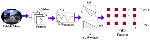
The process of recognizing the vehicle's license plates is initiated with the detection of textural features from the image sequence/video. The proposed BFM using CNL is applied to improve the detection accuracy of the license plate from the frame images. The vehicles are captured and detected through surveillance systems in different instances that rely on better license plate detection accuracy for their textural feature extraction. The license plate detection accuracy is a prominent factor for which the false positive is to be reduced through conventional neural networks. The three main segments such as Preprocessing of the image, number plate detection, and extraction of textural features are performed to achieve maximum accuracy. In Figure 1, the proposed method is illustrated.
The license plate boundary is detected with filtering conditions. The congruent textural features in input frame images are identified and filtered for trained inputs. Based on the image sequence analysis, the similar boundary wavelets detected in the training images help to accurately shape the license plate region from the input images. The conditions of maximum similarity and boundary displacement connectivity are observed from the extracted features and are verified throughout the training process using CNL until reach maximum precision.
Figure 1. Proposed BF Method using CNL
3.1 Preprocessing of the frame images
BFM is the model that makes use of deep learning for textural feature extraction from the input frame images. The video output is analyzed using algorithms/methods for improving the license plate detection precision. CNL is used to train the framing inputs captured from the moving vehicles for accurately identifying vehicle misbehaviors on the roadside. The obtained frame images from moving vehicles using surveillance systems placed in the roadside environment. The textural features are extracted from the frame images for license plate detection and are pursued using deep learning based on the pixel arrangement and intensity in the particular region. Neural learning is used to train the frame input-output for precisely detecting the license plate through correlation from the already trained/identified frame inputs. The process of BFM is pursued to identify, where the congruent textural features are initially identified and filtered. Therefore, the first video output of the license plate $\operatorname{Vid}_o\left(\operatorname{Lics}_{p l t}\right)$ is represented as:
$\operatorname{Vid}_O=\frac{1}{T e} \| \sum_{N=1}^{T e}$ text $_{\text {fex }}\left(\right.$ Lics $\left._{\text {plt }}\right)-F P \|$ (1a)
where,
text $_{\text {fex }}\left(\right.$ Lics $\left._{\text {plt }}\right)=\frac{1}{\sqrt{\pi}} \sum_{N=1}^{T e=0} \frac{\text { Licp }_{\text {boundy }}}{\text { Cong }_{t f}} T e$ (1b)
And,
$F P=\frac{1}{\sqrt{\pi}} \sum_{-\infty}^{\infty} \frac{x_i(T e)+y_i(T e)}{T e}$ (1c)
where, text $_{\text {fex }}\left(\right.$ Lics $\left._{\text {plt }}\right)$ and $F P$ denotes the textural features of the Lics ${ }_{p l t}$ and false positives were identified from the frame images. If $i$ and $L i c p_{\text {boundy }}$ denotes the number of license plate images captured from the current instance and the license plate boundary detected. The textural features are extracted for processing the images based on varying wavelet transform in both x and y coordinates. In this method, the CNL with filtering conditions is used to precisely varying wavelet transform in both x and y coordinates. In this method, the CNL with filtering conditions is used to precisely detect the license plate boundary. If $x$ and $y$ represent the rising and falling edges identified from the frame images at random time intervalsTe. Hence, the images are analyzed for the conditions $x \in[0, \infty]$ and $y \in[-\infty, 0]$ such that the following textural feature extraction equation of the filter is expressed as:
$\begin{aligned} y_N\left[\operatorname{Cong}_{t f}\right]= & 0.5 y_N\left[\operatorname{Cong}_{t f}-1\right] -0.5 y_N\left[\operatorname{Cong}_{t f}-2\right] +x\left[\operatorname{Cong}_{t f}\right]-x\left[\operatorname{Cong}_{t f}-1\right]\end{aligned}$ (2)
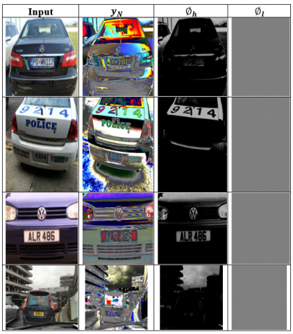
Based on the filtering condition, the initial congruent textural features are filtered and suppressed based on trained frame inputs from the stored dataset. The feature extraction process is illustrated in Figure 2.
Figure 2. Feature extraction process illustration
In the above Figure 2, the frames with $i$ inputs are identified to extract $x$ and $y$ under Licp boundy. Such extractions are validated for each boundary detected in vid $\left(\right.$ Lics $\left._{\text {plt }}\right)$ and text $_{\text {fex }}\left(\right.$ Lics $\left._{\text {plt }}\right)$ are differentiated. The 0.5 -based even distribution for $x$ and $y_N$ are used to detect Licp boundy . Therefore, the normalization process is reliable to improve similarity-based verification. The feature extracted is used to correlate FP across Lics $_{p l t}$ to improve $y_N$. For alltext $t_{\text {fex }}\left(\right.$ Lics $\left._{p l t}\right)+F P$ illustrates a complete sequence of license plate video output analysis for $x$ and $y$ wavelet at different time intervals is expressed as $(N \times T e)$. Here, the variable $N$ indicates the total filtering process of congruent textural features from the instance. Filtering condition is used to reduce the false positives that occur in $\operatorname{Vid}_o\left(\operatorname{Lics}_{p l t}\right)$. False Positives take place in frame inputs due to false boundaries detected at the time of video output analysis in random time intervals. This normalization follows the filtering condition that is described by:
$\left.\begin{array}{rl}\text { Normalization }\left(\text { text }_{\text {fex }}\left(\text { Lics }_{\text {plt }}\right), T e\right)= & \frac{\operatorname{Licp}_{\text {boundy }}(T e)}{\operatorname{Cong}_{\text {tf }}} * \frac{N}{2} S M L_{\text {high }}\left(x_i-y_i\right) \\\text { Normalization }(F P, T e)= & \frac{\text { Te }\left(x_i+y_i\right)}{T e} * \frac{N}{2} S M L_{\text {low }}\left(x_i-y_i\right)\end{array}\right\} $ (3)
where,
$\left.\begin{array}{c}S M L_{\text {high }}=N(T e)\left|\frac{\alpha+\beta}{2}\right| x(T e)_{i-1} \\ \text { and, } \\ S M L_{\text {low }}=N(T e)^{-1}\left|\frac{\alpha+\beta}{2}\right| y(T e)_{i-1}\end{array}\right\}$ (4)
As per the Eqs. (3) and (4), the variables $S M L_{\text {high }}$ and $S M L_{\text {low }}$ represent the high and low similarity based on already trained frame inputs from the dataset. The factor $N(T e)$ and $N(T e)^{-1}$ is the congruent and low textural feature filtering condition based on $S M L_{\text {high }}$ and $S M L_{\text {low }}$ addressed from the inputs. Based on the detection of the license plate boundary (i.e.) $x$ or $y$, the high/low similarity textural features are used to shape the region using the frame inputs. The variables $\alpha$ and $\beta$ represent the training inputs used for the license plate boundary detection. Hence, the normalized wavelet based on $\operatorname{Vid}_o\left(\operatorname{Lics}_{p l t}\right)$ is described as:
$\left.\begin{array}{r}\operatorname{Vid}_o[N(T e)]=\frac{2^{\frac{\alpha+\beta}{2}}[(i \times T e)-N]}{S M L_{\text {high }}-S M L_{\text {low }}} \\ \text { and } \\ \operatorname{Vid}_O[N(T e)]=\frac{2^{\frac{\alpha+\beta}{2}}}{T e}\left[\sum_0^{\infty} \frac{S M L_{\text {high }}[(i \times T e)-N]}{F P}-\sum_{-\infty}^0 \frac{\left.S M L_{\text {low }}[n \times t)-N\right]}{F P}\right]\end{array}\right\}$ (5)
In Eq. (5), the normalized false positive less video output is identified after performing the filtering condition. From this $\operatorname{Vid}_o[N(T e)]$, the two factors namely similarity and boundary displacement are extracted for further analysis. Eqs. (6a) and (6b) used to validate the similarity (Similar(Te)) and boundary displacement $\left(\right.$ Boundry $\left._D(T e)\right)$ in different time interval is as follows:
$\begin{gathered}\operatorname{Similar}(T e)=\frac{1}{2 \pi(N \times T e)}\left|\sum_{N=1}^{\alpha, \beta}\left(x_i-y_i\right) F P^{i-1}\right|, \forall i \in \alpha+\beta\end{gathered}$ (6a)
And,
$\begin{aligned} \operatorname{Boundry}_D(T e)= & -\sum_{i=\emptyset_l}^{\emptyset_h} \operatorname{Similar}(T e) =\log \operatorname{Similar}(T e)_i\end{aligned}$ (6b)
From the above equation, $\emptyset_h$ and $\emptyset_l$ are the high and low similar boundary indices observed from trained frame inputs. The connectivity of maximum $\operatorname{Similar}(T e)$ and Boundry $_D(T e)$ for the $N(T e)$ as in Eq. (6c):
$\operatorname{conect}[N(T e)]=\frac{\text { Boundry }_D(T e)}{\log \left[\frac{\operatorname{Vid}_O\left(\text { Lics }_{\text {plt }}\right)}{\emptyset_h-\emptyset_l}\right]}$ (6c)
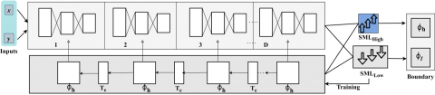
Figure 3. Neural training model for congruency analysis
This connectivity is verified for synchronizing maximum similarity and boundary displacement alone with the different time intervals for precise detection. The classification of maximum and minimum $Similar(T e)$ and $ Boundry_D(T e)$ is performed through the deep learning process. This classification helps to identify the true positives and false positives in both features. In this classification, the textural features are independently analyzed at each level of the neural network followed by classification output. The neural training model is illustrated in Figure 3.
In Figure 3, the neural learning process for $S M L_{\text {High }}$ and $S M L_{\text {Low }}$ are validated across $\emptyset_h$ and $\emptyset_l$ differentiation. This $\emptyset_h$ is equated with $T_e$ to increase the $N\left(T_e\right)$ for $\alpha$ and $\beta$. Here, $\emptyset_h$ with $T_e$ is the $\alpha$ and $\emptyset_h$ with $N\left(T_e\right)^{-1}$ is the $\beta$ under a different $y_N\left[\right.$ cong $\left._{t f}\right]$. The training iterations for congruency are analyzed from the normalized output of $\emptyset_h$ and $\emptyset_l$. If connect $\left[N\left(T_e\right)\right]$ is observed between successive high and low $(x, y)$, the Boundary $D_D$ is detected. This learning does not pursue any conditional validation and thus the $\max D$ is identified from $N\left(T_e\right)$ and $N\left(T_e\right)^{-1}$ variations (Figure 3). The frame inputs and training images are determined as in Eqs. (7a) and (7b) for the conditions of maximum similarity and boundary displacement connectivity.
$\operatorname{CNL}[\operatorname{Similar}(T e, \alpha, \beta)]=-\sum_{i=1}^N T e_i-\sum_{i=1}^{\alpha, \beta} \operatorname{conect}[N(T e)]_i-\sum_{i=1}^N \sum_{j=1}^{\alpha, \beta} T e_i \operatorname{conect}[N(T e)]_i$ (7a)
And,
$\Delta[\operatorname{Similar}(T e, \alpha, \beta)]=\frac{\left(\text { Cong }_{t f}\right)^{-\operatorname{CNL}[\operatorname{Similar(Te)]}}}{\sum_{i=1}^{N \times T e}\left(\text { Cong }_{t f}\right)^{-C N L[\operatorname{Similar}(T e)]_i}}$ (7b)
From the Eqs. (7a) and (7a), CNL[.] indicates the conditional neural learning function for similarity index identification and ∆[.] represents the initial training image at random time intervals. Similarly, the initial training image and already trained frame inputs are comparatively analyzed for final boundary displacement detection $ Boundry_D(T e)$ as:
$\begin{aligned} & C N L\left[\text { Boundry } y_D(T e), \text { Similar }(T e)\right] =\left\{\begin{array}{l}\sum_{i=1}^N T e_i \emptyset_h \frac{1}{S M L_{\text {high }}}, \text { if } \cdot x_i(T e) \in[0, \infty] \\ \sum_{i=1}^N T e_i \emptyset_l \frac{1}{S M L_{l o w}}, \text { if } \cdot y_i(T e) \notin[0, \infty]\end{array}\right.\end{aligned}$ (7c)
And,
$\Delta\left[\text { Boundry }_D(T e), \operatorname{Similar}(T e)\right]=\frac{T P+F P}{F P}$ (7d)
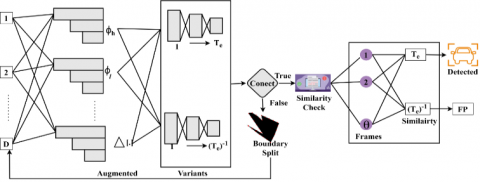
In the above equations, the connectivity of similarity and boundary displacement is verified throughout the process of training until maximum license plate detection precision through deep learning. The maximum precision is achieved using the condition $C N L$ [Boundry ${ }_D(T e)$, Similar $\left.(T e)\right]$ is computed for both $x$ and $y$ coordinates. This computation helps to differentiate the true positive and false positive based on time intervals to achieve the maximum possible detection. Based on the connectivity analysis, conditional neural learning is used for both C N L [.] and $\Delta$ [.] instances. The condition of maximum similarity and boundary displacement connectivity is to reduce condition-failing features. The textural features are extracted from the maximum/minimum similarity and boundary displacement are independently verified for video output analysis. The high/low similarity and boundary displacement connectivity are verified through CNL. The condition-failing features in high and low similarity observed features are administered to prevent false positives and thereby improve true positives. Conditional neural learning ensures filtered textural features between the training inputs for accurate region detection. The filtering is pursued for identifying condition-failing features in frame inputs through deep learning. The aforementioned process is discussed in the following sections. The conditional analysis of the learning process is illustrated in Figure 4.
The conditional validation based on connect $\left[N\left(T_e\right)\right]$ is performed in the above learning process. The $\emptyset_h, \emptyset_l$, and $\Delta$ [.] are the iterated process for $D$ collaboration. The $T_e$ and $\left(T_e\right)^{-1}$ variants are useful in deciding boundary split and similarity checks. In this process, the new boundary split is augmented with new $D$ for $\Delta\left[^{\prime}\right]$ validation. However, the continuous $D$ is yet to be completed from $\theta$ extracts. If $\theta$ satisfies $\left(T_e\right)$ or $\left(T_e\right)^{-1}$ similarity checks, then $D$ is correlated for detecting the boundary of the number plate. The conditional failure requires a boundary similarity check for $\emptyset_h$ or $\emptyset_l$ or both (Figure 4).
Figure 4. Conditional analysis of the learning process
3.2 False positive reduction
The conditional neural learning is defined using two types of segments namely connectivity and no-connectivity between the training images and trained frame inputs. The connectivity is responsible for achieving maximum congruent textural features and boundary displacement whereas in no-connectivity administers low similarity textural features and false positives. The connectivity is performed with $Frame _{\text {in }}=\{1,2, \ldots \theta\}$ set of frame inputs; this frame input is used to extract textural features from all the neural network layers. The Frame $_{\text {in }}$ contains different types of features in different time intervals $T e$. Let $Q$ represent the number of condition-failing features that are present in the frame inputs. Based on the verification, the number of image sequence processing per unit time $P U_{T e}$ such that the license plate detection $(Lics_d)$ is given as:
$\begin{aligned} & Lics_d =\left\{\begin{array}{c} Frame_{\text {in }} \times P U_{T e} \times Te \forall Frame_{\text {in }}:: Te \, and \, Q=0 \\ F P \times \frac{\theta-Q}{Frame_{ in}} \times Te \forall\left(\text { Frame }_{in}, Q\right):: Te \, and \, Q \neq 0\end{array}\right.\end{aligned}$ (8)
Such that,
Frame $_{\text {in }}:: T e=\sum_{i=1}^N P U_{T e}$ (9)
And,
$\left(F r a m e_{i n}, Q\right):: T e=\sum_{i=1}^N P U_{T e}-F P \sum_{i=1}^Q T P$ (10)
where,
$F P=\frac{T P+P U_{T e}}{T P}$ (11)
Based on the above equations, the false positives and condition-failing features from frame inputs in different time intervals. In the above equation, $ Frame_{in}:: T e$ and $(Frame_{in}, Q):: T e$ represents the mapping of the maximum/minimum similarity index addressed from the video processing and false positives in the time interval Te. The license plate detection from the surveillance system is processed based on boundary displacement. In the connectivity observation, the frame input sequence and region are the added-up factors for improving the detection precision using the mapped time interval Te. For training the images, no-connectivity-based detection and filtering are performed. The detection of license plates between $\theta \in$ $Frame_{in}$ and $Q$ is computed through the observation of their connectivity and time metrics. In Eq. (8), the condition $Q>\theta$ produces condition-failing features from the frame inputs. The time metric for filtering the conditionfailing features and the routine connectivity based on $(\theta \times$ $P U_{T e}$ ) are the verifying conditions for detection.
$T e_m=\sum_{i=1}^\theta \frac{Frame_{in}-Q}{F P}$ (12)
And,
$ℸ L i c s_d=\frac{\text { Lics }_d}{(\theta-Q)}\left(\right.$ $Frame_{i n}-F P$ (13)
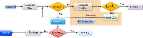
In the above equation, the variable $T e_m$ and $ℸ L i c s_d$ represents the timed connectivity and routine detecting instance. From Eqs. (12) and (13), the precise detection of the license plate is achieved at each instance. This analysis is performed to identify the conditions of $Q \neq 0$ and $Q=0$ in different intervals through recurrent analysis. The false positive reduction process is illustrated in Figure 5.
The FP reduction process is illustrated in the above Figure 5 using $\theta$ as the input. This method first estimates $T_{e_m}$ to verify if it requires $\alpha$ and $\beta$ or both. Depending on the verified condition, if $\tau L i c s_f$ is the required output, and then $\emptyset_h>\emptyset_l$ alone generates precise $D$. This is false positives free requiring an added training. Considering the $\left.\Delta{ }[^{\prime}\right]$ verification, new false positives are presented from causing errors in the further iterations. The case of $Q$ requires new feature verification between different $x$ and $y$ to detect $y_N$. Thus, the different processes of $S M L_{\text {High }}$ and $S M L_{\text {Low }}$ are precise in detecting new $T_{e_m}$ until the FPs are reduced. The recurrent analysis is dependent on filtering sequences from similarity and boundary displacement connectivity verification such that precise detection is achieved using deep learning. If this sequence is observed in any instance, then the license plate detection from $\theta \in Frame_{i n}$ is terminated to reduce no-connectivity observed instances between different frame orientations. The neural learning gives the output of maximum similarity to achieve precise detection to address the false positives. The boundary in the frame inputs is accurately identified and segregated to improve precision. This prevents false positives and condition-failing features by processing frame inputs whereas, the true positive is high.
Figure 5. False positive reduction process
The results and discussion are provided as two sub-sections: experimental and comparative analysis.
4.1 Experimental analysis
Table 1. Boundary displacement outputs
In the experimental analysis, the “Car License Plate Detection” [25] dataset is inherited to validate the proposed method. The dataset provides 433 images with bounded boxes detecting license plates for testing and training. The frames are extracted from PASCAL video format at a rate of 64fps. Each image is annotated with the number of boundaries detected and the actual number. The training iterations pursued is 900 using MATLAB experiment under an epoch of 8/annotation. The optimal image size is 256×256 to 500×300 pixels depending on the resolution and orientation. The experimental results are tabulated for 4 sample inputs in Tables 1 and 2 for different processes undertaken.
Table 2. Boundary detected outputs
4.2 Comparative analysis
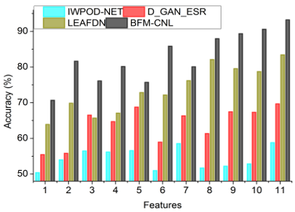
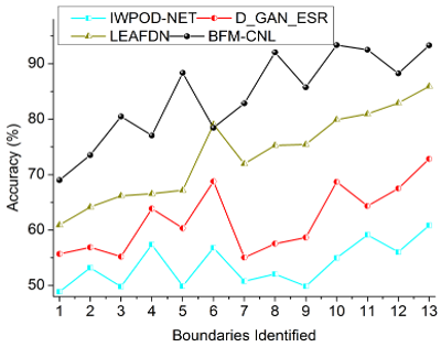
The comparative analysis is performed using accuracy, precision, similarity index, false positives, and analysis time. The highest features extracted are 11 and the boundaries are 13 that are used to estimate the performance variations. The metrics are analyzed comparative with the existing IWPOD-NET [9], D_GAN_ESR [15], and LEAFDN [21] methods.
4.2.1 Accuracy
In this article, the proposed BFM is designed to achieve high license plate detection accuracy based on verifying the connectivity between maximum similarity and boundary displacement from frame inputs and training images represented as in (Refer to Figure 6). The accurate license plate detection with fewer false positives and analysis time is the optimal output here. The congruent textural features are filtered through trained inputs for similarity index identification to reduce analysis time. This proposed method identifies the license plate boundary for filtering conditions using CNL. The license plate is detected from the moving vehicles for authenticating owners based on identifying boundary displacement in each region.
Figure 6. Accuracy
Detecting the pixel arrangement and intensity in a particular region and comparing with trained inputs for similarity analysis. The textural features extracted from the frame images are analyzed in different time intervals to prevent false positives.
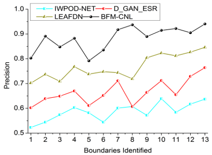
4.2.2 Precision
In this method, textural feature extraction from the video output of the license plate is analyzed to reduce vehicle misdetection (Refer to Figure 7). The high detection precision is achieved through similarity analysis of maximum/minimum similar textural features observed from frames through the proposed method and CNL. The false positives and true positives present in video-based license plate detection are analyzed using the condition $text_{fex}\left(\right.$ $Lics_{plt})+F P$ for minimizing the condition-failing features. In this method, the textural features extraction process initially terminates the displacement-identified frame inputs. The congruent textural features are identified and filtered through CNL to reduce false positives.
This represents maximum similarity and boundary displacement from the raw video frame inputs for accurately detecting license plate region. In this method, the smoothed video-based license plate is generated by identifying the license plate boundary on a gray-scale image sequence to highlight false positives. The acquired information from video-based license plates is analyzed based on extracted textural features through CNL using deep learning resulting in high detection precision with less analysis time. Hence, the condition-succeeding features are recurrently analyzed using filtering conditions to satisfy high precision.
Figure 7. Precision
The similarity and region are verified and compared with already trained frame inputs using CNL for improving accuracy. Hence, high detection accuracy is achieved.
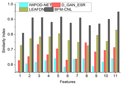
4.2.3 Similarity index
The textural feature obtained from the input video is compared with trained frame images using CNL with less boundary displacement (Refer to Figure 8). The analysis of video outputs is pursued for extracting similar textural features to detect boundaries from the frame images. Hence, the license plate boundary is used to satisfy high accuracy and precision for the detection of license plates using video outputs. In this video-based license plate captured from the moving vehicles is analyzed to identify its boundary and region for which the condition-failing features are reduced. The least possibility of similar boundary indices is detected based on the trained inputs through CNL.
Figure 8. Similarity index
However, the proposed method aided CNL for video output analysis results in high false positives and analysis time. To reduce this complexity use the optimal condition to shape the license plate region. The similarity index identification for region and connectivity output for accurate license plate detection whereas the similarity index detection for false positives is trained to identify boundary. In this method, the CNL is used to improve boundary detection with high similarity indices.
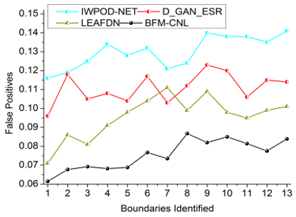
4.2.4 False positives
In this method, the less false positives are achieved by the boundary filtering method and CNL for identifying the region in frame inputs. The textural feature extraction is pursued to merge all the connectivity observed frame inputs for precise detection of a license plate from the original video output. However, the condition-failing features are initially filtered to reduce false positives through CNL. Therefore, additional verification is performed to address false positives in the frame inputs to increase analysis time. The learning process is used to train images for terminating no connectivity between similarity and boundary displacement identified from the original frame image. The least possible false positive is detected to recurrently analyze the video outputs using computer-based algorithms/methods for improving detection precision. The connectivity is verified to accurately identify boundaries through the proposed method. Therefore, similar boundary indices independently identified based on license plate region and connectivity verification which leads to fewer false positives is as illustrated in Figure 9.
Figure 9. False positives
4.2.5 Analysis time
In this method, conditional neural learning is used to identify the condition-failing features from the frame inputs. This is to improve the detection accuracy and precision with BFM as represented in Figure 10. The appropriate connectivity is verified to maintain maximum similarity indices from the training images and is analyzed to achieve fewer false positives and analysis time through the proposed method. In this analysis, the boundary displacement in frame inputs is accurately detected to avoid false positives for preventing complexity. Based on the textural features extracted from video outputs is analyzed using deep learning for achieving high detection precision with less analysis time. The classification of maximum and minimum $Similar(T e)$ and $ Boundry _D(T e)$ is pursued using deep learning to improve accuracy. This classification helps to identify the true positives and false positives between different frame orientations. Thus the proposed method is used to identify such similar boundary indices from frame inputs. Here, the analysis time is less compared to the other factors in this method.
Figure 10. Analysis time
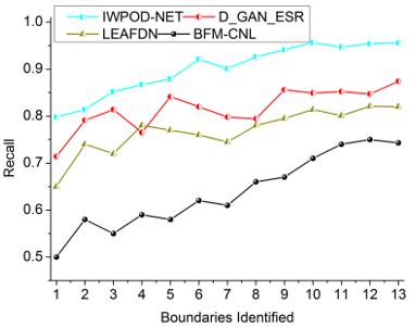
4.2.6 Recall
Figure 11. Recall analysis
The proposed method improves the recall for the varying FPR and boundaries identified. The changes in frame inputs are detected by suppressing the condition-failing features provided the false positives are confined. As the false positives are confined by identifying the displacements using CNL this proposed method is reliable in confining the false positives. Therefore the precision-based training and improvements are validated across multiple boundaries and their corresponding features. This property enhances the recall by reducing the false negatives over true positives. Therefore the different iterations of the CNL training process enhance the recall as presented above (Figure 11).
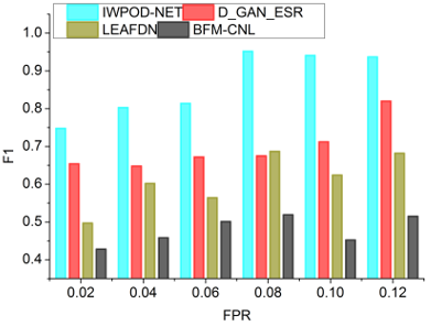
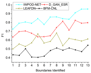
4.2.7 F1-Score
The conditional neural learning process is responsible for improvising the boundary detection of the number plates across various features extracted. Identifying the high and low variations in the features and the false positive rates under multiple boundaries, the proposed method is reliable in improving the F1.
Besides, the similarity measure across different conjugative features improves the true positives. As the precision and recall are improvised by this conditional neural learning, the proposed method is capable of leveraging the F1 score. As the product of precision and recall to the sum of precision and recall is the representation of the F1 score, the proposed method is reliable in achieving the above over different factors. Hence in this case, the proposed method is optimal in improving the F1 for different FPR and boundaries (Figure 12). Table 3 summarize the comparative analysis results.
Figure 12. F1 analysis
Table 3. Comparative analysis results for boundaries identified
|
Metrics |
IWPOD-NET |
D_GAN_ESR |
LEAFDN |
BFM-CNL |
|
Accuracy (%) |
60.57 |
72.83 |
58.93 |
93.318 |
|
Precision |
0.637 |
0.764 |
0.846 |
0.9404 |
|
Similarity Index |
0.667 |
0.742 |
0.846 |
0.9523 |
|
False Positives |
0.141 |
0.114 |
0.101 |
0.0839 |
|
Analysis Time (s) |
0.937 |
0.744 |
0.654 |
0.4851 |
|
Recall |
0.956 |
0.874 |
0.82 |
0.743 |
|
F1 |
0.954 |
0.799 |
0.614 |
0.543 |
Table 4. Individual metric validation for different optimizers
|
Optimizer |
Error |
Accuracy |
Precision |
Recall |
F1 Score |
Execution Time (ms) |
|
ADAM (Benchmark) |
0.11 |
87.6 |
0.90 |
0.85 |
0.87 |
0.248 |
|
CONVBATCH [9] |
0.098 |
87.89 |
0.92 |
0.87 |
0.894 |
0.122 |
|
ADN [15] |
0.078 |
88.47 |
0.95 |
0.88 |
0.941 |
0.139 |
|
AN [21] |
0.045 |
89.54 |
0.94 |
0.92 |
0.925 |
0.208 |
|
NLM |
0.03 |
91.4 |
0.96 |
0.96 |
0.958 |
0.109 |
Table 5. Activation function-based metric validation
|
Activation Function |
Accuracy |
Error |
Precision |
Recall |
F1 Score |
Execution Time (ms) |
|
Tanh |
88.5 |
0.089 |
0.92 |
0.87 |
0.894 |
0.201 |
|
Elu |
87.6 |
0.03 |
0.96 |
0.95 |
0.902 |
0.22 |
|
Softplus |
90.1 |
0.086 |
0.94 |
0.92 |
0.926 |
0.159 |
|
Prelu |
91.4 |
0.11 |
0.92 |
0.956 |
0.959 |
0.187 |
|
Relu |
89.2 |
0.078 |
0.93 |
0.945 |
0.945 |
0.237 |
|
Maxout |
90.1 |
0.069 |
0.94 |
0.939 |
0.956 |
0.231 |
In Table 3 the comparative analysis results for different boundaries identified are presented. The impact of FPR over the boundaries and features is non-congruent in detecting these outputs. Therefore, considering the change between successive features and variations the employed method increases the chances of detection between varying intervals. This result representation also follows the same pattern as the previous method to detect the improvements. The proposed method improves accuracy, precision, and similarity index by 14.6%, 9.57%, and 10.03% respectively. This method reduces false positives and analysis time by 10.43% and 6.28% respectively. Table 4 presents the individual metric validation for different optimizers from the existing to the proposed work.
In Table 4, the different optimizers used in the existing methods are validated for the individual metrics considered. The ADAM optimizer is the benchmark for CONN BATCH [9], adversarial Network (ADN) [15], and the attention network (AN) [21]. Therefore these 4 classifiers are grouped in the above tabulation along the proposed method. In this process the $\Delta$ [similar $\left.\left(T_e, \alpha \beta\right)\right]$ is the verified induced classifier for $\phi_h$ and $\phi_l$ provided $N\left(T_e\right)$ and $N\left(T_e\right)^{-1}$ are high/low or vice versa. Therefore, the classification is influenced by $\alpha$ and $\beta$ under different stages of the number influenced by $\alpha$ and $\beta$ under different stages of the number plate detection process. Followed by the above optimizers, in Table 5, the activation function-based metric validation is presented.
For the different activation functions considered, the discriminative $x$ and $y$ for $\phi_h$ and $\phi_l$ differentiations. In the activation function, $\operatorname{Vid}_o\left[N\left(T_e\right)\right]$ is alone inducted to validate different intervals such that the processes of extraction and detection are robust across $\Delta\left[\right.$ $Boundary_D\left(T_e\right)$, $similar\left.\left(T_e\right)\right]$. Therefore the $\phi_h$ and $\phi_l$ influences each of the classifications highlighted in the detection process. This further impacts the execution based on different $\phi_h$ and $\phi_l$ entries increasing the accuracy factor. Table 6 analyzes the error, validation, and evaluation of the different activation functions for different learning rates.
Table 6. Error, validation, and evaluation of different activation functions under learning rates
|
Activation Function |
Learning Rate |
Error |
Validation |
Evaluation |
|
Tanh |
0.2 |
0.11 |
0.59 |
0.741 |
|
0.4 |
0.101 |
0.62 |
0.784 |
|
|
0.6 |
0.098 |
0.68 |
0.841 |
|
|
0.4 |
0.095 |
0.74 |
0.854 |
|
|
1 |
0.09 |
0.81 |
0.874 |
|
|
Elu |
0.2 |
0.108 |
0.79 |
0.891 |
|
0.4 |
0.105 |
0.81 |
0.921 |
|
|
0.6 |
0.098 |
0.85 |
0.947 |
|
|
0.4 |
0.095 |
0.87 |
0.963 |
|
|
1 |
0.093 |
0.90 |
0.974 |
|
|
Softplus |
0.2 |
0.098 |
0.85 |
0.654 |
|
0.4 |
0.096 |
0.87 |
0.714 |
|
|
0.6 |
0.0958 |
0.885 |
0.789 |
|
|
0.4 |
0.0927 |
0.897 |
0.801 |
|
|
1 |
0.0901 |
0.901 |
0.821 |
|
|
Prelu |
0.2 |
0.121 |
0.4 |
0.698 |
|
0.4 |
0.12 |
0.45 |
0.745 |
|
|
0.6 |
0.118 |
0.487 |
0.854 |
|
|
0.4 |
0.105 |
0.496 |
0.874 |
|
|
1 |
0.098 |
0.524 |
0.965 |
|
|
Relu |
0.2 |
0.124 |
0.621 |
0.987 |
|
0.4 |
0.121 |
0.635 |
0.925 |
|
|
0.6 |
0.105 |
0.741 |
0.954 |
|
|
0.4 |
0.095 |
0.782 |
0.974 |
|
|
1 |
0.092 |
0.814 |
0.987 |
|
|
Maxout |
0.2 |
0.13 |
0.748 |
0.897 |
|
0.4 |
0.128 |
0.847 |
0.921 |
|
|
0.6 |
0.125 |
0.868 |
0.965 |
|
|
0.4 |
0.104 |
0.891 |
0.984 |
|
|
1 |
0.097 |
0.897 |
0.989 |
Table 7. Overall and average accuracy analysis of different activation functions
|
Activation Function |
Parameter |
Accuracy |
|
Tanh |
OA |
0.915 |
|
AA |
0.885 |
|
|
Elu |
OA |
0.924 |
|
AA |
0.876 |
|
|
Softplus |
OA |
0.934 |
|
AA |
0.901 |
|
|
Prelu |
OA |
0.928 |
|
AA |
0.914 |
|
|
Relu |
OA |
0.951 |
|
AA |
0.892 |
|
|
Maxout |
OA |
0.938 |
|
AA |
0.901 |
In Table 6, a detailed analysis of the activation functions under different learning rates is presented. The error validation and evaluation for different activation functions and learning rate is optimized using identifiable $\phi_h$ and $\phi_l$. The $\alpha$ and $\beta$ are the learning rate-improving factors based on FP occurrences. Hence in such cases, the evaluation is instigated by normalization $\left(F P, T_e\right)$ until the error is reduced. The loss impacts the validation using $\alpha$ or $\beta$ whereas both metrics are considered for evaluation through $N\left(T_e\right)$ and $N\left(T_e\right)^{-1}$. Each activation function utilizes this output to improvise the metrics under different rates. The overall and average accuracy of different activation functions are analyzed in Table 7.
In Table 7, the OA and AA analysis for different functions is presented. Each function is unique in selecting $\phi_h$ and $\phi_l$ with and without normalization. The number of execution steps is validated across different $S M L_{\text {high }}$ and $S M L_{\text {low }}$ for $\operatorname{conect}\left[N\left(T_e\right)\right]$. This is the key factor for detecting maximum/minimum classification features for $\alpha$ and $\beta$ inputs stabilizing OA. The AA is the mean of different OA under varying learning rates and $\left(\phi_h+\phi_l\right)$ variations.
To improve the detection accuracy of vehicle license plates, this article proposed and briefed the boundary filtering method using conditional neural learning. This method first extracts the textural features to identify the congruent features based on similarity. The similarity index-based validations are performed to differentiate high and low feasible feature detection between the edges of the input image. The conditional neural learning filters the high similarity features to improve the training and detection precision. In this conditional assessment, the texture congruency is verified using similarity and displacement factors. These factors are augmented to add up the boundary feature continuity that improves the detection accuracy. As the feature augmentation based on similarity index is pursued the highest precision in detecting the boundary is achieved. From the comparative analysis, the proposed method improves accuracy, precision, and similarity index by 11.3%, 10.23%, and 11.06% respectively for the highest feature. The advantage of boundary feature continuity turns out to be less feasible for color variant features. This requires an equalization process before its edge detection process; this constructive feature is planned to be incorporated in the future with dynamic concerns.
[1] Ahn, H., Cho, H.J. (2023). Research of automatic recognition of car license plates based on deep learning for convergence traffic control system. Personal and Ubiquitous Computing, 27(3): 1139-1148. https://doi.org/10.1007/s00779-020-01514-z
[2] Pattanaik, A., Balabantaray, R.C. (2023). Enhancement of license plate recognition performance using Xception with Mish activation function. Multimedia Tools and Applications, 82(11): 16793-16815. https://doi.org/10.1007/s11042-022-13922-9
[3] Yu, H., Wang, X., Shao, Y., Qin, F., Chen, B., Gong, S. (2022). Research on license plate location and recognition in complex environment. Journal of Real-Time Image Processing, 19(4): 823-837. https://doi.org/10.1007/s11554-022-01225-z
[4] Huang, Q., Cai, Z., Lan, T. (2021). A single neural network for mixed style license plate detection and recognition. IEEE Access, 9: 21777-21785. https://doi.org/10.1109/ACCESS.2021.3055243
[5] Shashirangana, J., Padmasiri, H., Meedeniya, D., Perera, C. (2020). Automated license plate recognition: A survey on methods and techniques. IEEE Access, 9: 11203-11225. https://doi.org/10.1109/ACCESS.2020.3047929
[6] Shahidi Zandi, M., Rajabi, R. (2022). Deep learning based framework for Iranian license plate detection and recognition. Multimedia Tools and Applications, 81(11): 15841-15858. https://doi.org/10.1007/s11042-022-12023-x
[7] Muhammad, J., Altun, H. (2023). Guiding genetic search algorithm with ANN based fitness function: A case study using structured HOG descriptors for license plate detection. Multimedia Tools and Applications, 82(12): 17979-17997. https://doi.org/10.1007/s11042-022-14195-y
[8] Zhang, C., Wang, Q., Li, X. (2021). V-LPDR: Towards a unified framework for license plate detection, tracking, and recognition in real-world traffic videos. Neurocomputing, 449: 189-206. https://doi.org/10.1016/j.neucom.2021.03.103
[9] Silva, S.M., Jung, C.R. (2021). A flexible approach for automatic license plate recognition in unconstrained scenarios. IEEE Transactions on Intelligent Transportation Systems, 23(6): 5693-5703. https://doi.org/10.1109/TITS.2021.3055946
[10] Pan, X., Li, S., Li, R., Sun, N. (2022). A hybrid deep learning algorithm for the license plate detection and recognition in vehicle-to-vehicle communications. IEEE Transactions on Intelligent Transportation Systems, 23(12): 23447-23458. https://doi.org/10.1109/TITS.2022.3213018
[11] Jia, W., Xie, M. (2023). An efficient license plate detection approach with deep convolutional neural networks in unconstrained scenarios. IEEE Access. https://doi.org/10.1109/ACCESS.2023.3301122
[12] Shi, H., Zhao, D. (2023). License plate recognition system based on improved YOLOv5 and GRU. IEEE Access, 11: 10429-10439. https://doi.org/10.1109/ACCESS.2023.3240439
[13] Pan, S., Chen, S.B., Luo, B. (2023). A super-resolution-based license plate recognition method for remote surveillance. Journal of Visual Communication and Image Representation, 94: 103844. https://doi.org/10.1016/j.jvcir.2023.103844
[14] Zhang, S., Lu, X., Lu, Z. (2023). Improved CNN-based CatBoost model for license plate remote sensing image classification. Signal Processing, 213: 109196. https://doi.org/10.1016/j.sigpro.2023.109196
[15] Hamdi, A., Chan, Y.K., Koo, V.C. (2021). A new image enhancement and super resolution technique for license plate recognition. Heliyon, 7(11).
[16] Cao, Y. (2024). Investigation of a convolutional neural network-based approach for license plate detection. Journal of Optics, 53(1): 697-703. https://doi.org/10.1007/s12596-023-01243-5
[17] Gautam, A., Rana, D., Aggarwal, S., Bhosle, S., Sharma, H. (2023). Deep learning approach to automatically recognise license number plates. Multimedia Tools and Applications, 82(20): 31487-31504. https://doi.org/10.1007/s11042-023-15020-w
[18] Pham, T.A. (2023). Effective deep neural networks for license plate detection and recognition. The Visual Computer, 39(3): 927-941. https://doi.org/10.1007/s00371-021-02375-0
[19] Qin, S., Liu, S. (2022). Towards end-to-end car license plate location and recognition in unconstrained scenarios. Neural Computing and Applications, 34(24): 21551-21566. https://doi.org/10.1007/s00521-021-06147-8
[20] Wang, Q., Lu, X., Zhang, C., Yuan, Y., Li, X. (2022). LSV-LP: Large-scale video-based license plate detection and recognition. IEEE Transactions on Pattern Analysis and Machine Intelligence, 45(1): 752-767. https://doi.org/10.1109/TPAMI.2022.3153691
[21] Seo, T.M., Kang, D.J. (2022). A robust layout-independent license plate detection and recognition model based on attention method. IEEE Access, 10: 57427-57436. https://doi.org/10.1109/ACCESS.2022.3178192
[22] Saitov, I., Filchenkov, A. (2023). CIS multilingual license plate detection and recognition based on convolutional and transformer neural networks. Procedia Computer Science, 229: 149-157. https://doi.org/10.1016/j.procs.2023.12.016
[23] Shafi, I., Hussain, I., Ahmad, J., Kim, P.W., Choi, G.S., Ashraf, I., Din, S. (2022). License plate identification and recognition in a non-standard environment using neural pattern matching. Complex & Intelligent Systems, 8(5): 3627-3639. https://doi.org/10.1007/s40747-021-00419-5
[24] Maltsev, A., Lebedev, R., Khanzhina, N. (2021). On realistic generation of new format license plate on vehicle images. Procedia Computer Science, 193: 190-199. https://doi.org/10.1016/j.procs.2021.10.019
[25] Andrew Mvd. Car Plate Detection Dataset. https://www.kaggle.com/datasets/andrewmvd/car-plate-detection, accessed on Feb. 27, 2024.