Ying Chen![]()
© 2024 The author. This article is published by IIETA and is licensed under the CC BY 4.0 license (http://creativecommons.org/licenses/by/4.0/).
OPEN ACCESS
In the modern logistics industry, the rapid growth of e-commerce has made real-time load monitoring of delivery vehicles a critical factor in ensuring transportation efficiency and safety. However, traditional load monitoring methods are often hindered by delayed data acquisition and insufficient accuracy, making them inadequate for the high demands of efficient and precise logistics operations. Recently, with advancements in deep learning-based image analysis, image-based load monitoring methods have gained attention. However, existing studies face challenges in robustness and real-time performance, particularly in dynamic and complex environments. To address these issues, this paper proposes a real-time load monitoring method for logistics delivery vehicles based on deep learning techniques, focusing on three core technologies: subpixel edge detection in 2D images, interpolation between consecutive image frames, and real-time load volume calculation. This research aims to enhance the accuracy and real-time capabilities of load monitoring, thereby advancing the intelligent development of the logistics industry.
logistics delivery vehicles, real-time load monitoring, deep learning, subpixel edge detection, interpolation, load volume calculation
In the modern logistics industry, load monitoring of delivery vehicles is a crucial aspect of ensuring transportation efficiency and safety [1-3]. With the rapid development of e-commerce, the demand for logistics delivery has significantly increased, making the real-time monitoring of vehicle loads in complex and variable environments an urgent issue to be addressed [4-6]. Traditional load monitoring methods largely rely on vehicle-installed sensors or manual records. However, these methods suffer from issues such as delayed data acquisition and significant errors, making them inadequate for the demands of efficient and precise logistics operations [7, 8]. With the rapid development of deep learning and computer vision technologies, utilizing image analysis methods for real-time load monitoring of logistics delivery vehicles has become a forward-looking solution.
The significance of this research lies in exploring and developing a real-time load monitoring method based on image deep learning technology. By processing and analyzing images of logistics delivery vehicles, this method can accurately identify and calculate the current load condition of the vehicle [9-11]. This approach not only improves the accuracy of load monitoring but also greatly reduces manual involvement, thereby enhancing the level of intelligence across the entire logistics delivery chain [12, 13]. Moreover, by monitoring vehicle loads in real time, it is possible to effectively prevent issues such as overloading and load imbalance, thereby improving safety during the transportation process and reducing transportation risks.
Although some studies have attempted to apply image processing technology to the load monitoring of logistics vehicles, most of these methods still exhibit many shortcomings in practical applications [14-18]. For example, existing methods often lack sufficient robustness when processing images in dynamic and complex environments, making them susceptible to external factors such as lighting and occlusion, which can result in inaccurate monitoring results. Furthermore, the real-time performance of image processing still needs improvement, as it currently fails to meet the high-efficiency requirements of logistics delivery processes [19-21]. Therefore, it is particularly necessary to study more accurate image analysis technologies with real-time processing capabilities to address these deficiencies.
The main content of this research includes three parts. First, for real-time load monitoring of logistics delivery vehicles, a two-dimensional image subpixel edge detection method is proposed to improve the accuracy of load identification. Second, a fitting interpolation technique between consecutive image frames is studied to enhance the continuity and consistency of image data. Finally, through the analysis and processing of image data, a real-time load volume calculation method based on images is proposed. This research not only fills the gap in existing technologies but also provides new technical pathways and theoretical support for the intelligent development of the logistics industry in the future.
In real-time load monitoring of logistics delivery vehicles, accurately obtaining load information is a key aspect of achieving precise monitoring and intelligent management. The subpixel edge detection technology in 2D images plays a crucial role in this process. Due to the typically complex shape and distribution of vehicle loads, traditional image processing methods struggle to accurately locate the edges of objects at the pixel level, thereby affecting the accuracy of load calculations. Through subpixel edge detection technology, it is possible to enhance the precision of load measurement and reduce errors caused by edge blurring or misjudgment. This is particularly important in dynamic and complex logistics delivery environments, where accurate edge detection helps to address challenges such as lighting variations and occlusions.
The spline fitting interpolation problem for edge points in 2D images in real-time load monitoring of logistics delivery vehicles involves generating continuous and smooth edge curves from the results of edge detection. Specifically, due to the potential discontinuities or noise interference in the actual edge points obtained from images, directly using these points for load calculations can result in insufficient accuracy. Therefore, spline fitting interpolation technology is introduced to generate smooth curves between these discrete edge points, making the edge information more complete and accurate. The core of this problem lies in selecting the appropriate spline function and performing effective interpolation, ensuring the continuity and smoothness of the edge curve in the dynamic and complex logistics environment, thereby providing reliable foundational data for subsequent load calculations. Specifically, given the function d(a) with function values b0,b1,...,bv at v + m nodes a0,a1,...,av, the task is to find a cubic spline function t(a) that satisfies:
$t\left(a_k\right)=b_k, u=0,1, \cdots, v$ (1)
In the spline fitting interpolation problem for edge points in 2D images in real-time load monitoring of logistics delivery vehicles, the choice of boundary conditions directly affects the smoothness and accuracy of the edge curve. Considering the specific requirements of this study, the following boundary conditions are adopted:
(1) Fixed boundary conditions: At the two boundary nodes of the image, the first derivative of the edge curve is set to a fixed value, i.e., t′(a0) = l0 and t′(av) = lv. This condition is suitable for scenarios in logistics vehicle load monitoring images where the direction and trend of the edge points are clearly defined. By specifying fixed derivative values, the slope of the edge curve at the boundary is ensured to be consistent with the actual physical characteristics, thereby accurately reflecting the edge changes of the vehicle load.
(2) Second boundary conditions: This boundary condition sets the second derivative at the boundary nodes to a fixed value, i.e., t′′(a0) = l0 and t′′(av) = lv. Particularly, when l0 and lv are zero, it is referred to as the natural boundary condition. This condition is particularly common in logistics delivery vehicle load monitoring, as in practical applications, the edge curve at the boundary usually tends to flatten, with the second derivative being zero. This natural boundary condition helps to generate a smooth edge curve, avoiding unnatural bends at the boundary, thereby improving the accuracy of load monitoring.
(3) Periodic boundary conditions: This condition requires that the values of the first and second derivatives at the starting and ending boundaries of the image are equal, i.e., t′(a0) = t′(av) and t′′(a0) = t′′(av). For logistics delivery vehicle load monitoring images, this condition can be applied to scenarios where the load distribution is periodic or symmetric, ensuring consistency of the edge curve at the starting and ending points of the image, thereby reducing calculation errors and discontinuities.
The process of determining the cubic spline function expression mainly includes the following key steps:
The extraction of edge points is fundamental. Through subpixel edge detection technology, the coordinates of the edge points in the load images of logistics delivery vehicles are accurately obtained. These edge points are usually discrete and may contain some noise, requiring smoothing in subsequent processing. Specifically, in the given interval [a, b], there are:
$x_0=a_0<a_1<\cdots<a_V=y$ (2)
Given constants b0,b1,...,bV, assuming the cubic spline function is represented by T3, a function can be constructed to satisfy:
$T(a) \in T_3\left(a_1, a_2, \cdots, a_V\right)$ (3)
The constructed function satisfies the following interpolation conditions:
$T\left(a_k\right)=b_k, k=0,1, \ldots, V$ (4)
For each pair of adjacent edge points, a cubic polynomial needs to be constructed. This polynomial is spliced at all edge points to generate a continuous and smooth curve. Specifically, let Lk represent T″(ak)(k =0,1,...,V). Since T(a) is a piecewise cubic polynomial in the interval nodes, T″(a) changes linearly within the segment interval [ak-1, ak]. Let gk = ak-ak-1, and the linear interpolation function can be obtained from the two points (ak-1, Lk-1) and (ak-1, Lk):
$T^{\prime \prime}(a)=L_{k-1} \frac{a_k-a}{g_k}+L_k \frac{a-a_{k-1}}{g_k}\left(a_{k-1} \leq a \leq a_k\right)$ (5)
Integrating the above equation twice yields the expression for T(a) within the segment interval [ak-1, ak] and the integral constant. When a ∈ [ak-1, ak], we have:
$\begin{aligned} T(a)= & L_{k-1} \frac{\left(a_k-a\right)^3}{6 g_k}+M_j \frac{\left(a-a_{k-1}\right)^3}{6 g_k} \\ & +\left(b_{k-1}-\frac{L_{k-1} g_k^2}{6}\right) \frac{a_k-a}{g_k}+\left(b_k-\frac{L_k g_k^2}{6}\right) \frac{a-a_{k-1}}{g_k} \\ T^{\prime}(a) & =-L_{k-1} \frac{\left(a_k-a\right)^2}{2 g_k}+L_k \frac{\left(a-a_{k-1}\right)^2}{2 g_k} \\ & +\frac{b_k-b_{k-1}}{g_k}-\frac{L_k-L_{k-1}}{6} g_k\end{aligned}$ (6)
Based on the above equation, to obtain T(a), it is necessary to determine each Lk(k=0,1,...,V) according to the continuity and smoothness conditions at the spline nodes, namely:
$T^{\prime}\left(a_k-0\right)=T^{\prime}\left(a_k+0\right)$ (7)
According to the above equation, we have:
$\begin{aligned} & T^{\prime}\left(a_k-0\right)=\frac{g_k}{6} L_{k-1}+\frac{h_j}{3} M_j+\frac{y_j-y_{j-1}}{h_j} \\ & T^{\prime \prime}\left(a_k+0\right)=-\frac{g_{k+1}}{3} L_k+\frac{g_{k+1}}{6} L_{k+1}+\frac{b_k-b_{k-1}}{g_k}\end{aligned}$ (8)
Further, the following equation can be derived:
$\begin{aligned} & \frac{g_k}{6} L_{k-1}+\frac{g_k+g_{k+1}}{3} L_k+\frac{g_{k+1}}{6} L_{k+1} \\ & =\frac{b_{k+1}-b_k}{g_{k+1}}-\frac{b_k-b_{k-1}}{g_k}(k=1, \cdots, V-1)\end{aligned}$ (9)
The above equation provides V-1 equations containing V + m unknowns Lk(k=0,1,...,V). However, to uniquely determine each Lk(k=0,1,...,V), it is necessary to supplement the conditions of the natural spline function. First, the value of the spline function at each edge point should be consistent with the original data points. Second, ensure that the first and second derivatives of each polynomial are continuous at the boundary points. Third, set the values of the first or second derivatives at the first and last nodes according to the chosen boundary conditions. By these conditions, a set of linear equations is established as follows:
$\left\{\begin{array}{l}2 L_0+\eta_0 L_1=f_0 \\ \omega_V L_{V-1}+2 L_V=f_V\end{array}\right.$ (10)
The linear equation system determined based on the above equation is:
$\left[\begin{array}{ccccccccc}2 & \eta_0 & & & & & & & \\ \omega_1 & 2 & \eta_1 & & & & & P & \\ & \omega_2 & 2 & \eta_2 & & & & & \\ & & \bullet & \bullet & \bullet & & & & \\ & & & \bullet & \bullet & \bullet & & & \\ & & & & \bullet & \bullet & \bullet & & \\ & P & & & & \omega_{V-2} & 2 & \eta_{V-2} & \\ & & & & & & \omega_{V-1} & 2 & \eta_{V-1} \\ & & & & & & & \omega_V & 2\end{array}\right]\left[\begin{array}{c}L_0 \\ L_1 \\ L_2 \\ \bullet \\ \bullet \\ \bullet \\ L_{V-2} \\ L_{V-1} \\ L_V\end{array}\right]=\left[\begin{array}{c}f_0 \\ f_1 \\ f_2 \\ \bullet \\ \bullet \\ \bullet \\ f_{V-2} \\ f_{V-1} \\ f_V\end{array}\right]$ (11)
Solving the above equation yields the expression for the cubic spline interpolation function.
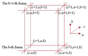
In real-time load monitoring of logistics delivery vehicles, sub-pixel edge localization of two-dimensional images provides precise edge point information. However, in practical applications, load monitoring often requires processing image data of consecutive frames to ensure accurate monitoring of dynamically changing loads. Due to the limited time interval between consecutive frames, especially in high-speed shooting or fast-moving load scenarios, there may be significant displacement or change between frames. This results in a mismatch between the spatial resolution of consecutive frames and the image resolution within a single frame. Similar to the problem of axial spacing in three-dimensional scanning tomography data being much greater than the horizontal distance between pixels, this mismatch affects the accuracy and continuity of load monitoring. Figure 1 shows the schematic diagram of consecutive frame matching in real-time load monitoring of logistics delivery vehicles.
Figure 1. Schematic diagram of consecutive frame matching in real-time load monitoring of logistics delivery vehicles
Therefore, after completing sub-pixel edge localization of two-dimensional images, it is necessary to perform interpolation between consecutive frames of images. This process generates interpolated frames between adjacent frames, making the spatial resolution of consecutive frames more consistent, thus compensating for the missing information between frames. Through interpolation, the dynamic changes in vehicle loads can be better captured, avoiding monitoring errors caused by frame jumps or displacements, and ensuring the continuity and smoothness of load calculation. Especially in complex logistics environments, where the distribution and shape of the load may change rapidly, interpolation between consecutive frames can provide more accurate load information, enhancing the reliability of real-time monitoring. Figure 2 shows the schematic diagram of consecutive frame monitoring.
Figure 2. Schematic diagram of consecutive frame monitoring
During actual monitoring, the shape and distribution of the load may change significantly between consecutive frames, especially in scenarios where the vehicle load undergoes substantial dynamic changes. Although traditional linear interpolation methods can fill in the information gaps between consecutive frames, they cannot effectively capture and interpolate the complex contour shapes of inter-layer images, leading to discontinuities or blurring in the contour edges of the interpolated images, thereby affecting the accuracy of load monitoring. To solve this problem, this paper introduces a shape-based interpolation algorithm. The core idea of this algorithm is to construct a distance function that converts the pixel gray values in a binary image into the shortest distance values from the pixel to the edge point. This distance function is used as the interpolation criterion to generate inter-layer interpolated images. Compared to linear interpolation, this method focuses more on the continuity and shape preservation of contour edges, generating more accurate and continuous inter-layer images, ensuring precise positioning and transition of load edges, thereby enhancing the overall monitoring effect of vehicle loads.
One of the key steps in the shape-based interpolation method is to construct a distance function suitable for this scenario to ensure smooth transitions of contour edges between consecutive frames. The distance function measures the shortest distance between each pixel and the edge point to generate interpolated images. In the image processing of logistics delivery vehicle load monitoring, this distance function can be defined as Euclidean distance, city block distance, or chessboard distance, each of which is suitable for different image characteristics. By calculating the shortest distance from the pixel position of each foreground point to the background point, i.e., the shortest distance from the load edge point to the area outside the load, and storing these distances, the original binary edge image can be converted into a grayscale image. These grayscale values represent the shortest distance between each pixel and the nearest background pixel. These distance values are then used as the interpolation criterion to generate interpolated images between consecutive frames. Specifically, the distance function characterizes the relationship between all points O, P, and E:
The specific interpolation steps are as follows:
(1) Segment the load monitoring image of each frame. This paper adopts a thresholding method to quickly separate the load area from the background according to the characteristics of the logistics load. Through thresholding segmentation, a clear binary image can be obtained, clearly identifying the contour edges of the load.
(2) Perform distance transformation on the segmented binary image, i.e., calculate the shortest distance from each foreground pixel to the nearest background pixel, and generate a distance matrix F(a,b,c). This matrix records the distance information of each pixel to the edge, laying the foundation for subsequent shape interpolation.
(3) After obtaining the distance matrix F(a,b,c), perform interpolation calculations. This process can be achieved through erosion and dilation operations in mathematical morphology. Specifically, by performing erosion and dilation on the target template, it is deformed to gradually generate contour point information of the intermediate frame's tomographic image. After each iteration, a new distance mapping image of the interpolated layer can be obtained, gradually achieving the transition of contours between frames.
Assuming that the composite operation of dilation and iteration is represented by F|γ, the result of the v-th iteration is:
$F_2^{(v)}(a, b, c)=(F \mid \gamma)\left[F_2^{(v)}(a, b, c)\right]$ (12)
(4) Since the distance mapping image contains the fusion information of contour shapes between the two original frames, the interpolated image between them can be generated through this mapping image. This step ensures a natural transition from the target shape of one frame to the target shape of the next frame, thereby achieving high-precision continuous image processing in the monitoring of logistics delivery vehicle loads, ensuring accurate monitoring of load changes.
In the real-time load monitoring of logistics delivery vehicles, the aforementioned sub-pixel edge detection of two-dimensional images and fitting interpolation between consecutive frames can accurately capture and generate edge contour information of the load. However, to further achieve the calculation of the actual area and volume of the load, it is necessary to convert these processed image data into actual physical dimensions, thereby quantitatively evaluating the vehicle load.
After image processing is completed, the resulting load contours are usually represented in pixel units. To convert these pixel areas into actual physical areas, a scale factor is introduced, which is derived from the camera's calibration results. Specifically, by using a reference object or calibration board with known dimensions within the camera's shooting range, the actual physical length corresponding to each pixel is determined, thereby calculating the proportional relationship between the pixel area and the actual area. Using this scale factor, the load pixel area calculated from the image is converted into the actual physical area. Next, the load volume is calculated. In a two-dimensional image, calculating the load volume requires combining depth or height information from multiple frames. For real-time load monitoring, depth information for the load at different positions can be obtained through the interpolation results between consecutive frames. These areas are then multiplied by their corresponding height or depth values, and the products are integrated or summed to calculate the total load volume.
First, by analyzing the captured images, the number of pixels along the load's edge in the image is determined, such as the load's width pixel count SL. Next, this pixel count is divided by the entire image's resolution FBL, namely the total pixel count corresponding to the image width, to calculate a scale factor RA.
$R A=\frac{S L}{F B L}$ (13)
This scale factor represents the relationship between the load width in the image and the entire frame width. Then, using the known actual frame width sQ, the actual load width can be calculated using the following formula:
$Q=\frac{S L}{F B L} \cdot S I N\left(\frac{2}{D P N}\right) \cdot D E \cdot 2$ (14)
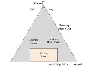
Figure 3 gives a schematic diagram showing the relationship between the camera and the vehicle load. The calculation of the load height depends on the camera's field of view and the distance between the camera and the load. Specifically, the load height can be obtained by multiplying the cosine value of half the DPN by the depth value from the camera to the image boundary and then subtracting the depth value YDE of the load. This process considers changes in the camera's viewing angle and the load's position in the image, thereby accurately calculating the load height G. The formula can be expressed as:
$G=\operatorname{COS}\left(\frac{2}{D P N}\right) \cdot D E-Y D E$ (15)
Figure 3. Relationship between the camera and the vehicle load
After obtaining the actual load width Q and height G, the next step is to calculate its volume. Typically, the load volume can be calculated using the following formula: V = Q × M × G, where M represents the load length. The calculation method for length M is similar to that of width Q, which is also calculated based on the ratio of pixel count to image resolution and then combined with actual measurement data. By multiplying the load's width, length, and height, the total load volume can be obtained.
As the vehicle moves during transportation, the load's shape and position may change, necessitating real-time updates to the load's area and volume calculations. Using image deep learning technology, the load contour changes can be automatically recognized and tracked, and the calculation results can be quickly updated. This process can provide real-time load information to assist the logistics management system in making dynamic adjustments, such as optimizing loading schemes, predicting the stability of cargo placement, or assessing the uniformity of vehicle load distribution.
Based on the experimental results from Table 1 and Table 2, it can be observed that the method after sub-pixel edge detection of two-dimensional images significantly reduces the average error and error range across all load volume ranges. In the 100~150 cm load volume range, the average error after detection decreases from 0.32 to 0.09, and the error range drops from 3.89 to 1.22. Additionally, the calculation time slightly increases after sub-pixel edge detection but remains within a range of 10.4 to 13.5 seconds, slightly higher than the 4.2 to 5.2 seconds before detection. The experimental results indicate that the proposed two-dimensional image sub-pixel edge detection method significantly improves the accuracy of load recognition, particularly in smaller load volume ranges. This improvement is primarily reflected in the lower average error and error range, demonstrating the method's effectiveness in practical applications. However, due to the increased calculation time, while this method is more suitable for scenarios requiring high precision, it may necessitate a trade-off between accuracy and efficiency in time-sensitive applications.
Based on the experimental results from Table 3, different load distances and minimum voxel settings have a significant impact on the calculation time and error range of the proposed method. Within the same load volume range of 350~500 cm, as the load distance increases, the calculation time gradually increases. For example, when the load distance is 100, the calculation time ranges from 15.2 seconds to 19.1 seconds; however, when the load distance increases to 300, the calculation time rises to 18.8 seconds to 22.5 seconds. At the same time, the error range also varies under different conditions, generally increasing with the increase of the minimum voxel. However, when the load distance is 300 and the minimum voxel is 8, the error range actually decreases, differing from the cases where the minimum voxel is 2 and 4. The experimental results show that the choice of load distance and minimum voxel directly affects the performance of the load volume calculation method. Shorter load distances and smaller minimum voxels can significantly reduce calculation time but may lead to an increase in the error range. On the contrary, larger load distances increase calculation time, and in some cases, the error range decreases. This indicates that in practical applications, it is necessary to comprehensively consider the configuration of load distance and minimum voxel to find the optimal balance between calculation efficiency and error range. Particularly when the load distance is large, reasonably adjusting the minimum voxel can optimize the error performance while maintaining relatively short calculation times.
Table 4 shows the comparison of the average error range of the proposed method, Random Forest, and LMedS methods under different combinations of load volume and load distance. Overall, the average error range of the proposed method is slightly higher than that of the Random Forest method in each combination of load volume and load distance but lower than that of the LMedS method. For example, in the 100~150 cm load volume range and 100 load distance, the error range of the proposed method is 1.02, while Random Forest and LMedS are 0.73 and 0.78, respectively. As the load distance increases, the error range of the proposed method also increases. Particularly when the load volume is greater than 500 cm and the load distance is 300, the error range reaches 1.42, the same as Random Forest, but still better than LMedS’s 1.67. The experimental results indicate that although the proposed two-dimensional image sub-pixel edge detection method is slightly inferior to Random Forest in terms of error range, its error range remains relatively stable and is superior to the LMedS method. This means that the proposed method can provide more consistent performance in complex scenarios while maintaining high accuracy, particularly excelling in large load volumes and long load distances.
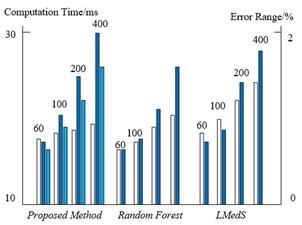
This paper compares the performance of the proposed method, Random Forest, and LMedS algorithms under different load volumes through Figure 4. The dark blue bars represent the error magnitude, the light blue bars represent the error magnitude after adjusting the voxel size, and the white hollow bars represent the changes in computation time. It can be observed that the computation time for the Random Forest and LMedS algorithms significantly increases as the load volume increases, especially for the LMedS algorithm under large volume loads, whereas the proposed method shows relatively stable computation time that does not significantly increase with load volume. Additionally, under small load volumes, the computation speed differences among the three algorithms are not significant, but as the load volume increases, the proposed method demonstrates up to a 15% advantage in computation efficiency. In terms of error, the error magnitude of the proposed method before adjusting the voxel size is slightly higher than the other two algorithms, but after threshold adjustment, the average error of the proposed method decreases by 5% to 20%, reaching a level comparable to the LMedS algorithm, although the Random Forest algorithm still shows relatively stable advantages in error control. The experimental results suggest that the proposed sub-pixel edge positioning method for 2D images has significant advantages in computational efficiency when handling large load volumes, especially when the voxel size is reasonably adjusted, which can significantly reduce the average error magnitude and improve accuracy. Although the Random Forest algorithm shows excellent and relatively stable performance in error control, its computation time significantly increases with load volume, limiting its efficiency in large load volume applications. The LMedS algorithm, while stable under small load volumes, cannot compete with the proposed method in terms of error magnitude or computation time under large load volumes and long load distances.
Table 1. Experimental results of the proposed method after sub-pixel edge detection of two-dimensional images
|
Load Volume (Length and Width Range) |
Average Error |
Error Range |
Calculation Time |
|
100~150cm |
0.09 |
1.22 |
10.4 |
|
150~200cm |
0.12 |
1.35 |
11.3 |
|
200~350cm |
0.28 |
1.52 |
11.5 |
|
350~500cm |
0.22 |
0.83 |
12.1 |
|
>500cm |
0.56 |
1.67 |
13.5 |
Table 2. Experimental results of the proposed method before sub-pixel edge detection of two-dimensional images
|
Load Volume (Length and Width Range) |
Average Error |
Error Range |
Calculation Time |
|
100~150cm |
0.32 |
3.89 |
4.2 |
|
150~200cm |
0.52 |
4.23 |
4.8 |
|
200~350cm |
0.81 |
3.21 |
4.1 |
|
350~500cm |
1.42 |
3.68 |
5.2 |
|
>500cm |
1.89 |
3.78 |
5.1 |
Table 3. The impact of different load distances on the experimental results of the proposed method
|
Load Volume (Length and Width Range) |
Load Distance |
Minimum Voxel |
Calculation Time |
Error Range |
|
350~500cm |
100 |
2 |
15.2 |
1.12 |
|
350~500cm |
100 |
4 |
17.1 |
1.34 |
|
350~500cm |
100 |
8 |
19.1 |
1.52 |
|
350~500cm |
150 |
2 |
16.1 |
1.35 |
|
350~500cm |
150 |
4 |
19.2 |
1.31 |
|
350~500cm |
150 |
8 |
20.2 |
1.36 |
|
350~500cm |
300 |
2 |
18.8 |
1.85 |
|
350~500cm |
300 |
4 |
20.9 |
1.83 |
|
350~500cm |
300 |
8 |
22.5 |
1.56 |
Table 4. Comparison of the average error range for different load volume and load distance combinations
|
Load Volume (Length and Width Range) |
Load Distance |
Proposed Method |
Random Forest |
LMedS |
|
100~150cm |
100 |
1.02 |
0.73 |
0.78 |
|
100~150cm |
200 |
1.23 |
0.88 |
0.82 |
|
150~200cm |
100 |
1.07 |
0.78 |
0.81 |
|
150~200cm |
200 |
1.14 |
0.93 |
1.12 |
|
200~300cm |
100 |
1.21 |
0.92 |
1.24 |
|
200~300cm |
200 |
1.21 |
1.17 |
1.44 |
|
300~400cm |
150 |
1.22 |
1.01 |
1.32 |
|
300~000cm |
300 |
1.31 |
1.23 |
1.58 |
|
400~500cm |
150 |
1.32 |
1.18 |
1.47 |
|
400~500cm |
300 |
1.38 |
1.31 |
1.63 |
|
>500cm |
150 |
1.26 |
1.28 |
1.51 |
|
>500cm |
300 |
1.42 |
1.42 |
1.67 |
Figure 4. Comparison of three algorithms in case of different load volumes
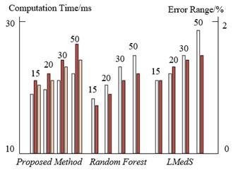
Figure 5. Comparison of three algorithms in case of different load distances
Furthermore, this paper compares the performance of the proposed method, Random Forest, and LMedS algorithms at different distances through Figure 5, with the numbers above the bars indicating the approximate distance from the camera to the load. The dark red bars represent the error magnitude, the light red bars represent the error magnitude after adjusting the voxel size, and the white hollow bars show the changes in computation time. The results indicate that the errors of all algorithms are sensitive to the camera distance, with the error magnitude almost linearly increasing as the distance increases. However, the proposed method shows the most significant changes in error, particularly at greater distances, but by appropriately adjusting the voxel size, the error magnitude can be effectively reduced. Meanwhile, the proposed method exhibits strong stability in computation efficiency, with computation time showing almost no significant increase as the distance changes, still maintaining a certain efficiency advantage over the other algorithms. The experimental results suggest that the camera distance significantly impacts the error magnitude of the algorithms, with all algorithms showing increased errors as the distance increases. Although the error variation of the proposed method is larger, its advantage lies in effectively reducing the error through reasonable adjustment of the voxel size while maintaining the stability of computation efficiency. In contrast, while the Random Forest and LMedS algorithms show relatively stable error performance at certain distances, they do not demonstrate significant advantages in computation time.
The analysis results indicate that although the Random Forest algorithm can effectively reduce noise interference and improve recognition accuracy, its dependency on the number of threshold iterations requires further optimization to maintain efficiency and accuracy in different scenarios. The LMedS algorithm, although strong in anti-interference capability under complex models, has higher computational complexity, resulting in lower efficiency in practical applications. The proposed method demonstrates excellent computational efficiency, but due to the insufficient adaptability of voxel size selection, the error varies under different conditions. Therefore, to further improve system performance, future improvement directions should focus on enhancing the adaptability of voxel size selection to better control errors under different load volumes and measurement conditions while maintaining efficient computation speed.
The research content of this paper focuses on the real-time load monitoring of logistics delivery vehicles, mainly including three aspects of innovative work. First, a sub-pixel edge positioning method for 2D images is proposed to improve the accuracy of load recognition. Second, the fitting interpolation technique between continuous image frames is studied to enhance the continuity and consistency of image data. Finally, a real-time load volume calculation method based on image data analysis and processing is proposed. The combination of these technologies aims to improve the real-time monitoring capabilities of the logistics delivery system, providing technical support for efficient and accurate load management. Experimental results show that the proposed method significantly improves recognition accuracy after sub-pixel edge positioning for 2D images, but the error magnitude fluctuates under different load volume and load distance combinations. This fluctuation is mainly related to the insufficient adaptability of voxel size selection. Additionally, the proposed method performs stably under different load distances, maintaining high computation speed, but compared with Random Forest and LMedS algorithms, the error magnitude shows slight fluctuations in some scenarios. Nonetheless, the proposed method still has advantages in overall performance, especially in scenarios with large load volumes or long load distances, demonstrating strong adaptability and computational efficiency.
Overall, the research results of this paper have significant value in improving the accuracy and efficiency of load monitoring for logistics delivery vehicles, especially in application scenarios requiring real-time monitoring and rapid computation. However, the study also has some limitations, mainly in the adaptability of voxel size selection and error control. Future research directions should focus on further optimizing the adaptive algorithm for voxel size selection to better adapt to different load conditions, reduce error magnitude, and improve the overall robustness and accuracy of the system while maintaining efficient computation.
[1] Tan, K.M., Ramachandaramurthy, V.K., Yong, J.Y., Padmanaban, S., Mihet-Popa, L., Blaabjerg, F. (2017). Minimization of load variance in power grids—investigation on optimal vehicle-to-grid scheduling. Energies, 10(11): 1880. https://doi.org/10.3390/en10111880
[2] Pinkney, B., Dagenais, M.A., Wight, G. (2022). Dynamic load testing of a modular truss bridge using military vehicles. Engineering Structures, 254: 113822. https://doi.org/10.1016/j.engstruct.2021.113822
[3] Deng, M., Wang, L., Zhang, J., Wang, R., Yan, Y. (2017). Probabilistic model of bridge vehicle loads in port area based on in-situ load testing. In IOP Conference Series: Earth and Environmental Science, 94(1): 012205. https://doi.org/10.1088/1755-1315/94/1/012205
[4] Yuen, K.V., Guo, H.Z., Mu, H.Q. (2023). Bayesian vehicle load estimation, vehicle position tracking, and structural identification for bridges with strain measurement. Structural Control and Health Monitoring, 2023(1): 4752776. https://doi.org/10.1155/2023/4752776
[5] Shokravi, H., Shokravi, H., Bakhary, N., Heidarrezaei, M., Rahimian Koloor, S.S., Petrů, M. (2020). Vehicle-assisted techniques for health monitoring of bridges. Sensors, 20(12): 3460. https://doi.org/10.3390/s20123460
[6] Laxman, K.C., Ross, A., Ai, L., Henderson, A., Elbatanouny, E., Bayat, M., Ziehl, P. (2023). Determination of vehicle loads on bridges by acoustic emission and an improved ensemble artificial neural network. Construction and Building Materials, 364: 129844. https://doi.org/10.1016/j.conbuildmat.2022.129844
[7] Kale, U., Rohács, J., Rohács, D. (2020). Operators’ load monitoring and management. Sensors, 20(17): 4665. https://doi.org/10.3390/s20174665
[8] Silva, A., Sánchez, J.R., Lozoya-Santos, J.D. (2019). Comparative analysis in indirect tire pressure monitoring systems in vehicles. In 9th IFAC International Symposium on Advances in Automotive Control (AAC). IFAC PapersOnLine, 52(5): 54-59. https://doi.org/10.1016/j.ifacol.2019.09.009
[9] Lydon, D., Taylor, S., Lydon, M., del Rincon, J.M., Hester, D. (2019). Development and testing of a composite system for bridge health monitoring utilising computer vision and deep learning. Smart Structures and Systems, 24(6): 723-732. https://doi.org/10.12989/sss.2019.24.6.723
[10] Pham, V.T., Son, H.S., Kim, C.H., Jang, Y., Kim, S.E. (2023). A novel method for vehicle load detection in cable-stayed bridge using graph neural network. Steel and Composite Structures, 46(6): 731-744. https://doi.org/10.12989/scs.2023.46.6.731
[11] Roy, A., Mukherjee, P.S. (2024). A control chart for monitoring images using jump location curves. Quality Engineering, 36(2): 439-452. https://doi.org/10.1080/08982112.2023.2232441
[12] Trigub, M.V., Vasnev, N.A., Kitler, V.D., Evtushenko, G.S. (2021). The use of a bistatic laser monitor for high-speed imaging of combustion processes. Atmospheric and Oceanic Optics, 34(2): 154-159. https://doi.org/10.1134/S102485602102010X
[13] Bekeneva, Y.A., Petukhov, V.D., Frantsisko, O.Y. (2020). Local image processing in distributed monitoring system. Journal of Physics: Conference Series, 1679(3): 032048. https://doi.org/10.1088/1742-6596/1679/3/032048
[14] Sundaram, N., Meena, S.D. (2023). Integrated animal monitoring system with animal detection and classification capabilities: A review on image modality, techniques, applications, and challenges. Artificial Intelligence Review, 56(Suppl 1): 1-51. https://doi.org/10.1007/s10462-023-10534-z
[15] Kim, D.H., Seely, N.K., Jung, J.H. (2017). Do you prefer, Pinterest or Instagram? The role of image-sharing SNSs and self-monitoring in enhancing ad effectiveness. Computers in Human Behavior, 70: 535-543. https://doi.org/10.1016/j.chb.2017.01.022
[16] Lay-Ekuakille, A., Telesca, V., Giorgio, G.A. (2019). A sensing and monitoring system for hydrodynamic flow based on imaging and ultrasound. Sensors, 19(6): 1347. https://doi.org/10.3390/s19061347
[17] Terada, I., Togoe, Y., Teratoko, T., Ueno, T., Ishizu, K., Fujii, Y., Shiina, T., Sugimoto, N. (2020). Monitoring of portal vein by three-dimensional ultrasound image tracking and registration: Toward hands-free monitoring of internal organs. Advanced Biomedical Engineering, 9: 1-9. https://doi.org/10.14326/abe.9.1
[18] Kong, B., Yu, M., Ye, S., Xu, X., Xiang, R. (2023). Design of eutrophication monitoring platform for Chaohu connected river channel based on LoRa and deep learning. UPB Scientific Bulletin, Series C, 85(3): 285-296.
[19] Chen, J., Zhang, D., Yang, S., Nanehkaran, Y.A. (2020). Intelligent monitoring method of water quality based on image processing and RVFL-GMDH model. IET Image Processing, 14(17): 4646-4656. https://doi.org/10.1049/iet-ipr.2020.0254
[20] Fauzi, R., Suherman, Maulana, R. (2017). Designing and characterizing periodic image monitoring device for remote surveillance purpose. Journal of Physics: Conference Series, 801(1): 012082. https://doi.org/10.1088/1742-6596/801/1/012082
[21] Walterscheid, I., Biallawons, O., Berens, P. (2019). Contactless respiration and heartbeat monitoring of multiple people using a 2-D imaging radar. In 2019 41st Annual International Conference of the IEEE Engineering in Medicine and Biology Society (EMBC), Berlin, Germany, pp. 3720-3725. https://doi.org/10.1109/EMBC.2019.8856974