Vasudevan Narasimman*![]() | Karthick Thiyagarajan
| Karthick Thiyagarajan![]()
© 2023 IIETA. This article is published by IIETA and is licensed under the CC BY 4.0 license (http://creativecommons.org/licenses/by/4.0/).
OPEN ACCESS
The ability to accurately and swiftly detect grape leaf diseases is paramount in preventing and managing grapevine afflictions. A delay in the identification and treatment of these infections can lead to substantial economic losses owing to reduced grape yields and compromised quality. Conventional deep learning models, such as ResNeXt and Capsule Networks, though effective, are resource-intensive and require extensive training time. Their application on resource-constrained devices or in remote vineyards can, therefore, be challenging. Capsule Networks hold significant promise in grape leaf disease identification due to their ability to preserve hierarchical relationships and spatial hierarchies of grape leaves. This study presents an innovative approach to grape leaf disease detection by constructing a lightweight Capsule Network that utilizes depth-wise separable convolutions. This modification from traditional convolutions, used in ResNeXt and conventional Capsule Networks, enhances the reception of the convolution field and facilitates the extraction of deep-level features from infected leaf images, while minimizing computational cost and improving training results. A comprehensive disease severity index, calculated from the entirety of the leaf images, is incorporated to assess the stages of plant disease by considering all leaf infections. Experimental results obtained from the Plant Village public dataset demonstrate the efficacy of the proposed method in diagnosing grape leaf diseases. The method exhibits a marked reduction in computational complexity compared to the existing deep learning model, ResNeXt, and traditional Capsule Neural Networks. In addition to disease detection, the severity index also allows for quantifying the stage of the disease. The findings of this study underscore the potential of the proposed depth-wise separable convolution-based lightweight Capsule Network in facilitating efficient and comprehensive grape leaf disease detection and assessment.
imaging, separable convolution, disease recognition, neural network, and classification
Convolutional Neural Networks (CNNs) possess the ability to recognize features irrespective of their position in an image due to their property of translation invariance. However, they can grapple with complex transformations that extend beyond fundamental translations. Capsule Neural Networks (CapsNets), with their ability to capture hierarchical spatial relationships, could potentially address more intricate changes associated with grape leaf diseases. While pooling layers in CNNs extract hierarchical features, they may inadvertently lose information. In contrast, CapsNets inherently manage hierarchical characteristics by design, which could be beneficial for diseases with complex structures in grape leaves.
Capsule Neural Networks, a distinct form of neural network architecture, are designed to better manage the spatial and hierarchical relations among features in images or other types of data [1, 2]. Each layer in a CapsNet contains multiple "capsules" or groups of neurons that represent varied visual aspects or attributes of the input data. The interaction between these capsules forms a hierarchical representation of the data. The primary innovation in CapsNet is the implementation of "dynamic routing," which allows capsules in one layer to interact preferentially with capsules in the following layer, based on their prediction consensus [3]. This direct representation of feature relationships by CapsNets helps overcome some limitations of traditional CNNs. CapsNet shows promise in enhancing the robustness and interpretability of deep learning networks, particularly for image and video data. Despite being a relatively new field of study, it is anticipated that more advancements and modifications are on the horizon.
A capsule network is primarily composed of two essential components: encoders and decoders [4, 5]. With a total of six layers, the first three layers constitute the encoder, responsible for transforming the input image into a vector. The initial layer of the encoder, a convolutional neural network, extracts the fundamental features of the image. The second layer, the PrimaryCaps Network, uses these basic elements to discern more complex patterns. The third layer, the DigitCaps Network, comprises a variable number of capsules. After these stages, the encoder produces a vector that proceeds to the decoder. The decoder, consisting of three interconnected layers, uses this vector as a starting point to attempt to reconstruct the original image. This ability to predict events based on its experience strengthens the network.
The matrix between the first layer and the second layer is multiplied to encode spatial relationship information, and the encoded information represents the probability of label classifications. During the computation step, the lower-level capsules adjust their weights in accordance with the weights of the higher-level capsules. They do this to align with the weights of the superior capsules. The higher-level capsules map the weight distribution and permit the majority to pass. Through dynamic routing, they can all communicate with each other. During dynamic routing, the lower capsules transmit their data to the parent capsule. The capsule that receives the majority of data is designated as the parent capsule. All capsules send their data to the capsule they deem most appropriate. The parent capsules distribute the weights according to the agreement.
Dynamic routing can encounter difficulties when identifying disease spots on grape leaves when these images are presented as input. The capsules focus their attention on the image, particularly its invariant aspects, aligning the frame of the leaf with respect to its borders. After determining whether the object is a leaf, they relay their predictions to the higher-level capsules. If the projections of the leaf's edges correspond with the predictions of other lower-level capsules, the object is classified as a leaf. This process exemplifies routing by agreement.
Dynamic routing plays a crucial role in Capsule Neural Networks by orchestrating how lower-level information is amalgamated to form higher-level features. Initially, the input image of the grape leaf is processed through convolutional layers to identify basic attributes, such as edges and corners. Each discerned feature prompts the activation of a primary capsule. The activation vector linked to a primary capsule denotes the properties of the specified feature, including aspects like orientation, location, and various visual qualities. For each primary capsule, a transformation matrix is obtained.
This matrix embodies a means of encoding how lower-level features transform to contribute to the formation of higher-level features. The transformation matrix symbolizes the relationships between the activations of primary capsules and their collective representation of more complex patterns. Prediction vectors in higher-level capsules are formulated by calculating the weighted sum of primary capsule activations, which are then transformed using their respective transformation matrices. These prediction vectors denote the existence and attributes of features on a higher level. Within the scope of grape leaf disease identification, these characteristics could correspond to different disease symptoms or patterns.
Following the generation of transformation matrices and prediction vectors, the initialization of routing weights is performed. This involves assigning initial values to the routing weights that connect primary and higher-level capsules, a process known as weight initialization. The routing weights dictate the degree to which primary capsules contribute to the prediction vectors of higher-level capsules.
During each iteration of dynamic routing, the following steps occur:
Prediction Aggregation: The transformation matrices of primary capsules are multiplied by activations to generate "transformed prediction vectors". These transformed vectors from all primary capsules are then summed to feed into higher-level capsules.
Routing Update: A softmax operation is applied to the input to yield routing weights that represent the agreement between primary and higher-level capsules. These routing weights determine the extent to which each primary capsule's information impacts the prediction vectors of higher-level capsules.
Weighted Sum: The weighted contributions of primary capsules are combined to form the output prediction vectors of higher-level capsules.
The final layer of the CapsNet comprises output capsules, each representing a distinct illness category or pattern. The prediction vectors produced by these output capsules are based on the inputs from higher-level capsules, with each prediction vector being unique to a specific class.
Capsule neural networks address the limitations associated with spatial and hierarchical relationships between features in traditional convolutional neural networks [6, 7]. However, CapsNets also present challenges and constraints, including high computational cost and the need for more scalability [8]. Due to their increased processing demands, training and predicting with CapsNets may be challenging for devices with limited resources [9, 10]. Additionally, the cost and complexity of computation can escalate significantly when more layers and capsules are added, making CapsNets difficult to scale.
To address these drawbacks, a new advancement called lightweight capsule neural networks (LWCNs) has been introduced [11]. LWCNs aim to reduce the computational cost and training time associated with CapsNets. Compared to CapsNets, LWCNs offer several benefits:
Reduced Computational Cost: LWCNs are designed to be compact and efficient, making them suitable for deployment on resource-constrained devices, including smartphones and embedded systems.
Improved Scalability: Depending on the complexity of the task and the available resources, LWCNs can be scaled up or down.
Enhanced Performance: LWCNs have shown promising results in various computer vision applications, such as object recognition and image classification, sometimes outperforming traditional CNNs and CapsNets.
A variant of CapsNet, known as a lightweight capsule neural network (LWCN), has been developed to be computationally efficient and suitable for deployment on systems with limited computing resources, such as mobile devices, IoT devices, and embedded devices [12]. The primary goal of a lightweight CapsNet is to reduce the number of input parameters and computations while maintaining high accuracy. Several strategies are employed to achieve this, including compression, pruning, quantization, factorization, and knowledge distillation. Compression involves reducing the number of capsules, neurons, and convolutional filters in each layer to minimize the number of parameters [13]. Pruning involves removing redundant connections or neurons that do not significantly contribute to the output. Quantization involves representing weights and activations with lower precision to conserve memory and accelerate inference. Factorization techniques like low-rank approximation are used to minimize the number of parameters in convolutional layers [14]. Knowledge distillation involves training the smaller network to mimic the larger one, thereby transferring knowledge from a larger CapsNet to a smaller one.
The task of identifying grape leaf diseases using deep learning models, including capsule neural networks, presents several challenges, such as imbalanced datasets, fine-grained discrimination, complexity, and CPU resources. For effective learning, deep learning models require a large and well-balanced dataset. If the dataset is limited in size or exhibits uneven distribution across various disease classifications, the model might struggle to effectively adapt to new, unseen data.
Grape diseases often cause subtle changes in the texture, color, and structure of leaves. To distinguish between different disease categories, deep learning models need to capture this fine-grained information. Standard convolutional neural networks might struggle with this task unless they are sufficiently complex and deep.
Deep learning models like ResneXt [15] and Capsule networks demand substantial computational resources for training and inference processes. Limited access to powerful hardware can pose a challenge for researchers. Additionally, detecting disease on a single leaf doesn't provide a comprehensive picture of the overall health of the grape plant. Therefore, this study focuses on determining the disease severity index to assess the overall disease status and to identify whether the diseases are in their initial or advanced stages.
The aforementioned issues with existing grape leaf disease detection systems have led to the proposal of a new network called lightweight capsule networks. The main contributions of this paper are:
Before sending features to the capsule layers for spatial relationship analysis, extracting features from an input picture using depth-wise convolution as part of a capsule network design is feasible. While it provides more effective and lightweight computing, depth-wise convolution is generally utilized in this context to replace classic convolutional layers. Unlike standard convolutional layers, which apply each filter to every input data channel simultaneously, depth-wise convolution applies each filter to just one channel simultaneously. This makes the model more effective by lowering the number of parameters that must be learned. Combining depth-wise convolution with capsule networks may produce an efficient and effective lightweight capsule neural network model for picture object recognition. The following capsule layers investigate the spatial correlations between the low-level data extracted by the depth-wise convolutional layer to recognize objects in the picture.
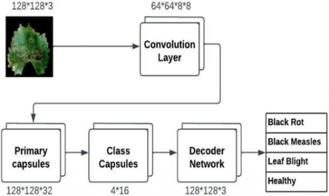
The classic CapsNet ideas used to determine the illness of grape leaves are shown in Figure 1. The input layer receives a picture with the dimensions 128×128×3. The convolutional layer performs a typical convolution to extract information from the input picture. Usually, a non-linear activation function like ReLU is present in this layer [16]. The number of filters or the convolution stride may be changed to alter the output size of this layer, which is typically less than the input size. The output of the convolutional layer is transformed into capsules by the main capsule layer. Each of these capsules, which are 16-dimensional vectors, is placed in an 8x8 grid. A tensor of the dimensions 8×8×256, where 256 is the number of capsules, is the output of the principal capsule layer [17]. The output from the primary capsules layer is subjected to dynamic routing in the digit capsules layer, enabling the capsules to exchange information and coordinate their outputs. The layer of digit capsules produces a tensor of size 4x16, where 4 is the number of classes, and 16 is the dimension of each output capsule.
The decoder network [18] recreates the input picture using the digit capsules layer's output. To do this, the output capsules are sent through several completely linked layers, each of which gradually converts the output capsules into a pixel-by-pixel image reconstruction. The decoder network produces a tensor with the dimensions 128×128×3, representing the reconstructed picture. To determine the class of the input picture, the output layer employs the results from the digit capsules layer. A softmax function is applied to the output capsules, and the class with the highest probability is chosen [19]. The likelihood that the input picture belongs to each of the four categories is contained in a tensor of dimension four produced by the output layer.
A tensor with the dimensions [batch size, height, width, channels] is the input to a CapsNet. The first layer of the network is commonly a convolutional layer that uses a kernel with the shape [kernel size, kernel size, channels, filters] to conduct conventional convolution on the input tensor. Filters are the number of output channels in this case. The convolutional layer is represented as:
$\mathrm{C}=\operatorname{conv}(\mathrm{X}, \mathrm{K})$ (1)
where, C is the output shape [batch_size, height', width', filters], X is the input shape [batch_size, height, width, channels], and K is the convolutional kernel of shape [kernel_size, kernel_size, channels, filters]
Convolutional layer output is transformed into a tensor of capsules by passing it via a non-linear activation function like ReLU. Assume that the convolutional layer's output is a tensor C with the following dimensions: batch size, height', width', and filters. It may be reshaped into a tensor P with the following dimensions: batch size, height * width * filters / caps_dim, caps _dim, where caps dim is the dimensionality of each capsule. The primary capsule layer is represented as:
$\mathrm{P}=$ reshape $($ activation $(\mathrm{C}))$ (2)
where, P is output tensor of shape [batch_size, height' * width' * filters / caps_dim, caps_dim], activation is an activation function, such as ReLU, and reshape is a reshape operation
In CapsNets, the output of the primary capsule layer is routed to the appropriate higher-level capsule based on the agreement between the output and the capsule's prediction vector. This is done by computing the scalar product between the output and the weights of each capsule, squashing the result using a non-linear activation function, and so on. The capsule operations can be represented as:
$u_{\text {hat }}=W @ P$ (3)
$\mathrm{u}=\mathrm{squash}\left(\mathrm{u}_{\mathrm{hat}}\right)$ (4)
$\mathrm{v}=$ route $(\mathrm{u}, \mathrm{b})$ (5)
where, uhat is predicted output shape [batch_size, num_capsules_i, num_capsules_j, dim_j, 1], W is weight matrix shape [num_capsules_i, num_capsules_j, dim_i, dim_j], and P is input tensor of shape [batch_size, height' * width' * filters / caps_dim, caps_dim].
Without depth-wise separable convolution, CapsNets employ conventional convolutional layers that apply several filters to the input picture to extract features before passing those data through several fully connected layers to generate predictions. Then, capsules indicate the existence or absence of a specific characteristic in a picture.
Figure 1. Traditional CapsNet
Contrarily, the suggested method, LWCNs with depth-wise separable convolution, employs a unique convolutional layer that divides spatial filtering and channel filtering tasks [20]. This layer consists of two steps: pointwise convolution, which combines the filtered channels, and depth-wise convolution, which filters each channel of the input picture separately. By using fewer parameters, this method speeds up calculation without sacrificing precision. Figure 2 depicts the suggested depth-wise light-weight capsule neural network.
Figure 2. Depth-wise light-weight capsule neural network
Initially, a 128×128×3-pixel picture is loaded into the input layer (where 3 is the number of color channels - red, green, and blue). Subsequently, a depth-wise separable convolution layer is applied to the input data [21, 22]. Combining depth-wise convolution, which uses a distinct filter for each input channel, with pointwise convolution [23], this convolutional layer is intended to be more computationally efficient than ordinary convolution [24] (which involves a 1×1 filter to combine the output of the depth-wise convolution across channels).
This layer generates a 128×128×32 feature map. The feature map is then processed through two additional depth-wise separable convolution layers, each having twice as many channels as the feature map's spatial dimensions. These layers produce feature maps, the first of which is a 64x64x64 feature map and the second a 32×32×128 feature map.
The primary capsule layer uses the output from the preceding layer. It transforms information into capsules, vectors representing an object's attributes in a picture, including its scale, orientation, and location. Each of these capsules, which are 16-dimensional vectors, is placed in an 8×8 grid. A tensor of the dimensions 8×8×256, where 256 is the number of capsules, is the output of the principal capsule layer. The class capsules layer uses the output from the primary capsules layer. The mechanism it uses, known as dynamic routing, enables the capsules to interact with one another and coordinate their outputs. The layer of digit capsules produces a tensor of size 4×16, where 4 is the number of classes, and 16 is the dimension of each output capsule.
The decoder network recreates the input picture using the class capsules layer's output. To do this, the output capsules are sent through several completely linked layers, each of which gradually converts the output capsules into a pixel-by-pixel image reconstruction. The decoder network produces a tensor with the dimensions 128×128×3, representing the reconstructed picture. To determine the class of the input picture, the output layer employs the results from the digit capsules layer. A softmax function is applied to the output capsules, and the class with the highest probability is chosen. The probability that the input picture belongs to each of the four categories is contained in a tensor of dimension four produced by the output layer.
The dynamic routing mechanism of LWCNs uses depthwise convolution and pointwise convolution to detect the features and relationships among the features with less trainable parameters. Those depthwise convolution and pointwise convolution are represented in Eq. (6) and Eq. (7). Convolution is carried out independently on each input channel when using depth-wise convolution. Assume we have a depth-wise K of shape [kernel size, kernel size, channels, depth multiplier] and an input tensor X of shape [batch size, height, width, channels]. Here, the hyperparameter depth multiplier regulates the output tensor's depth. The depthwise convolution operation is represented as:
$Y=$ depthwise $\operatorname{conv}(\mathrm{X}, \mathrm{K})$ (6)
where, Y is the output shape [batch_size, height, width, channels * depth_multiplier], X is the input shape [batch_size, height, width, channels], and K is a depthwise kernel of shape [kernel_size, kernel_size, channels, depth_multiplier]. With a 1x1 kernel, pointwise convolution entails applying convolution to the depthwise convolution's output. Suppose we have a pointwise kernel K with the shape [1, 1, channels * depth multiplier, filters] and an input tensor Y with the shape [batch size, height, width, channels * depth multiplier]. Filters are the number of output channels in this case. The pointwise convolution operation can be represented as:
$\mathrm{Z}=$ pointwise $\operatorname{conv}(\mathrm{Y}, \mathrm{K})$ (7)
where, Z is output shape [batch_size, height, width, filters], Y is input [batch_size, height, width, channels * depth_multiplier], and K is the pointwise kernel of shape [1, 1, channels * depth_multiplier, filters].
In LWCNs, the output of the pointwise convolution is routed to the appropriate higher-level capsule based on the agreement between the output and the capsule's prediction vector. This is done by computing the scalar product between each capsule's production and weights, squashing the result using a non-linear activation function, and so on. The capsule operations can be represented mathematically as:
$\mathrm{u}_{\text {hat }}=\mathrm{W} @ \mathrm{Z}$ (8)
$\mathrm{u}=\operatorname{squash}\left(\mathrm{u}_{\text {hat }}\right)$ (9)
$\mathrm{v}=$ route $(\mathrm{u}, \mathrm{b})$ (10)
where, uhat is predicted output of shape [batch_size, num_capsules_i, num_capsules_j, dim_j, 1], W is weight matrix of shape [num_capsules_i, num_capsules_j, dim_i, dim_j], and Z is input tensor of shape [batch_size, height, width, filters].
3.1 Depthwise light-weight capsule neural network Algorithm
Input: Original Grape Leaf Images D
Output: DT, BS, ES, and DS
Where DT denotes Disease Type,
DS denotes Disease Stage,
BS denotes the Beginning Stage,
ES denotes End Stage
Step1: Start
Step2: Apply depthwise convolution layers over the Images
Step3: Extract the Basic Features from images and form them
as primary capsules SC, LC, and YP
Where SC denotes a Small circle
LC denotes a Large circle
YP denotes Yellow Patches
Step4: Process the spatial information of basic features
Step5: Based on the frequency and spatial information of
capsules, find the overall features of DT
Step6: Repeat step2 to step5 for all grape leaf images
Step7: Calculate the disease severity index (DSI) by the
Following the formula to find the DS
DSI = Number of diseased leaves / Total number of
leaves * 100
Step8: If DSI < 30 then
return BS
else
return ES
Step9: End
The grape plant leaf disease detection algorithm using a depth-wise lightweight capsule neural network is given above. It shows how the disease types and stages are identified. Neuronal clusters called capsules hold information about the location, frequency, and possibility of an object being there. Each entity in an image has a capsule in a network of capsules that offers the probability that the entity exists as well as the spatial characteristics of that entity. Local entity features, such as tiny circles, large circles, and yellow patches, are discovered using the depth-wise convolution layers. The capsule layer gathers the overall feature illness kind using low-level feature frequency and spatial data. Eq. (11) calculates the Disease Severity Index [25, 26], which gives the idea about the infection stage [27] of the overall grape plant.
DSI $=\frac{\text { Number of diseased leaves }}{\text { Total number of leaves }} * 100$ (11)
The experimental setup and results of the traditional capsule neural network, deep learning model, and depth-wise light-weight capsule neural network are discussed in the following section.
The machine with the 2.90 GHz processor, 12 GB RAM Memory, and 4 GB Nvidia GeForce GTX 1080Ti GPU card implements the suggested approach for depth-wise lightweight capsule network-based grape leaves disease detection and classification. The system above does all of the computations. Concerning testing accuracy, epochs range from 30 to 50. The learning rate ranges between 0.01 and 0.001. To accommodate the network in the GPU, several batch sizes are tested. The range of the batch size is 5 to 32. It is set to 32 to accommodate computer memory. Several training parameter volumes are considered in the dataset throughout the training process [28]. Tables 1 and 2 include the ideal set of hyper-parameters [29, 30] for the ResNeXt model, conventional CapsNet model, and depth-wise lightweight-based CapsNet. The ResNeXt model uses the same hyperparameter values used for the classical CapsNet for batch sizes, epochs, learning rate, optimizer, and activation.
Table 1. Hyper-parameter of ResNeXt and traditional capsule network
|
Hyper-Parameter |
Value |
|
Convolution output channels |
32 |
|
Primary capsule convolution output channels |
32 |
|
Primary capsule vector length |
8 |
|
Class capsule vector length |
16 |
|
Class capsule output classes |
4 |
|
Reconstruction loss weight |
0.0005 |
|
Activation |
ReLu |
|
Optimizer |
Adam |
|
Learning rate |
0.001 |
|
Batch size |
32 |
|
Number of epochs |
50 |
Table 2. Hyper-parameter of depth-wise lightweight capsule network
|
Hyper-Parameter |
Value |
|
Depthwise separable convolution output channels |
32 |
|
Primary capsule convolution output channels |
256 |
|
Primary capsule vector length |
16 |
|
Class capsule vector length |
16 |
|
Class capsule output classes |
4 |
|
Reconstruction loss weight |
0.0005 |
|
Activation |
ReLu |
|
Optimizer |
Adam |
|
Learning rate |
0.001 |
|
Batch size |
32 |
|
Number of epochs |
50 |
The grape leaf image dataset includes images from the public PlantVillage dataset [31]. We used 12,000 grape leaf images of four different types from this data set. The different types of leaves used in this experiment are black rot, black measles, leaf blight, and healthy leaves.
The dataset is randomly divided into a training set and a test set, in which the training set is used for training parameters, and the test set is used to verify the model. The data distribution of all the four classes is shown in Table 3.
Table 3. The dataset used for CapsNet-based grape leaf disease classification
|
Class |
Total |
|
Black Rot |
3000 |
|
Black Measles |
3000 |
|
Leaf Blight |
3000 |
|
Healthy |
3000 |
|
Total |
12000 |
The depth-wise light-weight CapsNet model's accuracy for grape plant leaf infection is determined to be 95.04% based on the confusion matrix shown in Figure 3. The confusion matrix shows the success of the suggested technique for each class. This makes it possible to evaluate the classifier's effectiveness visually. Although the rows decide the output class, the columns provide the actual class. In contrast to diagonal cells, which indicate misclassified observations, non-diagonal cells reflect correctly classified data. The results were calculated and presented as a percentage using the suggested methodology and the test data. It is evident from Figure 4 and Figure 5 that all classes are identified using the ResNeXt model and the conventional capsNet model but with additional trainable parameters. As per Table 4, The ResNeXt model accuracy is less than the other two CapsNets Models. Also, All the metrics like precision, recall, f1-score, and accuracy show that there is only a very slight difference between the recommended depth-wise light-weight capsule neural network classification accuracy and traditional capsule neural network classification accuracy but with significant differences in trainable parameters.
Table 5 displays the training time and trainable parameters for all three models. Traditional CapsNet took more training time than ResNeXt and LWCN as the trainable parameters of CapsNet are very high compared to others. We used the convolution layer in the ResNeXt and conventional CapsNet model with 50 epochs. Nevertheless, we employed depth-wise separable convolution layers with 50 epochs in the second lightweight CapsNet model. Both depth-wise convolution and pointwise convolution are used in the depth-wise convolution layers. Pointwise convolution combines the filtered channels after depth-wise convolution applies a different filter to each channel of the input picture. By using fewer parameters, this method speeds up calculation without sacrificing precision. As a result, the depth-wise lightweight CapsNet has 90% fewer trainable parameters and training time than the original CapsNet model. The traditional first CapsNet model's total trainable parameters were 558,761,188, ResNeXt's total parameters were 257,864,288, and the depth-wise lightweight CapsNet model's total parameters were 51,092,559.
The accuracy of the depth-wise lightweight CapsNet model with fewer trainable parameters was 95.04%, compared to 95.37% for the initial standard CapsNet model with more trainable parameters. Figure 6 to Figure 11 depict this accuracy accomplishment and trainable parameters using 50 epochs for all three models. Because there are fewer parameters and calculations, the depthwise lightweight CapsNet takes less time to train than the conventional CapsNet and ResNeXt. The 558,761,188 parameters of the traditional CapsNet were all trained. 51,092,559 parameters were trained out of the 51,093,519 parameters in the depth-wise lightweight CapsNet. Yet, there were only a few changes in the accuracy that both models provided. Compared to the conventional CapsNet and ResNeXt, the trainable parameters of depth-wise lightweight parameters are very low. It will shorten the computation time for the suggested technique.
Figure 3. Confusion matrix of depth wise light-weight CapsNet
Figure 4. Confusion matrix of traditional CapsNet
Figure 5. Confusion matrix of ResNeXt
Table 4. Performance evaluation
|
Model |
Precision |
Recall |
F1-Score |
Accuracy |
|
ResNeXt |
89.64 |
88.72 |
89.17 |
91.64 |
|
Traditional CapsNet |
93.78 |
92.78 |
93.27 |
95.375 |
|
Depthwise convolution-based lightweight CapsNet |
93.47 |
92.89 |
93.17 |
95.041 |
Table 5. Training time and trainable parameters comparison
|
Model |
Training Time |
Trainable Parameters |
|
ResNeXt |
4 Hours 23 Minutes |
257,864,288 |
|
Traditional CapsNet |
11 Hours 45 Minutes |
558,761,188 |
|
Depthwise convolution-based lightweight CapsNet |
2 Hours 11 Minutes |
51,092,559 |
Figure 6. ResNext performance
Figure 7. ResNeXt parameters
A non-linear activation function, a routing mechanism, and finally, a matrix multiplication operation is used by each capsule in a typical CapsNet to calculate the output of the capsule. The need for extra weights and a dynamic routing process increases the computational cost of this routing strategy. In contrast, the classic convolution procedure is divided into a depth-wise convolution and a pointwise convolution by the depth-wise lightweight CapsNet. Whereas the pointwise convolution mixes the outputs of the depth-wise convolution over all channels, the depth-wise convolution conducts a separate convolution for each channel in the input. The CapsNet needs fewer parameters and calculations as a result of this split. Since it utilizes different weight matrices for each channel in the input, the depth-wise separable CapsNet has explicitly fewer parameters than other types of neural networks. Also, since depth-wise convolution only convolves each channel with a smaller filter, lowering the overall calculations, the depth-wise lightweight CapsNet needs fewer computations.
Finally, the disease severity index was computed using LWCN disease classification performance for the whole leaves. The disease severity index is calculated by Eq. (11), which uses the number of diseased leaves and the total number of leaves. In this work, 9124 leaves got infected among the 12000 leaves. As more than 70% of leaves are affected, i.e., the disease severity index was found to be 76.04%, it is considered the end stage of the disease. If less than 30% of leaves were infected, the disease would have been considered a beginning stage. Calculating this disease severity index helps the farmer get an overall idea about their grape plant.
Figure 8. Traditional CapsNet performance
Figure 9. Traditional CapsNet parameters
Figure 10. Proposed model performance
Figure 11. Proposed model parameters
In this work, we suggest using depth-wise lightweight CapsNet instead of the standard architecture of capsule networks and ResNeXt. The advanced Capsule networks are then empirically compared to the conventional CapsNet and ResNeXt models. The findings demonstrate that the proposed depth-wise lightweight Capsule network significantly reduces the models' size. These overall parameters and training time were much less than the ResNeXt and conventional CapsNet. With much fewer parameters, depth-wise lightweight CapsNet performs on par with traditional capsule models in terms of accuracy. We also used the proposed capsule networks to find the disease severity index of grape leaves. In the future, the disease severity index calculation can be compared with other metrics to see the overall health of the grape plant. Also, the LCWNs can be used with other crops with real-time datasets.
[1] Pasunuri, N.R., Aruva, V., Ashutosh, V., Mukesh, G. (2023). Analysis of capsule networks to detect forged images and videos. International Journal of Scientific Research in Engineering and Management, 7(5): 1-12. https://doi.org/10.55041/IJSREM17495
[2] Altan, G. (2020). Performance evaluation of capsule networks for classification of plant leaf diseases. International Journal of Applied Mathematics Electronics and Computers, 8(3): 57-63. https://doi.org/10.18100/ijamec.797392
[3] Patrick, M., Adekoya, A., Ayidzoe, M., Baagyere, E. (2019). Capsule networks – A survey. Journal of King Saud University - Computer and Information Sciences, 34(1): 1295-1310. https://doi.org/10.1016/j.jksuci.2019.09.014
[4] Vasudevan, N., Karthck, T. (2023). A hybrid approach for plant disease detection using E-GAN and CapsNet. Computer Systems Science and Engineering, 46(3): 337-356. https://doi.org/10.32604/csse.2023.034242
[5] Pande, S., Chetty, M. (2019). Analysis of capsule network (capsnet) architectures and applications. Journal of Advanced Research in Dynamical and Control Systems, 10(10): 2765-2771.
[6] Steur, N., Schwenker, F. (2021). Next-generation neural networks: Capsule networks with routing-by-agreement for text classification. IEEE Access, 9: 125269-125299. https://doi.org/10.1109/ACCESS.2021.3110911
[7] Manogaran, U., Wong, Y., Ng, B. (2021). CapsNet vs. CNN: Analysis of the effects of varying feature spatial arrangement. Advances in Intelligent Systems and Computing, Springer, 1251. https://doi.org/10.1007/978-3-030-55187-2_1
[8] Kushal, M.U., Nikitha, S., Shashank, L.M., Partha, S.S., Maruthi, M.N. (2022). Literature survey of plant disease detection using CNN. International Journal for Research in Applied Science and Engineering Technology, 10(1): 4721-4724. https://doi.org/10.22214/ijraset.2022.43474
[9] Dong, Z., Lin, S. (2019). Research on image classification based on Capsnet. In IEEE 4th Advanced Information Technology, Electronic and Automation Control Conference (IAEAC), Chengdu, China, pp. 1023-1026. https://doi.org/10.1109/IAEAC47372.2019.8997743
[10] Zhang, B., Qian, J., Xijiong, X., Xin, Y., Dong, Y. (2021). CapsNet-based supervised hashing. Applied Intelligence, 51: 5912-5926. https://doi.org/10.1007/s10489-020-02180-7
[11] Shu, X., Li, J., Shi, L., Huang, S. (2023). RES-CapsNet: an improved capsule network for micro-expression recognition. Multimedia Systems, 29: 1593-1601. https://doi.org/10.1007/s00530-023-01068-z
[12] Wang, Z., Chen, C., Li, J., Wan, F., Wang, H. (2023). ST-CapsNet: Linking spatial and temporal attention with capsule network for P300 detection improvement. IEEE Transactions on Neural Systems and Rehabilitation Engineering: A Publication of the IEEE Engineering in Medicine and Biology Society, 1: 1-12. https://doi.org/10.1109/TNSRE.2023.3237319
[13] Janakiramaiah, B. Gadupudi, K., Prasad, L.V., Karuna, A., Krishna, M. (2021). Intelligent system for leaf disease detection using capsule networks for horticulture. Journal of Intelligent & Fuzzy Systems, 41(1): 1-17. https://doi.org/10.3233/JIFS-210593
[14] Zhang, Z., Xu, J., Liu, N., Wang, Y., Liang, Y. (2022). CapsNet-LDA: predicting lncRNA-disease associations using attention mechanism and capsule network based on multi-view data. Briefings in Bioinformatics, 24(1). https://doi.org/10.1093/bib/bbac531
[15] Yadav, D., Jalal, A.S., Garlapati, D., Hossain, K., Goyal, Ayush., Pant, G. (2020). Deep learning-based ResNeXt model in phycological studies for future. Algal Research, 50: 102018. https://doi.org/10.1016/j.algal.2020.102018
[16] Bai, Y. (2022). RELU-function and derived function review. In SHS Web of Conferences, 144: 02006. https://doi.org/10.1051/shsconf/202214402006
[17] Okwuashi, O., Ndehedehe, C., Olayinka-Dosunmu, D.N. (2022). Tensor partial least squares for hyperspectral image classification. Geocarto International, 37(27): 17487-17502. https://doi.org/10.1080/10106049.2022.2129833
[18] Kumar, S., Mahapatra, R., Kumar, P. (2022). Decoder Design for massive-MIMO systems using deep learning. IEEE Systems Journal, 16(4): 6614-6623. https://doi.org/10.1109/JSYST.2022.3191192.
[19] Zhao, J., Lian, Q.S. (2023). Multi-centers SoftMax reciprocal average precision loss for deep metric learning. Neural Computing and Applications, 35: 11989-11999. https://doi.org/10.1007/s00521-023-08334-1
[20] Jensen, T. (2022). Spatial resolution of airborne gravity estimates in Kalman filtering. Journal of Geodetic Science, 12: 185-194. https://doi.org/10.1515/jogs-2022-0143
[21] Ye, H., Zhu, X., Liu, C., Yang, L., Wang, A. (2022). Furniture image classification based on depthwise group over-parameterized convolution. Electronics, 11(23): 3889. https://doi.org/10.3390/electronics11233889
[22] Choi, J., Sim, H., Oh, S., Lee, S., Lee, J. (2022). MLogNet: A logarithmic quantization-based accelerator for depthwise separable convolution. IEEE Transactions on Computer-Aided Design of Integrated Circuits and Systems, 41(12): 5220-5231. https://doi.org/10.1109/TCAD.2022.3150249
[23] Xu, X., Ding, Y., Lv, Z., Li, Z., Renke, S. (2023). Optimized pointwise convolution operation by ghost blocks. Electronic Research Archive, 31(1): 3187-3199. https://doi.org/10.3934/era.2023161
[24] Macias, S. (2022). On pointwise smooth dendroids. Revista Integración, 40(2): 137-158. https://doi.org/10.18273/revint.v40n2-2022001
[25] Juliantika K., Alchemi, P., Saputra, J. (2022). Impact of pestalotiopsis leaf fall disease on leaf area index and rubber plant production. In IOP Conference Series: Earth and Environmental Science, 995: 012030. https://doi.org/10.1088/1755-1315/995/1/012030
[26] Patil, S., Shrikant, D., Bodhe, K. (2011). Leaf disease severity measurement using image processing. International Journal of Engineering and Technology, 3(5): 297-301.
[27] Zhu, Y., Lujan, P., Dura, S., Steiner, R., Zhang, J., Sanogo, S. (2019). Etiology of Alternaria leaf spot of cotton in Southern New Mexico, Plant Disease, 103(7). https://doi.org/10.1094/PDIS-08-18-1350-RE
[28] Bhattacharjee, R., Ghosh, D., Mazumder, A. (2021). A review on hyper-parameter optimization by deep learning experiments. Journal of Mathematical Sciences & Computational Mathematics, 2(1): 532-541. https://doi.org/10.15864/jmscm.2407
[29] Pareek, V., Chaudhury, S. (2021). Deep learning-based gas identification and quantification with auto-tuning of hyper-parameters. Soft Computing, 25(4): 14155-14170. https://doi.org/10.1007/s00500-021-06222-1
[30] Young, S., Rose, D., Karnowski, T., Lim, S., Patton, R. (2015). Optimizing deep learning hyper-parameters through an evolutionary algorithm. In International Conference for High-Performance Computing, Networking, Storage and Analysis, Texas, Austin. https://doi.org/10.1145/2834892.2834896
[31] Hughes, D., Salathe, M. (2015). An open-access repository of images on plant health to enable the development of mobile disease diagnostics through machine learning and crowdsourcing. arXiv:1511.08060. https://doi.org/10.48550/arXiv.1511.08060