Detection and Classification of Plant Stress Using Hybrid Deep Convolution Neural Networks: A Multi-Scale Vision Transformer Approach

India, a stronghold of agriculture, contributed 19.9% to the nation's economy, as reported in the GDP statistics for 2020-21. The burgeoning population, projected to reach 9.2 billion by 2050, necessitates a substantial increase in crop production for sustainable growth [1]. In this context, Phytopathology, the study of plant diseases, plays a pivotal role. It assists in quantifying and diagnosing plant stress, often gauged through visual assessment of plant tissues [2]. Importantly, pinpointing the causative agent behind plant growth abnormalities remains a challenging yet crucial endeavor [3].

Recently, the Convolutional Neural Network (CNN), a novel technological approach, has shown promise in identifying the severity of symptoms in apple leaves affected by black rot, with accuracy exceeding 90% [4]. Another innovative method, PD2SE-Net, a multi-tasking CAD system, was able to categorize plant disease and estimate severity on the PlantVillage dataset with remarkable accuracy - 91% for severity estimation and 98% for disease classification [5]. These advancements underscore the importance of accurate and rapid plant disease identification, as diseases significantly impact food production and grain yield [6]. The main focus of the research is to identify the correct disease that affects the crops and induce appropriate measures to reduce the spread of the infection from one plant to another [7].

With the rapid development of Artificial Intelligence, many fields opted to solve their issues by incorporating time and manpower, and accurate measures to take immediate action don’t contribute to these AI-based technologies among them, object identification and classification captured the cause of the abnormality but also enhancing the yields and thereby increasing the economy of the country which in turn relies on Agriculture [8]. Usually, the pathological differences that occur in a plant are reflected in its leaves, stem, root, shoot, and flowers and among them, leaves are more identical in showing the difference [9]. One of the major concerns is to identify plant diseases at the early stage as plants are prone to various illnesses at every stage of their life cycle [10]. The traditional methods for detecting plant illness over large geographical area requires more manual methods leading to huge loss and it is important to implement timely the limelight in which different AI methods are effectively used in achieving the best results in the field of agriculture and the work here focused on extracting the useful features from tomato plant leaves using Gabor and color based filters and radial basis function was used to detect the disease at the early stage with an accuracy of 90.37% [11]. With new advancements in Computer vision, Deep Learning methods in particular Convolution Neural Networks proved to project good work in many areas like face recognition, image formation, face detection, object tracking, and image classification, and with this improvement, many works used CNN for detection as well as classification of plant diseases [12]. The improvements in deep learning algorithms were remarked with the introduction of a CNN algorithm for its distinguishing capabilities to differentiate between a spatial and temporal relationship which is used for extracting useful features from the image which stores meaningful information [13]. Image feature extraction plays an important role. The CNNs use a specific operation called convolution to extract the local features from a raw image which minimizes the need for human intervention. Traditional Machine learning algorithms need a manual process to extract features like shape, texture, and colour and finally using AI-based algorithms like KNN, and SVM the features are reduced as in the case of cucumber and many other species [14]. Several CNN (Convolution neural networks) models are used to identify plant diseases for instance Mask-RCNN was used to detect fusarium head blight disease in wheat which attained an average accuracy of 92.01% [15]. Similarly, Resnet152, MobileNet, and Inception V3, models have attained an accuracy of 77.65%, 73.50%, and 75.59% [16].

Apart from plant diseases, plant stress both Biotic and Abiotic also has significant importance. A pertained VGG-16 model is used to identify Biotic and Abiotic stress from Paddy from the field images belonging to 12 different stresses which obtained an average accuracy of 92.89% [17]. Though CNNs are good at exploring the hidden features of the image they fail to project the positional information of relative features and this is because the interpretation of deeper layers is not done appropriately by the new layers and this can be resolved by increasing the number of filters, this creates a great increase in the computational cost. Despite having many advantages, the CNN models have a major drawback concerning the size of the kernel which leads to the loss of focus on the global information of an image [18]. Several architectural changes are suggested but the experts which gave a path for the introduction of the attention mechanism by replacing it with the convolution layer have shown commendable results [19]. Transformers are a standard paradigm of Natural Language Processing that uses an attention mechanism in the field of computer vision. Vision Transformers (ViT) is the first designed Transformer model to handle 2D images where the self-attention mechanism is used to collect the information from an image which is further broken down into non overlapping patches with size 16×16 with 49M parameters which focuses on the global information by resolving long-range dependencies without compromising the computational efficiency. Furthermore, the newly formed 2D token are flattened into 1D tokens using linear Projection and are fed onto the Encoder layer [20]. But, the main drawback of ViT is that it could not work with small datasets as it focuses on extraction of long-range dependency features than on local features and the Transformer model requires large amount of data for training [21]. Though ViT outperforms existing CNN models, just by increasing the layers doesn’t give better performance and requires more memory to deal with high resolution images [22]. Several modifications were applied to the Transformer models finally concluding that to extract both local and global information it is better to combine ViT with CNN where convolution operations are replaced with attention mechanism [23].

An attempt to reduce the overhead of computational cost of the transformers, a pyramid structure was introduced to reduce the feature dimensions. But the pyramid structure works well with dense prediction tasks whereas while dealing with Image classification a new horizon should be implemented [24]. Analysing multi scale features on vision transformers proved to have achieved satisfying results for video and image classification [25]. A new technique called cross attention with Vision Transformers (cross-ViT) has gained more attention in recent times [26]. In order to obtain best results, we developed a hybrid model that uses Deep Convolution Neural Network with Multi scale Vision Transformers along with cross Attention (MCViT) to attain perfect balance between local and global spectral features and for identification of plant illness and classification of diseases and stress. Due to the wide range of managerial implications in the agricultural sector, several advancements are done in accurately identifying the biotic stress in plants. Mainly for early detection, transformers models are used to identify the severity of stress at the earliest by proactively identifying the onset of the disease. By applying the real time monitoring mechanism, this approach helps the farmers in identifying the loss on point to protect the crop from further damage. By introducing transformer models, the scope for detecting the plant stress at a large scale becomes more flexible. Even in Precision farming to improve the sustainability of the production plant stress detection gives a detailed insight into the pattern and analysis of yield loss and it greatly helps the farmers to concentrate on the particular target for the prevention of wide spread of diseases using transformer models, farmers can mitigate the use of pesticides while combatting with the environmental abnormalities effectively. In the area of Research, plant stress detection and classification using transformer models generates data related to frequency of occurrence of diseases, pattern analysis of stress which contributes to the future research for disease control strategies by fostering innovations in agricultural sector. From the above stated managerial implications, we conclude that our research focuses mainly on how transformer models can work effectively in identifying the biotic stress plants. The analysis of leaf diseases relies heavily on feature extraction. We can identify the root of plant stress more precisely. Even though CNN does feature extraction on its own, it is limited in what it can do because it only extracts a small number of crucial features. As a result, we added CNN functionalities to our study on vision transformers. With the aid of deep convolutional neural networks (DCNN) and multi-scale vision transformers, our work attempts to extract both local and global features from plant leaves. This model focuses on attaining correlation between different scales with dual branches. The contributions of our work include:

1. Inclusion of Multi Scale Vision Transformer architecture where a multi scale dual branch is used to fuse features obtained from various scales.
2. A hybrid model that combines the DCNN with proposed MCViT to extract absolute features.
3. To classify the disease and estimate its severity.

This paper focuses on the summary of the related works in section 2. Section 3 focuses on the dataset used for our work and the methodology to carry out our research followed by results and discussion in section 4 and the work was summarized with conclusion in section 5.

3.1 Dataset overview

In the Proposed work we have compared the results with 3 datasets-PlantVillage, Plant Village Paddy, DiaMOS dataset (peer leaf).

3.1.1 PlantVillage dataset

The PlantVillage dataset is mainly used for multiclass classification of images and it contains 55,448 background-only images (61,486 in the enhanced version) that are divided into 39 classes cateogorizing the images into healthy and diseased. This dataset contains variety of images belonging to various species like cherry, apple, cornrasphberry, blueberry, grape, orange, potato, bell pepper, peach, soyabean, squash, strawberry, tomato altogether 14 species. In addition to this this dataset also contains 17 fungal disease images, diseases caused by bacteria, mold, virus and mites. The example images of Plant Village dataset are shown in Figure 1.

1.png

Figure 1. Plant stress images. (a) bacterial spot of tomato, (b) phosphorus deficiency in corn plants, and (c) corn fields having stalk rot

The tomato dataset is made up of RGB images with size 256×256 collected in a controlled setting, with each leaf centered on a continuous background (tabletop or black). It has a total of 15,892 images in 10 categories (normal, stress), under 10 different labels like training: 11,204 images, Validation: 3,092 images and Testing: 1,596 images. The corn dataset includes 18MP ground photographs captured with an 18MP camera, as well as RGB images of corn leaves in their natural habitat and pictures of noisy cornfields (3456×5184 or 5184×3456 image size generated). The region of interest (plant stress, marked with the occurrence in each case) is situated in the exact middle of the image. There are 8,911 images total in the dataset among 11 categories (10 stress and normal) (divides as training-6,232 images, Testing-886 and validation-1,793 images). From the 6 categories, five labeled as stress images and one category as normal. Total of 6,635 images altogether make up the dataset (divided as training-4,642 images, Testing-660 and Validation-1,335 images. Because the plant leaf center plays a crucial role the corn and soybean datasets, each image center is cropped (made square) to 345×345 (1/10 resolution). No cropping or size changes are made to the tomato image.

3.1.2 Paddy crop

One of the wide publicly available data sources is PlantVillage which constitutes a total of 54,306 images belonging to 26 classes of 14 species with 3355 specifically focusing on paddy leaves. Among them paddy leaves are represented by 3355 images which includes images of various categories like Brown spot (523 images), Hispa (565 images), Leaf blast (779 images) and remaining images in a total of 1488. The dataset is enriched using classical image augmentation techniques, resulting in 167,750 images. To ensure consistency and computational efficiency, the images are resized into a resolution of 256×256 pixels. The dataset is then divided into three groups as training, validation, and testing. This partitioning enables effective model training, parameter tuning, and unbiased evaluation of model performance.

3.1.3 DiaMOS plant

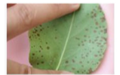
It is a real time dataset created, to identify and track plant ailments. Images of pear fruit with three different biotic stresses-primarily from leaves-are included in the DiaMOS plant dataset. In total, 3057 images were gathered, comprising both healthy and sick leaves that had experienced one or more biotic stressors, such as leaf spot, leaf desiccation, and slug damage as shown in Figure 2.

2.png

Figure 2. Sample of pear leaves stress images in DiaMOS plant dataset

3.2 Methodology

3.2.1 Data augmentation

Another crucial stage in computer vision is resizing the images before processing. By changing the size (width and height) of images it becomes easy for the model to train on newly preprocessed or scaled images. When compared to images, that are twice or three times larger than machine learning models can learn more quickly on tiny images since they don’t require the network to learn on as many pixels. When feeding the images into the Keras-based deep learning architecture pipeline, we used a technique to resize the images to 150×150 pixels and 224×224 pixels. There are two input sizes (150×150×3) and (224×224×3), where 150 and 224 are width and height and 3-way is a colour channel. Since samples of healthy plant leaves are significantly less than those of the other two types, we made a label-preserving alterations to plant leaves to fictitiously enhance the data/sample size and lessen model overfitting.

We followed the same with the images having same range with smaller pixel values to cut down the computing costs. This is done using a scale transformation. The parameter value (1/255) indicates that all pixel values fall between 0 and 1. To rotate an image by a specified angle, a transformation called rotation is applied. To randomly offset the image to the right or left, use the Width Offset Range transform and a value of 0.1 for the Width Offset parameter. By setting the Height Shift Range parameter to 0.1 can vertically shift the training images. The shearing angle is the angle at which the other axis is scaled up in a shearing transformation while the first axis is fixed to the image. In order to avoid this, a 0.2 shear angle is used. To conduct a random scaling transformation, the scaling range parameter is applied. Zooming in>1.0 on a picture requires a zoom factor of 0.2, whereas zooming out on an image requires a factor of<1.0. The image is turned horizontally with the flip apply function. A straightforward image processing technique generates 32,073 enhanced images, balancing the size of each class with images from the dataset of 2,000 images.

3.2.2 Elimination of natural background

In Pre-processing, segmentation plays a crucial role and is often considered as difficult operation. Before evaluating individual leaves, plant leaves must be segmented. The inclusion of depth information improves the accuracy of leaf segmentation process. Based on depth characteristics, backdrop plant leaves are first eliminated. However, the depth of the leaves is obviously different from that of the items in the backdrop. Since depth noise cannot be utilised to segment leaves, depth pictures of plant leaves are softer and cannot be represented. The depth of the leaf in mentioned in Figure 3.

3.png

Figure 3. RGB image of leaf depth

3.2.3 Enhanced mean-shift segmentation algorithm

Enhanced Mean-shift Segmentation techniques are used to estimate the local density gradients in correlation with image pixels as shown Figure 4. The process of gradient estimation is iteratively performed to identify similar pixels in corresponding images. It employs an enhanced mean-shift technique and segments images of object depth.

4.png

Figure 4. The proposed leaf segmentation method

The d-dimensional point set x_i=1 is the average motion vector at position x_i determined by n is given in Eq. (1):

$M(x)=\frac{\sum_{i=1}^n x_i K_W\left(x_i-x\right)}{\sum_{i=1}^n K_w\left(x_i-x\right)}-x$    (1)

where, the kernel function is represented in Eq. (2):

$K_w(x)=|W|^{-\frac{1}{2}} K\left(W^{-\frac{1}{2}} x\right)$       (2)

In practice, a diagonal matrix termed $\mathrm{W}$-add bandwidth matrix with positive symmetry-is utilized, with $\mathrm{x}$ designating the kernel's center. $x$ represents the position at which the vector in motion is caluclated. The average moving vector $\mathrm{M}(\mathrm{x})$ computes the local density gradient and the most significant direction of density increase for that pixel in improved average moving clustering. $x_i$ represents the $\mathrm{i}^{\text {th }}$ position in the $\mathrm{d}$ dimensional point set and $K_w\left(x_i-x\right)$ represents the difference between $x_i$ and $x$ applied to the kernel function $\mathrm{K}$. Summation $\Sigma$ is applied to values from 1 to n. From Eq. (2) the kernel function with parameter $\mathrm{w}$ is applied to $\mathrm{x}$ denoted by $K_w(x)$ and $|W|$ the determinant of matrix $W$ is calculated. $W^{-\frac{1}{2}} x$ represents the square root of inverse of $\mathrm{W}$ and kernel function $\mathrm{K}$ is applied to it. In order to find local density peaks, apply the formula given in Eq. (3):

$y_{j+1}=\frac{\sum_{i=1}^n x_i K_w\left(y_i-x_i\right)}{\sum_{i=1}^n K_w\left(y_i-x_i\right)}$      (3)

All points pointing to the apex that are plotted on the same peak are regarded as belonging to the same segment. This results in a general improvement in Mean Moving Segmentation.

Grayscale depth data are processed using a modified meanshifting clustering approach in this work to produce leaf areas and background. Let $x_i=1,2, \ldots, n$ represent the $2 \mathrm{D}$ input in the grayscale image space domain. The local density peak is represented by $y_{i, j}$ at pixel $x_i$ at iteration $j$. A more effective approach for shifting depth data segmentation is presented in the next section.

1. Creates the initial state of a window for coverage and a window for navigation in the radius ps and rs domains, respectively. A local density peak should be established at y_i, 1=x_i, iteration step j=1.
2. Depth difference for each pixel is calculated in the space window, distance window, and the centre pixel, then work out the motion vector of the navigation window.
3. Determine and set the average depth value y_iand average depth j+1 for each pixel in the spatial frame.
4. In the spatial window, clusters with cpp in range [1 ... m] are formed by pixels whose depth difference is less than the radius of the range window rs. Repeat the preceding methods until the shift values are modest enough to suggest convergence to determine whether the enhanced mean shifting clustering has reached convergence.

5.png

Figure 5. Enhanced mean shift segmentation of leaves, (a) mean-shift segmentation outcome, (b) segmentation results of the image depth and (c) RGB image segmentation view

Therefore, the depth picture is separated into sub-regions when mean-shift convergence takes place. These pieces are shown in different hues in Figure 5. By contrasting the RGB tones of green plant images with leaf images, Figure 5 demonstrates how the segmentation results are generated. In this stage, background items that are not green are eliminated. The plant picture is divided into several leaf images, which are then extracted from the segmented leaf depth and colour images.

In order to calculate a, use the GVF vector's four surrounding pixels, $p(i, j), p(i+1, j), p(i, j+1)$, and $p(i+1$, $j+1) . I$ and $j$ are the pixel coordinates of the image such that $v$ $(i, j)=x(i, j)$ and $y(i, j)$. for computing the pixel $p(i, j) \mathrm{GVF}$ vector for a given pixel. " $v$ " includes a function to indicate direction as in Eq. (4):

$\operatorname{sign}(x)=\left\{\begin{array}{c}1, x>0 \\ 0, x=0 \\ -1, x<0\end{array}\right.$   (4)

Therefore, the potential scattering point set s P is as follows mentioned in Eqs. (5)-(7):

$\begin{gathered}P_{s x}=\{p(i, j) \mid x(i, j) \leq x(i+ \\ 1, j) \text { and } \operatorname{abs}(\operatorname{sign}(x(i, j))+\operatorname{sign}(x(i+1, j))) \leq \\ 1\}\end{gathered}$     (5)

$\begin{gathered}P_{s y}=\{p(i, j) \mid y(i, j) \leq y(i+ \\ 1, j) \text { and } \operatorname{abs}(\operatorname{sign}(y(i, j))+\operatorname{sign}(y(i+1, j))) \leq \\ 1\}\end{gathered}$      (6)

$P_s=P_{s x} \cap P_{s y}$   (7)

where, $P_{s x}, P_{s y}$ represent the potential scattering points in the $\mathrm{x}$ and $\mathrm{y}$ direction. According to the center of divergence, the initialization of the contour model distinguishes lobes from occlusions. Each lobe's borders are shown by yellow lines, while the initialized model is shown by green circles in Figure 6.

6.png

Figure 6. Simulation results of plant stress segmentation

3.3 Proposed multi–scale vision transformer with DCNN

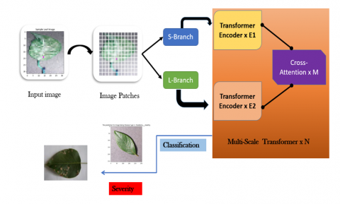
The input image is trimmed into patches of fixed size and constant scale for conventional Vision Transformers. Various cropping ratios are used for this process. Multi-scale feature representations of images are created for image recognition by dividing them into large and tiny chunks. Both tiny and large blocks can be used to represent little or huge patches, respectively, using small or large branches. This study employs two FCs to incorporate two branch outputs in turn, enabling the application of inputs obtained from two branches into the Vision Transformer. Figure 7 displays the class token and has an output dimension of 768. Dimension is utilized by each quadrant.

7.png

Figure 7. Architecture of proposed transformer with cross attention layer (CrossViT)

Normally, the Vision Transformer inputs the image tokens into multi-layer perceptron and the multi-head iterates them and the output is added to the token itself, and then again, the input is fed into the MLP, and multi-head layers iterate, and adds the output before that. Then, in the same way, repeat this process an additional L times before sending the result to the next transformer encoder. By simply repeating the embedding, this method does a poor job of shifting focus from the current input to the following layer. This cycle multiplies the attention of the next layer with the attention of the preceding layer to obtain new active attention. This technique allows for the effective utilization of the attention of every branch of Vision Transformer. The results of the following categorization efforts are improved by providing a piece of caution information. In Cross-Attention Fusion’s most recent two quarters, the class tokens are represented by the two circles above.

Our model is used to process large and small image patch tokens in two independent branches having different computational difficulties, and these image patch tokens are recurrently fused to complete one another. This project’s major objective is to create a classification system that works for visual translators. Using a cross-alert module that is effective, each transformer branch creates non-patch tokens to act as intermediaries for communicating information with other branches through attention. By merging CNN and ViT to add multi-scale capabilities rather than using a model that is only based on ViT, as in earlier work, our suggested method differs significantly from that of the prior research.

As an addition to the ResNet family of designs, the Non Local Network (NLN) is proposed. In this architecture, the last block includes a non-local aggregation procedure. Multi Head self-attention is connected to the ResNet bottleneck block using a Bottleneck Transformer introduced by the NLN design. These two techniques significantly enhance multi-vision work. Similar to how adding a CNN with non-local operations enhances image classification, we construct a DCNN and present it as CrossViT (DCNN-MCViT), which is a DCNN with ViT added, and use the DETR model for object recognition and picture activity. Contrary to earlier non-local block applications, we implement multi-scale interactions directly using our suggested DCNN-MCViT architecture by gradually adding CNNs.

Representations are typically transferred at low resolution levels in CNN-based image categorization networks. ResNet, for instance, has five stages with a final feature map that is 1/32×1/32 in each dimension. Each level reduces the resolution by half. ViT, on the other side, starts off with tokens that are 16×16 in size, which lowers the resolution in this dimension. At that resolution, the final layer yet persists. As a result, ViT has a higher likelihood of maintaining position data than ResNet. Since location information is not necessary for classification judgements in image classification tasks, we cannot claim that ViT has an advantage over ResNet since it keeps track of locations.

Due to the associations being explicitly embedded in the DCNN architecture, CrossViT typically needs a lot of training data to learn them. CrossFit can nonetheless discover intra-image correlations in the absence of these guided deflections. For example, capturing spatial rather than local semantics is impossible with DCNNs. To merge these two architectures, DCNN-MCViT uses CrossViT to compute non-local spatial semantics obtained from CNN to encode local data. The markers Tp from the obtained final feature map before the customary global pooling step are extracted to create the CNN feature map with kernel size P=1. Unlike the CrossFit model, which extracts labels directly from the input image X, this is not the case. We put forth a multi-scale hybrid visual transformer based on earlier jobs that join non-local activities with already-existing CNNs like CrossViT. Our suggestion is to apply CrossViT to the backbone CNN at various scales, as opposed to the original HViT which simply extended the backbone CNN with CrossViT. To translate the non-local spatial semantics of images to other scales, we additionally introduce cross-scale links between ViTs.

3.3.1 Cross-attention

Class tokens will be cautious while interacting with block tokens from larger branches of modules’ small branches in order to finally produce new class tokens. According to the architecture, in order to obtain a new class token for the large branch. To facilitate attention in the small branch, we perform a trade between the corresponding class token and the block token. This exchange ensures that the attention mechanism in the small branch focuses on the relevant information. Instead of directly using the class token, we substitute it with the block token, allowing the attention mechanism to consider the local context captured by the block token. This enables the small branch to concentrate on important features and enhance its attention-based operations.

Fusion should only be used on the minor branch. Then, as demonstrated in formula, project the minor branch’s class tokens via FC and compare the results to the major branch’s class token given in Eq. (8):

$x^{l s}=\left[f^s\left(x_{c l}^s\right) \| x_{\text {patch }}^l\right]$     (8)

where, the sub-branch class label is represented by $x_{c l}^s$ and $f^s$ is the FC used to project it to this dimension. Between class markers in the minor branch and block markers in the main branch, cross-annotation is performed throughout the entire module. The following formula can be used to numerically express cross attention following Eq. (9) and Eq. (10):

$q=x_{c l s}^{\prime s} W_q, k$    (9)

$A=\operatorname{softmax}\left(\frac{q k^T}{\sqrt{\frac{c}{h}}}\right)$     (10)

in which, C/h is the learnable parameter, C is the embedding dimension, and h is the total number of attention heads. The attention map produced by Cross-computational attentions and memory complexity is linear in our study because we only employ CLS tokens.

8.png

Figure 8. Cross-attention fusion sketch

Figure 8 illustrates the fundamental concept of our suggested intersectionality, wherein one quarter uses patch tokens and the other use Fusion CLS tokens. For example, to communicate information between patch tokens of various branches more quickly and efficiently, we first utilise the CLS tokens of each branch as a proxy before converting it into our own Backproject to the branch. The interaction between patch tokens in different forks helps contain information at various scales because the CLS token has learned abstract knowledge across all patch tokens in its own fork. The CLS token interacts with its own patch token in the following converter encoder after being fused with other branch tokens to amplify the information of each patch. The primary branch’s cross-attention module is described in the section that follows, and the operation is carried out by simply switching the secondary branch’s indexes l and s. The process of creating Attention maps in Cross-attention is more effective than All-Attention since we only employ CLS in the query, which reduces the computational and memory cost from quadratic to linear.

An input layer, one or more hidden layers that are switched sequentially from the input layer, and an output layer make up a multilayer neural network structure. A multilayer neural network contains many connections from the first layer to the network and vice versa. At this time, concentrate on the process’s closing steps for the greatest outcomes. In order to do this, a classifier with a softmax hierarchy is fed with a pooled set of the features that were determined in the previous stage. You may then decide which response is the most accurate using this. Unlike the activation function used in hidden layer, the output layer activation function is special. Each layer has a distinct function and execution strategy. After a classification procedure, the final hierarchy can produce class probabilities for incoming data as shown in Figure 9.

9.png

Figure 9. Proposed DCNN with CrossViT (DCNN-MCViT) with N multi scale transformer encoders having 2 inbuilt transformer encoders E1, E2 with a stack of M cross attention layers