Lijiao Zhang![]() | Jianzhen Wu
| Jianzhen Wu![]() | Jinxin Wei*
| Jinxin Wei*![]() | Xiaoyan Yu
| Xiaoyan Yu![]() | Jie Yu
| Jie Yu![]() | Bo Yuan
| Bo Yuan![]()
© 2023 IIETA. This article is published by IIETA and is licensed under the CC BY 4.0 license (http://creativecommons.org/licenses/by/4.0/).
OPEN ACCESS
Laboratory safety education is fundamental to the smooth conduct of scientific research. Traditional educational models are often limited in interactivity and real-time feedback and they struggle to satisfy the increasing needs of laboratory safety management. This study aims to enhance the interactivity and efficacy of laboratory safety education by adopting machine learning-enhanced image processing technologies. To cope with the noise issue in hazardous behavior data within laboratories, wavelet threshold denoising is applied to significantly improve data usability. To deal with the imbalance in data samples of laboratory hazard behaviors, an adaptive boundary data augmentation algorithm is introduced to balance the dataset and strengthen the model's generalization capability. A breakthrough in extracting spatio-temporal features of hazardous behaviors in laboratories is achieved through an improved Spatio-Temporal Graph Convolutional Network (ST-GCN) model, enabling effective recognition and classification of hazardous behaviors. The outcome attained in this study has important implications for enhancing the interactivity and practicality of laboratory safety education and it can expand new research directions for the application of machine learning in the field of image processing.
laboratory safety education, machine learning, image processing, wavelet threshold denoising, data augmentation, Spatio-Temporal Graph Convolutional Network (ST-GCN), hazardous behavior recognition
To cope with the frequent occurrences of laboratory safety incidents, effective laboratory safety education has become a particular important matter. Conventional methods of laboratory safety education often rely on text book or the instruction given by teachers, and they generally lack interactivity and real-time feedback [1-5]. Against this backdrop, machine learning-enhanced image processing technologies give us a new perspective for laboratory safety education. Real-time monitoring and analysis of hazardous behaviors in laboratories are carried out, making it possible to immediately identify potential safety risks, thereby enhancing the effectiveness and efficiency of safety education [6-8].
The great advancements in artificial intelligence in recent years have led to good achievements in image recognition and processing through machine learning. The application of these technologies has not only markedly improved the accuracy and speed of data processing but also enhanced the experience of interactive learning [9-13]. In case of laboratory safety education, the integration of machine learning and image processing techniques plays an important role, as it makes the effective identification and analysis of hazardous behaviors in laboratories possible, thereby providing learners with more intuitive and dynamic educational materials, which is of high theoretical and practical values [14-16].
However, existing studies about processing the data of laboratory hazard behaviors show some disadvantages, as the complex laboratory environments often results in noise-contaminated data of hazardous behaviors, and this can affect the accuracy of data analysis results [17-20]. Besides, the scarcity of certain types of hazardous behavior data can cause imbalance to datasets, potentially affecting the generalization capability and recognition effectiveness of the models, and these challenges would limit the application effect of machine learning methods in laboratory safety education [21-26].
To promote the application of machine learning techniques in laboratory safety education, this paper has three focuses. Firstly, the paper discusses the noise in hazardous behavior data from laboratories, and uses wavelet threshold denoising to pre-process the data, so as to effectively improving data quality. Secondly, to deal with data imbalance, an adaptive boundary data augmentation algorithm is applied to balance the dataset. Finally, by utilizing an improved ST-GCN model, spatio-temporal graphs of hazardous actions in laboratories are constructed, facilitating accurate extraction of spatio-temporal features and enabling efficient recognition and classification of hazardous behaviors. The in-depth exploration of these research aspects not only enhances the interactivity and efficacy of laboratory safety education but also provides new technical pathways and theoretical foundations for research in related fields, underscoring the significant value and application prospects of this study.
The core objective of laboratory safety education is to reduce the risk of accidents and ensure personnel safety. In this context, the use of machine learning-enhanced image processing technologies for hazardous behavior recognition not only facilitates real-time monitoring but also enables the prevention of potential safety hazards through historical data analysis. However, data preprocessing, particularly noise reduction, becomes a crucial step in ensuring the accuracy and reliability of machine learning models. The reasons and necessity for noise reduction in data are outlined below:
The primary reason is the complexity of laboratory environments, where noise is often introduced into the image and video data captured by monitoring devices due to various factors. Noise in the data can interfere with the training process of machine learning models, reducing their capability to recognize actual hazardous behaviors.
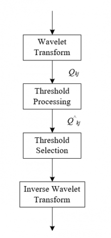
Wavelet threshold denoising is an effective technique for signal noise reduction. Initially, signals in the time domain are transformed to the wavelet domain using wavelet transform. This transform provides localized information in time and frequency, enabling better representation of signal characteristics in the wavelet domain. In this domain, noise and useful information within the signal are separated. Noise typically manifests as small amplitudes in the wavelet coefficients, while significant features of the signal correspond to larger coefficients. By setting an appropriate threshold, coefficients smaller than this threshold can be considered noise and suppressed, while those larger are retained.
Figure 1. Process flow of noise reduction in hazardous behavior data for laboratory safety education
The selection of a suitable wavelet threshold function is critical in ensuring effective noise reduction and preserving behavioral characteristics. Figure 1 gives the flow of noise reduction in hazardous behavior data for laboratory safety education. Wavelet threshold functions are categorized into hard and soft thresholds, each with distinct features and applicable scenarios. In hard thresholding, the treatment of wavelet coefficients follows a simple rule. A coefficient is retained if its absolute value exceeds the threshold; otherwise, it is set to zero. This means hard thresholding is an "all-ornothing" approach, potentially introducing sudden transitions in the denoised signal, which can cause additional distortion in certain scenarios. Soft thresholding is more subtle, not only zeroing coefficients below the threshold but also reducing those above it. Specifically, coefficients above the threshold are reduced by the threshold value; those below the negative threshold are increased by it, and if a coefficient's absolute value is at or below the threshold, it is set to zero. This method ensures smooth continuity at the threshold point, reducing signal distortion caused by hard thresholding but may also lead to some loss of signal detail. Assuming the estimated wavelet coefficients are denoted as $\hat{Q}_{k j}$, the decomposed wavelet coefficients as $Q_{k j}$, the sign function as $\operatorname{sgn}()$, and the threshold as $\eta$, the following expressions give formulas for hard and soft threshold functions:
$Q_{k j}=\left\{\begin{array}{l}Q_{k j},\left|Q_{k j}\right| \geq \eta \\ 0,\left|Q_{k j}\right|<\eta\end{array}\right.$ (1)
$\hat{Q}_{k j}=\left\{\begin{array}{l}\operatorname{sgn}\left(Q_{k j}\right)\left(Q_{k j}-\eta\right),\left|Q_{k j}\right| \geq \eta \\ 0,\left|Q_{k j}\right|<\eta\end{array}\right.$ (2)
In traditional wavelet threshold denoising methods, the determination of the threshold is often related to the root mean squared error (RMSE) of the wavelet coefficients and the number of sampling points. However, when applied to noise reduction in hazardous behavior data for laboratory safety education, this traditional method of threshold selection may not be suitable. The main reason is that laboratory safety monitoring often involves dynamic scenes, where hazardous behaviors are variable and complex. Traditional wavelet threshold methods may not adapt well to such dynamic changes, as they are typically designed for relatively static or steady-state noise. Also, the characteristics of hazardous behavior signals may vary with time, environmental conditions, and operational methods during the experiment. The threshold needs to be adaptable to these changes to ensure effective denoising. Assuming the RMSE of noise is represented by $\delta$, the number of signal sampling points by $B$, the decomposition scale by $k$, and the root mean squared error of the wavelet coefficients at the $k$-th level by $\delta_k$, the following equations provide the commonly used threshold expressions in traditional wavelet threshold denoising:
$\eta=\delta \sqrt{2 \ln B}$ (3)
$\eta_k=\delta_k \sqrt{2 \ln B} / \ln (k+1)$ (4)
Considering the specific needs of hazardous behavior recognition in laboratory safety education, this paper introduces an exponential function concept to improve the threshold function. With the form of an exponential function, the threshold becomes more sensitive to local features of the signal, allowing for adaptive threshold adjustment to better accommodate changes in signal characteristics. At the same time, it enables better preservation of signal details during denoising, especially those subtle features crucial in safety monitoring. Assuming the sign function is represented by sgn(Qkj), the expression is as follows:
$\hat{Q}_{k, j}=\left\{\begin{array}{l}\operatorname{sgn}\left(Q_{i j k}\right)\left(\left|Q_{k j}\right|-\left|Q_{k j}\right| \cdot r^{\eta-\left|Q_{k i}\right|}\right),\left|Q_{k j}\right| \geq \eta \\ 0,\left|Q_{k j}\right|<\eta\end{array}\right.$ (5)
From the above equation, it is clear that when $Q_{k j}>0$, the value is $m$, and when $Q_{k j}<0$, the value is -1 . When $\left|Q_{k, j}\right|=\eta$, $Q_{~~k j}^{\wedge}=0$, at this point the threshold function is continuous at $\left|Q_{k, j}\right|=\eta$, addressing the issue of discontinuities present in hard threshold functions. As $\mid Q_{k, j}$ approaches infinity, $Q_{~~k, j}^{\wedge}$ infinitely approaches $\left|Q_{k, j}\right|$, avoiding the issue of soft threshold functions compressing some wavelet coefficients with a fixed value. By appropriately selecting the wavelet function and threshold, the denoising process can remove noise while retaining as much as possible the key features of hazardous behavior, which is crucial for subsequent behavior recognition and assessment.
In the context of laboratory safety education, utilizing machine learning-enhanced image processing technologies to identify hazardous behaviors is a promising research direction. However, the training of machine learning models requires a large amount of data. If a dataset contains an too much of s certain category and too little of others, the model may become biased towards the category with more samples. Via the balancing treatment, the sample count of each category becomes equal, which enables the model to fairly learn the characteristics of each kind of the behavior, thereby enhancing the model’ ability in recognizing hazardous behaviors that are not that common.
This paper attempts to propose an adaptive boundary data augmentation algorithm for balancing hazardous behavior data of the laboratory safety education environment. Objective of this algorithm is to balance the dataset by creating different-type samples on the edge or boundary, so as to strengthen the model's ability to recognize hazardous behaviors of minority classes. At first, the algorithm identifies boundary samples in the dataset, such as those near the dividing line between different categories. In terms of laboratory safety education, these boundary samples may be the initial or atypical manifestations of some hazardous behaviors, and this step is crucial for training a model that can accurately identify various hazardous behaviors. After the boundary samples are identified, the algorithm creates new data points based on these samples. In this way, new variants between known categories are generated, enriching the dataset and helping the model learn to better differentiate between different types of behaviors. Besides generating random samples, the algorithm can do it adaptively based on the current performance of the model, and this means that if the model performs poorly on a particular category, the algorithm will prioritize generating more boundary samples for this category to enhance its recognition ability in that class. By adding newly generated boundary samples in categories with less samples, the algorithm can help balance the entire dataset, which is very important for training machine learning models as it prevents the model from being overly biased towards categories with more samples, in this way, it ensures a good recognition ability across all categories.
For hazardous behavior recognition in laboratory safety education, some behaviors might be relatively rare, but the importance of recognizing these behaviors can be very high. In such cases, ordinary data augmentation methods might not suffice to generate enough minority class samples to improve the model's performance. Therefore, an adaptive method is required to generate data more targetedly, and "sampling weight" is a part of this method. Assuming the sum of distances of a minority class sample to each of its k-nearest neighbors of the same class is represented by f1, the number of nearest neighbors in the sample set for any minority class sample is denoted by j1, and the number of nearest neighbors that are majority class samples is denoted by j2, the paper calculates the sampling weight q for minority class boundary samples through the following equation:
$q=j_1 * \frac{f_1}{j_1-j_2}$ (6)
The detailed steps of the adaptive boundary data augmentation algorithm are described as follows:
(1) In the context of laboratory safety education, hazardous behavior datasets often exhibit significant category imbalance. For example, behaviors like "non-compliance with procedures" or "failure to use personal protective equipment" might be less common, yet they are crucial to identify and prevent in safety education. To calculate the imbalance, first collect the sample numbers for each category of hazardous behavior, then determine the sample count for each category. After that, calculate the ratio of the smallest class sample size to the largest class sample size to determine the imbalance ratio. At last, assess the overall imbalance of the existing dataset. Assuming: the original training set is represented by $Y$, the minority set is represented by $B$, its sample count is represented by $b$, the majority set is represented by $L$, and its sample count is represented by $l$, the imbalance degree of the sample set $Y$ is represented by $\beta$, then its value can be calculated using this formula:
$\beta=\frac{l}{b}$ (7)
After determining the degree of imbalance, calculate how many new samples need to be synthesized for each minority class to achieve the desired level of balance. This often involves setting a target balance ratio, such as aiming for an equal number of samples in each category or reaching a specific ratio. First, determine the target balance ratio, then calculate the number of samples to be synthesized for each minority class, which can be done by multiplying the target ratio by the number of majority class samples. Considering the complexity of the model and training costs, a limit might be set to restrict the number of synthesized samples. Assuming the oversampling rate $1<e \leq \beta$, the formula for calculating the number of new samples $A$ needed in the training set is given as:
$A=b *(e-1)$ (8)
(2) To identify which samples in the minority class are boundary samples, i.e., those close to the majority class samples, calculate the K-nearest neighbors (KNN) for every minority class in the training set using KNN. For each minority class sample in the training set, use the KNN algorithm to identify its closest K samples. The choice of K is crucial; too small a K might lead to excessive influence of noise data, while too large a K might make the boundary samples less sensitive. In the context of laboratory safety education, this might involve calculating similarities in parameters related to experimental operations, such as operational distance, action sequences, etc.
(3) In laboratory safety education, boundary samples refer to those that might be easily mis-classified. Identify boundary samples using KNN results. Then calculate the k-nearest neighbors for each minority class boundary sample, where k may be smaller than the K used in the previous step. This is because, at this stage, the focus is more on those samples adjacent to the majority class. By analyzing the characteristics of boundary samples, a deeper understanding of hazardous behaviors in the laboratory can be gained, such as which operational steps are most likely to lead to safety accidents. To determine how many new samples need to be synthesized for each boundary sample, calculate the number of new minority class samples to be synthesized. Assign a sampling weight to each boundary sample, which can be based on the number of majority class neighbors or their average distance to the majority class. Combine the sampling weight with the total number of samples needed for the minority class to allocate the number of new samples to be synthesized for each boundary sample. The formula for calculating the number of new minority class samples Batb to be synthesized is:
$B_{a t b}=q * A$ (9)
(4) The final step is to add the newly synthesized minority class samples to the original training set to achieve balance between classes. That is, to use data augmentation to synthesize new sample points based on each boundary sample and its neighbors. The synthesized new samples should be able to reflect real hazardous operations in the laboratory as much as possible, such as simulating possible variable fluctuations or operational errors during the experiments. Then, merge the newly synthesized minority class samples with the original training set to ensure a more balanced dataset across all categories.
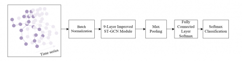
As stated above, accurately identifying and classifying hazardous behaviors in laboratory safety education is very important, as it can prevent accidents and enhance overall safety. Conventional monitoring methods generally rely on manual observations or basic video analysis, however, these methods may not be precise enough and they can’t give real-time feedback. So the application of advanced computer vision and machine learning technologies in monitoring laboratory safety has turned into a particularly important matter. The ST-GCN is a deep learning model specifically designed for processing graph-structured data, and it can give excellent performance in action recognition. The model models the movements of human skeleton in spatio-temporal graphs through graph convolutional networks, so as to effectively capture the relationships between different body parts and the temporal evolution of the movements of students. To enable the hazardous behavior recognition model in laboratory safety education to focus more on identifying specific actions or behavior patterns that may lead to accidents, such as improper handling of chemicals or incorrect instrument operation, this paper improves the model by integrating attention mechanisms and expanding temporal convolution networks into the structure based on ST-GCN. Figure 2 presents the architecture of the hazardous behavior recognition model for laboratory safety education.
Figure 2. Architecture of hazardous behavior recognition model for laboratory safety education
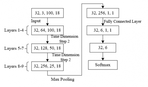
Figure 3. Dimensional changes of model input data
Initially, a spatio-temporal graph is constructed using the spatial configuration of human body joints and their changes over time. In this graph, nodes represent key points of the body, edges represent connections between nodes in space, and the state of the nodes changes over time. In the spatial dimension, the graph convolutional network learns the relationships between each joint and its adjacent nodes. This allows for capturing the interactions between body parts, which is crucial for identifying specific hazardous movement patterns. To capture the temporal evolution of movements, the model extends temporal convolutions. This extension enables the network to better handle long-term dependencies in action sequences and recognize hazardous behaviors that are defined through a series of continuous movements.
Specifically, a single partitioning approach is used to divide the human body into several joints, each potentially corresponding to a body part. The single partitioning method means each joint is divided into an independent part, while adjacent joints represent connections between different body parts. The output of the feature map is usually realized in the form of a matrix, containing features of each joint of the human body. In the $S T-G C N$ framework, these features include the position coordinates of the nodes and possibly other attributes. Figure 3 shows the changes in the dimensions of the model input data. Assuming the output feature map is represented by $d_{O U T}$, the input feature map by $d_{I N}$, the connections between human joints by the adjacency matrix represented by $S$, the self-connection between joints by the identity matrix represented by $U$, and the normalized adjacency matrix by $S^{u u}=\Sigma_k\left(S^{u k}+U^{u k}\right)$, then:
$d_{O U T}=\Lambda_k^{\frac{-1}{2}}(S+U) \Lambda^{\frac{-1}{2}} d_{I N} Q$ (10)
In ST-GCN, the adjacency matrix is used to represent connections between joints. Distance partitioning is usually based on the physical distance between joints, while spatial configuration partitioning depends on the relative position of the joints in space. Decomposing the adjacency matrix reveals the spatial relationships between joints. If the adjacency matrix (S+U) is decomposed into several matrices Sk, then:
$(S+U)=\sum_k S_k$ (11)
Combining the above two formulas yields:
$d_{O U T}=\sum_k \Lambda_k^{\frac{-1}{2}} S_k \Lambda^{\frac{-1}{2}} d_{I N} Q$ (12)
Using the graph convolutional network, the model can learn the spatial features of the joints. This step is achieved by applying convolution operations on the adjacency matrix, capturing the interactions and interconnected relationships between different body parts. The extraction of temporal features is accomplished by analyzing the human skeletal data in consecutive frames. $S T-G C N$ treats the continuous state of joints in a time series as a whole, capturing the development and changes of movements over time through temporal convolutional layers, applying a $\pi \times 1$ convolution operation on $d_{\text {OUT }}$. Assuming the convolution kernel size is represented by $\pi$ and the activation function by $\delta$, the computation formula is:
$d=\delta\left(d_{O U T} * \pi\right)$ (13)
In the context of laboratory safety education, certain joints (such as hands or heads) may be more critical than others, as they are more likely to be involved in hazardous operations. Temporal and spatial attention mechanisms can help the model focus on these critical joints for understanding hazardous behaviors, thereby improving recognition accuracy. Figure 4 shows the architecture of the improved ST-GCN module.
In the field of laboratory safety education, the introduction of a temporal attention mechanism aims to endow the model with the ability to recognize and differentiate the importance of joint movements at different time steps. In the context of laboratory safety education, this means the model needs to identify which sequences of movements might lead to safety risks. Assume the input to the $e$-th spatio-temporal module is represented by $C^{e-1}=\left(c_1, c_2, \ldots, c_{Y e-1}\right) \in E^{B \times V e-1 \times Y e-1}$. The number of channels in the network input data is $V_{e-1}$, the length of the time dimension of the input data is represented by $Y_{e-1}$, the number of frames in the action sequence by $Y_p$, and the activation function by Relu. The spatial matrix is represented by $A \in E^{B \times B}$, and the expression for the spatial attention matrix of joint $C$ at frame $y$ is given by:
$A=C_a \operatorname{Relu}\left(\left(C^{e-1} Q_1\right) Q_2\left(Q_3 C^{e-1}\right)^T+n_a\right)$ (14)
$A_{u, k}^{\prime}=\operatorname{softmax}(A)=\frac{\exp \left(A_{u, k}\right)}{\sum_{k=1}^B \exp \left(A_{u, k}\right)}$ (15)
In the context of laboratory safety education, when using graph convolutional networks to identify and analyze students' actions, further extraction of spatial features of the joints in the network is required. First, construct a graph structure of the joints, then, initialize spatial attention weights and extract node features through graph convolution operations. Graph convolution utilizes the neighborhood information of nodes, aggregating information according to the weight of the nodes. Use one or more spatial attention heads to calculate each node's attention score for its neighboring nodes. After that, normalize the calculated attention scores so that the sum of attention scores for all neighboring nodes of each node equals 1 , and aggregate the features of the neighboring nodes based on each node's attention score to update the current node's feature representation. Assuming the spatial attention matrix is represented by $A^{\prime} \in E^{B \times B}$, and multiplied with $S+U$ and $S_k$ to obtain $(S+U) \otimes A^{\prime}$ and $S_k \otimes A^{\prime}$, thus reasonably allocating the attention of joints in the network. The transformation formula for the output feature map is given by:
$d_{I N}=\Lambda^{\frac{-1}{2}}\left((S+U) \otimes A^{\prime}\right) \Lambda^{\frac{-1}{2}} d_{I N} Q$ (16)
$d_{O U T}=\sum_k \Lambda^{\frac{-1}{2}}\left(S_k \otimes A^{\prime}\right) \Lambda_k^{\frac{-1}{2}} d_{I N} Q$ (17)
The goal of the spatial attention mechanism is to enable the model to better understand and analyze the spatial relationships between joints and the importance of each joint in space. Suppose different frames of the same joint $c_{u k}$ are represented by $Z$, the learning parameters by $C_r, n_r \in E^{Y e-1 Y e-1}$, $W_1 \in E^B, \quad W_2 \in E^{V e-1 \times B}, W_3 \in E^{V e-1}$. The time-related matrix is represented by $R \in E^{Y e-1 Y e-1}$. The degree of interrelation between nodes in different frames is represented by $R_{\mu,k}$, normalized to obtain the time attention matrix represented by $R^{\prime} \in E^{Y e-1 Y e-1}$. The calculation methods for its time-related matrix and time attention matrix are as follows:
$A=C_a \bullet \operatorname{Relu}\left(\left(C^{e-1} W_1\right) W_2\left(W_3 C^{e-1}\right)^Y+n_a\right)$ (18)
$R_{u, k}^{\prime}=\operatorname{softmax}(R)=\frac{\exp \left(R_{u, k}\right)}{\sum_{k=1}^B\left(R_{u, k}\right)}$ (19)
In the context of laboratory safety education, the temporal features of action sequences are crucial, as they can capture the sequence and duration of actions and identify key moments that might lead to accidents. The temporal attention mechanism can identify which time steps are crucial in performing safe operations, for instance, the change in temperature when heating chemicals or the specific moments when mixing reactants. By emphasizing the data of these critical moments, the model can be more focused on recognizing and interpreting actions that might lead to safety issues. Therefore, in this case, the normalized time attention matrix is applied directly to the input data of the current layer. That is, $R^{\prime} \in E^{Y e-1 Y e-1}$ is applied to the input data of the current layer, as follows:
$\begin{aligned} & \hat{Z}^{e-1}=\left(\hat{Z}_1, \hat{Z}_2, \ldots, \hat{Z}_{Y_{e-1}}\right) \\ & =\left(Z_1, Z_2, \ldots, Z_{Y_{e-1}}\right) \otimes R \in E^{B \times V_{e-1} \times Y_{e-1}}\end{aligned}$ (20)
Laboratory safety operations often involve a series of complex movements that unfold over time and contain important sequential information. Additionally, certain actions in safety education may require long preparation and procedural operations. Extended temporal convolution can better understand these dynamic changes and help the model capture these long-term dependencies, rather than just shortterm action sequences. Suppose the residual connection is represented by $D$, the input to the $b$-th layer of temporal convolution by $d^{b-1} I N$, the set of convolutional kernels by $\Gamma$, and the activation function by $\delta$, the transformation formula for the output of the extended temporal convolutional network is given by:
$d_{O U T}^b=d_{I N}^{b-1}+D\left(\Gamma_{* m}, d_{I N}^{b-1}\right)$ (21)
$D\left(\Gamma_{*_m}, d_{I N}^{b-1}\right)=\Gamma_{*_m} * \delta\left(d_{I N}^{b-1}\right)$ (22)
Figure 4. Improved ST-GCN module architecture
Analyzing the data in Table 1, we can observe the impact of different wavelet decomposition levels and threshold rules on the noise reduction of laboratory hazardous behavior data. Signal-to-Noise Ratio (SNR) is an indicator of signal quality, with a higher SNR generally indicating better signal quality. Mean Square Error (MSE) measures the deviation of predicted values from true values, with a lower MSE meaning higher prediction accuracy. The trends in SNR and MSE suggest that as the number of wavelet decomposition levels increases, the noise reduction effect overall improves, proving the effectiveness of wavelet threshold denoising in processing laboratory hazardous behavior data. To choose the most suitable threshold rule and wavelet decomposition level, it is evident that different combinations of rules and levels impact noise reduction differently and should be selected based on specific circumstances. For instance, the Rigrsure rule shows balanced and stable noise reduction performance as levels increase, indicated by improvements in both SNR and MSE. Thus, wavelet threshold denoising is effective in preprocessing laboratory hazardous behavior data. Appropriate selection of threshold rules and decomposition levels can significantly improve data SNR while reducing MSE. However, a balance between enhanced noise reduction performance and computational complexity must be found.
Figure 5 shows the sample sets before and after processing by the adaptive boundary data augmentation algorithm. The upper image (before processing) shows two categories of data: one concentrated on the left side (marked in green), and the other distributed across the right side of the chart. In the upper image, the number of data points on the left is significantly less than those on the right, indicating a clear imbalance in the dataset. In the lower image (after processing), new samples (marked in red) have been added to increase the number of the left-side data category. These new samples are distributed around the original data points, maintaining the original distribution characteristics while increasing the data volume. This treatment increases the number of data points on the left, thus reducing the imbalance between categories. It can be concluded that the adaptive boundary data augmentation algorithm effectively mitigates data imbalance by increasing the number of minority class samples, while maintaining the characteristics of the original data distribution. This method is beneficial for improving machine learning model training, especially in balancing hazardous behavior data in laboratory safety education, contributing to the accuracy of hazardous behavior recognition.
Behaviors 1-8 in Table 2 represent eight hazardous behaviors: not wearing personal protective equipment, incorrect equipment operation, incorrect posture, not closing containers, crowded work spaces, presence of food and beverages, dangerous chemical handling, and lingering in hazardous areas. Analyzing the results in Table 2 for hazardous behavior pattern recognition in different laboratory scenarios, model performance is assessed by observing Recall Rate (R), Precision Rate (P), and F1 Score. For Test Set A, the model shows relatively high recall rates, precision rates, and F1 scores for all behavior patterns, with most indicators above 90%, especially for Behaviors 2, 3, 4, 5, 6, and 7, where F1 scores exceed 97%. For Test Set B, the model exhibits significant variations in recognition performance across different behavior patterns. Particularly, Behaviors 1 and 2 have relatively lower recall and precision rates, with Behavior 1 having the lowest F1 score of 67.45% among all patterns. However, Behavior 3 achieves a 100% recall rate, and Behaviors 5, 7, and 8 have F1 scores over 90%, indicating that the model still maintains high recognition effectiveness in certain behavior patterns. The results from Test Sets A and B suggest that the improved ST-GCN model may exhibit fluctuating recognition performance in different scenarios but overall demonstrates good performance, effectively recognizing hazardous behavior patterns in laboratories. Some behavior patterns show reduced recognition performance in Test Set B compared to Test Set A, possibly due to the complexity of the scene, difficulty of behavior patterns, or coverage of training samples. It can be concluded that the laboratory safety education hazardous behavior recognition method proposed in this paper, based on the improved ST-GCN model, demonstrates good performance in two different test sets, especially excelling in Test Set A. Despite some decrease in recognition of certain behavior patterns in Test Set B, the overall recognition effect remains stable, indicating the model's robustness and generalization capability. Therefore, the model can be considered an effective tool for enhancing the recognition and classification of hazardous behaviors in laboratory safety education.
Table 1. Signal-to-Noise Ratio (SNR) and Mean Square Error (MSE) under different wavelet decomposition levels and threshold rules
|
Threshold Rule |
Wavelet Decomposition Levels (SNR/MSE(×10-2)) |
|||||||||
|
1 |
2 |
3 |
4 |
5 |
6 |
7 |
8 |
9 |
10 |
|
|
Rigrsure |
54.12 |
57.85 |
60.12 |
62.35 |
64.58 |
65.24 |
65.87 |
65.12 |
65.24 |
65.89 |
|
1.42 |
0.68 |
0.38 |
0.22 |
0.16 |
0.13 |
0.13 |
0.13 |
0.13 |
0.13 |
|
|
Heursue |
54.36 |
57.66 |
60.14 |
62.55 |
62.39 |
61.22 |
65.87 |
65..23 |
65.87 |
65.12 |
|
1.31 |
0.68 |
0.37 |
0.22 |
0.16 |
0.14 |
0.13 |
0.13 |
0.13 |
0.13 |
|
|
Sqtwolg |
54.28 |
57.42 |
60.23 |
62.59 |
64.51 |
63.87 |
63.25 |
63.12 |
63.45 |
63.89 |
|
63.2 |
1.29 |
0.67 |
0.37 |
0.22 |
0.17 |
0.17 |
0.21 |
0.23 |
0.28 |
0.28 |
|
Minimacxi |
54.78 |
54.12 |
57.63 |
60.23 |
63.58 |
63.47 |
64.21 |
64.25 |
64.33 |
64.21 |
|
1.31 |
0.69 |
0.37 |
0.21 |
0.15 |
0.14 |
0.14 |
0.18 |
0.21 |
0.21 |
|
Table 2. Performance evaluation of hazardous behavior pattern recognition in different laboratory scenarios
|
Test Set |
Sample Number |
Behavior Pattern |
Recall Rate R |
Precision Rate P |
F1 Score |
|
Test Set A |
2563 |
Behavior 1 |
92.11% |
97.89% |
98.99% |
|
Behavior 2 |
99.04% |
99.04% |
99.06% |
||
|
Behavior 3 |
97.88% |
98.25% |
98.36% |
||
|
Behavior 4 |
97.82% |
97.56% |
97.46% |
||
|
Behavior 5 |
98.78% |
94.10% |
98.73% |
||
|
Behavior 6 |
96.32% |
95.14% |
98.36% |
||
|
Behavior 7 |
98.64% |
97.56% |
97.46% |
||
|
Behavior 8 |
99.12% |
92.32% |
94.67% |
||
|
Test Set B |
2651 |
Behavior 1 |
62.35% |
72.58% |
67.45% |
|
Behavior 2 |
64.23% |
95.36% |
78.23% |
||
|
Behavior 3 |
100% |
73.77% |
84.23% |
||
|
Behavior 4 |
93.68% |
80.69% |
88.99% |
||
|
Behavior 5 |
89.14% |
98.62% |
98.26% |
||
|
Behavior 6 |
91.24% |
92.47% |
91.02% |
||
|
Behavior 7 |
93.44% |
96.37% |
95.77% |
||
|
Behavior 8 |
92.74% |
90.87% |
92.97% |
Figure 5. Sample sets before and after processing by the adaptive boundary data augmentation algorithm
Figure 6. Recall rates for behavior recognition by the model
Figure 7. Precision rates for behavior recognition by the model
From Figure 6, it is observed that the model exhibits high recall rates for all categories of hazardous behaviors, indicating its strong performance in recognizing most of these behaviors. The recall rate for Behavior 3 is as high as 97.6%, for Behavior 2 it is 94.2%, and for Behavior 4, 93.4%. However, some categories, particularly Behaviors 5 and 8, have relatively lower recall rates, at 77.0% and 72.3% respectively. This suggests that the model's effectiveness in recognizing these two types of behaviors is somewhat inferior compared to other categories. Figure 7, also a confusion matrix, focuses on displaying the precision rates (Positive Predictive Value, PPV) and false discovery rates (FDR) for different categories of behavior recognition. In classification problems, precision rate measures how many of the predictions identified as a particular class are correct, while the false discovery rate measures the proportion of incorrect identifications for that class. From Figure 7, it is understood that the values on the diagonal represent the precision rates for each behavior category. For example, the precision rate for Behavior 3 is 95.4%, for Behavior 2 it is 93.9%, and both Behaviors 6 and 7 have precision rates above 90%, at 90.2% and 90.4% respectively. This indicates that the model’s predictions are highly accurate for these categories; when the model identifies a behavior as belonging to these categories, it is likely correct. It can be concluded that the laboratory safety education hazardous behavior recognition model proposed in this paper shows high precision rates in most categories, especially in recognizing Behaviors 3, 2, 6, and 7. However, the precision rates for Behaviors 5, and particularly for Behavior 8, need improvement. Enhancing recognition of these behaviors may involve adjustments to the model structure or further optimization of training data. Overall, the precision rates of this model demonstrate its effectiveness and practicality, especially in the application within the field of laboratory safety education. Nonetheless, optimizing the model to further improve precision rates is crucial for enhancing hazardous behavior recognition.
Figure 8. Accuracy and macro average F1 values of different recognition models
Figure 8 lists the performance evaluation results of five different behavior recognition models—Random Forest (RF), Convolutional Neural Network (CNN), Recurrent Neural Network (RNN), Long Short-Term Memory (LSTM) networks, and the model proposed in this paper, in terms of macro average F1 value and accuracy. The proposed model surpasses the RF, CNN, RNN, and LSTM models in both macro average F1 value and accuracy. It not only shows the best overall accuracy but also achieves a good balance among different categories, which is critically important in practical applications, as it indicates the model's balanced recognition capability across all categories.
Figure 9 demonstrates the model's minimum classification error on different numbers of samples in laboratory safety education hazardous behavior recognition, evaluating the impact of increasing training samples on classification error. With a lower data volume, the model can achieve smaller classification errors, showing its excellent learning capability and adaptability. When the data volume increases to a certain amount, improvement of the model gets gradual, and this may suggest that the model has reached its peak learning ability, or the extra data does not provide enough new information to further enhance the performance of the model. After that, the model shows further performance improvement with a larger data volume, indicating its ability to learn from more data and strengthen its generalization ability. In this way, the proposed model reaches lower minimum classification errors on datasets of various sizes and shows stability and improvement in performance with more data. These results prove that the proposed model’s potential of being used as a useful tool in laboratory safety education, and it can help institutions more accurately identify and prevent potential hazardous behaviors, thereby improving the overall safety levels.
Figure 9. Analysis of model errors
This study centers on using and optimizing machine learning techniques to enhance the recognition of hazardous behaviors in laboratory safety education. In the beginning, this paper discussed the noise problem with the data of laboratory hazardous behaviors and adopted wavelet threshold denoising methods to pre-process the raw data. This method can effectively improve data quality, and had laid a good foundation for subsequent model training and analysis. Then, this paper tackled the data imbalance problem, a common challenge in machine learning, especially in the field of safety education, through the introduction of an adaptive boundary data augmentation algorithm, in this way, the dataset had been balanced, an even representation of each behavior pattern in the model training had been ensured, and the model's ability to recognize minority classes had been enhanced. After that, this paper improved the ST-GCN model to construct spatio-temporal graphs of laboratory hazardous actions, and our innovative approach enables the model to accurately extract spatio-temporal features and achieve efficient hazardous behavior recognition and classification. An evaluation of the comprehensive performance shows that our proposed model outperformed conventional machine learning methods and some existing deep learning models (such as RF, CNN, RNN, and LSTM) in terms of macro average F1 value and accuracy. These results can demonstrate the effectiveness and superiority of the proposed model in fulfilling the task of laboratory hazardous behavior recognition. At last, by analyzing the classification errors attained based on datasets of different sizes, we can see that the proposed model achieved a low error rate with sufficient training samples and showed stability and improvement in its performance as the sample size increased, verifying its good generalizability and practicality.
Findings of this study are of high practical application value in the field of laboratory safety education. Via effective preprocessing of data, discussing the issue of data imbalance, and using the improved ST-GCN model to accurately extract spatio-temporal features, the proposed method shows obvious advantages in recognizing laboratory hazardous behaviors, and it provides a new solution for laboratory safety management, helping to reduce the occurrence of safety accidents and protect the safety of laboratory personnel.
This work was supported by the National Key Research and Development Program of China (Grant No.: 2022YFB4702401), the National Natura Science Foundation of China (Grant No.: 51741502), the Natural Science Foundation of Fuiian Province (Grant No.: 2020J01450), Teaching Reform and Application Practice of Electronic Technology Creation Community (Grant No.: 202102069005), Education Department Project of Fujian Province (Grant No.: JAT211010).
[1] Kim, B.J., Chung, J.B. (2023). Is safety education in the E-learning environment effective? Factors affecting the learning outcomes of online laboratory safety education. Safety Science, 168: 106306. https://doi.org/10.1016/j.ssci.2023.106306
[2] Love, T. S., Roy, K. R., Sirinides, P. (2023). A national study examining safety factors and training associated with STEM education and CTE laboratory accidents in the United States. Safety Science, 160: 106058. https://doi.org/10.1016/j.ssci.2022.106058
[3] Zheng, X., Miao, F., Chakpitak, N., Huang, J., Wang, J. (2021). Discussion of university chemistry laboratory management using DOSA platform and safety education based on blockchain. In Proceedings of the 2021 4th International Conference on Education Technology Management, Tokyo, Japan, pp. 79-85. https://doi.org/10.1145/3510309.3510322
[4] Hassan, N.H.C., Ismail, A.R., Makhtar, N.K., Sulaiman, M.A., Subki, N.S., Hamzah, N.A. (2017). Safety and health practice among laboratory staff in Malaysian education sector. In IOP Conference Series: Materials Science and Engineering, Pahang, Malaysia, pp. 012004. https://doi.org/10.1088/1757-899X/257/1/012004
[5] Micu, L.M., Bordeasu, I., Dionisie, I., Ghiban, B., Gubencu, D. (2023). Influence of aging heat treatment at 1800C on cavitation erosion for aluminum alloy type 5083 in cold rolled state. Journal of Physics: Conference Series, Banja Luka, Bosnia and Herzegovina, pp. 012036. https://doi.org/10.1088/1742-6596/2540/1/012036
[6] Andrei, P., Cazacu, E., Stǎnculescu, M., Andrei, H., Cǎciulǎ, I., Drosu, O. (2023). Thermal behavior of electrical contact for different AC loads. In Proceedings of 2023 10th International Conference on Modern Power Systems (MPS), Cluj-Napoca, Romania, pp. 1-4. https://doi.org/10.1109/MPS58874.2023.10187457
[7] Gao, J., Yi, J., Murphey, Y.L. (2022). Joint learning of video images and physiological signals for lane-changing behavior prediction. Transportmetrica A: Transport Science, 18(3): 1234-1253. https://doi.org/10.1080/23249935.2021.1936279
[8] Su, H., Ying, H., Zhu, G., Zhang, C. (2021). Behavior identification based on improved two-stream convolutional networks and faster RCNN. In Proceedings of the 33rd Chinese Control and Decision Conference (CCDC), Kunming, China, pp. 1771-1776. https://doi.org/10.1109/CCDC52312.2021.9601920
[9] Wang, P., Li, P., Cuntapay, M.C. (2022). Recognition of student emotions in classroom learning based on image processing. Traitement du Signal, 39(4): 1331-1337. https://doi.org/10.18280/ts.390426
[10] Salim, B.W., Hussan, B.K., Ageed, Z.S., Zeebaree, S.R. (2023). Improved transient search optimization with machine learning based behavior recognition on body sensor data. CMC-Computers Materials & Continua, 75(2): 4593-4609. https://doi.org/10.32604/cmc.2023.037514
[11] Zahid, F.B., Ong, Z.C., Khoo, S.Y., Salleh, M.F.M. (2021). Inertial sensor based human behavior recognition in modal testing using machine learning approach. Measurement Science and Technology, 32(11): 115905. https://doi.org/10.1088/1361-6501/ac1612
[12] Wang, S.Y. (2021). Online learning behavior analysis based on image emotion recognition. Traitement du Signal, 38(3): 865-873. https://doi.org/10.18280/ts.380333
[13] He, J., Lin, K.Y., Dai, Y. (2022). A data-driven innovation model of big data digital learning and its empirical study. Information Dynamics and Applications, 1(1): 35-43. https://doi.org/10.56578/ida010105
[14] Chen, H., Jiang, M., Liu, Y., He, J., Li, H. (2020). Review on machine learning and its application in atmospheric science and human behavior recognition. ACM International Conference Proceeding Series, Beijing, China, pp. 98-104. https://doi.org/10.1145/3432291.3432311
[15] Lu, X.H., Yuan, Z.Y., Lin, X.H., Qiu, Z.Q. (2020). Research on behavior recognition method based on machine learning and fisher vector coding. In Multimedia Technology and Enhanced Learning: Second EAI International Conference, ICMTEL 2020, Leicester, UK, pp. 136-147. https://doi.org/10.1007/978-3-030-51100-5_12
[16] Li, X.C., Zhao, J.X., Cong, J.H., Misra, R.D., Wang, X.M., Wang, X.L., Shang, C.J. (2021). Machine learning guided automatic recognition of crystal boundaries in bainitic/martensitic alloy and relationship between boundary types and ductile-to-brittle transition behavior. Journal of Materials Science and Technology, 84: 49-58. https://doi.org/10.1016/j.jmst.2020.12.024
[17] Xie, M., Xiao, Y., Wang, H., Wang, Y. (2021). Recognition and evaluation of driving behavior based on MEMS sensors and machine learning. Advances in Transportation Studies, 55: 185-200.
[18] Zhu, X., Yao, L., Liu, H. (2022). Identification of dangerous sections of highland roads considering different driving behaviors. Journal of Transportation Systems Engineering and Information Technology, 22(6): 172-182. https://doi.org/10.16097/j.cnki.1009-6744.2022.06.018
[19] Xu, Y.X. (2014). Identification of dangerous driving behaviors based on neural network and Bayesian filter. Advanced Materials Research, 846: 1343-1346. https://doi.org/10.4028/www.scientific.net/AMR.846-847.1343
[20] Chu, Y.X., Zhang, J., Yang, L. (2022). Risk identification method of dangerous driving behavior based on sliding window feature fusion. Advances in Transportation Studies, 4: 133-144.
[21] Li, D.H., Sun, J.L., Wu, P., Tao, W., Chen, A. (2022). An identification method of dangerous driving behavior in rush hour based on APRIORI algorithm. Advances in Transportation Studies, 4: 113-122.
[22] Wei, X., Yao, S., Zhao, C., Hu, D., Luo, H., Lu, Y. (2022). Graph convolutional networks (GCN)-based lightweight detection model for dangerous driving behavior. In Wireless Algorithms, Systems, and Applications - 17th International Conference, WASA 2022, Dalian, China, pp. 27-39. https://doi.org/10.1007/978-3-031-19208-1_3
[23] Wei, X., Yao, S., Zhao, C., Hu, D., Luo, H., Lu, Y. (2023). Lightweight multimodal feature graph convolutional network for dangerous driving behavior detection. Journal of Real-Time Image Processing, 20(1): 15. https://doi.org/10.1007/s11554-023-01277-9
[24] Ma, Z., Yang, X., Zhang, H. (2021). Dangerous driving behavior recognition using CA-Center Net. In 2021 IEEE 2nd International Conference on Big Data, Artificial Intelligence and Internet of Things Engineering, ICBAIE 2021, Nanchang, China, pp. 556-559. https://doi.org/10.1109/ICBAIE52039.2021.9390070
[25] Xu, G., Qian, X., Li, X., Wu, W. (2022). Hazard trend identification model based on statistical analysis of abnormal power generation behavior data. International Transactions on Electrical Energy Systems, 2022: 5463109. https://doi.org/10.1155/2022/5463109
[26] Ma, C., Xiao, X., Ma, X. (2017). Identification of dangerous hoisting loads based on vibration characteristics. Journal of Mechanical Engineering Science, 231(21): 4035-4043. https://doi.org/10.1177/0954406216656885