Jayanthi Vajiram*![]() | Sivakumar Shanmugasundaram
| Sivakumar Shanmugasundaram![]()
© 2023 IIETA. This article is published by IIETA and is licensed under the CC BY 4.0 license (http://creativecommons.org/licenses/by/4.0/).
OPEN ACCESS
Pilocytic astrocytoma is a type of tumor related lower-grade glioma (LGG). This brain tumor is more difficult to detect, and treat compared to higher grade gliomas. To understand the complexity of LGGs and related disease of epilepsy and cancer, this study proposes genomic cluster-shape feature selection, feature extraction and segmentation methods. The MRI images provides genomic information of DNA sequencing and gene expression by heat map and feature selected by correlation coefficient of p>0.9. The support vector classifier (SVC) and gaussian kernel (GK) used to quantify the linear relation between two variables, and to measure the similarity between two datapoints with high-dimensional space. The twenty-three relevant features are selected by Random Forest classifier and compared with univariate, recursive feature elimination, and principal component analysis method. The semantic segmentation by UNet has encoder captures context information and decoder enables the precise localisation of the object. The ResNext50 incorporates a cordiality parameter, which used to capture the fine-grained features. The UNet with ResNext50 backbone enhance the performance matrix. The calculated metrics of SVC with GK of selected features (90.05%) were higher than without selected features (63.63%). The feature extraction process by random forest classifier with univariate analysis (85.1%) and recursive feature elimination method (85.71%), and with cross-validation achieving an accuracy of 95.2%. The cross-validation (CV) is used to validate the features, with each combination of k folds being multiplied with different batch sizes and numbers of epochs (80.7%, 90.1%, 92.7%, 96.7%, and 95.6%). The segmentation dice score of UNet (72.13%) and UNet with ResNext50 backbone (89.7%) were used to compare the performance of these features. This study used a dataset of LGG patients and found that their improved segmentation accuracy by up to 9.7% compared to earlier analysis of UNet with other residual network and gives the valuable insight of features associated with tumors and reduce the complexity of treatment.
pilocytic astrocytoma, brain tumor, magnetic resonance imaging, genomic feature selection
Pilocytic astrocytomas occur in 84% of people, who aged between 0-19 years and starts like a benign, low-grade gliomas [1]. These tumors are typically located in the posterior fossa and must be completely resected by effective treatment [2]. The genomic expression and feature selection of MRI images are used for tumor diagnostics and treatment planning [3]. The genomic cluster-shape feature correlation combines the information of both the genomic and imaging modalities of tumor characteristics. The features extracted from the images are used to generate a correlation map. This map can then be used to identify regions of the tumor by selecting the most relevant features, which include DNA mutation, cocluster, mRNA, swarm plot, heatmap. DNA mutation is used to identify mutated genes that may be associated with a disease or phenotype. Cluster of Cluster (CoC) cluster group the genes. mRNA analyze the specific genes. Swarm plot and heatmap are used to visualize the relationship of gene expression. SVC with gaussian kernel is used to classify data points and predict the outcome of a particular gene. Pearson correlation map identify relationships between different gene expressions. The combination of feature selection and SVC with kernel can improve the accuracy and can be used to identify meaningful relationships between genomic and clinical data [4]. Random Forest (RF) is randomly selecting the subset of features, building a decision tree, and then repeating the process for different subsets of features. It works by creating multiple decision trees, also robust to noise and outliers, and can handle both categorical and numerical data. It has been used to classify brain tumors [5]. The backward elimination, forward selection, and random forest can reduce the dimensionality of the dataset found to be correlated with the target class [6]. The recursive feature elimination (RFE) with CV increases the accuracy. The principal component analysis (PCA) reduces the dimensionality of the input data. Tumor detection and classification are explained in this existing article [7, 8].
The UNet architecture consists of convolutional encoder and a symmetric decoder. The encoder connects with ResNext backbone, which consists of a series of convolutions, pooling layers, and non-linear activations. The decoder is made up of up-sampling layers and convolutions to reconstruct the segmented images. The network is trained using a cross-entropy loss and a dice coefficient. It could then be trained on a dataset of images labeled with various types of tumors, to predict the type of tumor present in an image. The UNet with ResNext backbone was used for image segmentation of tumors. It reduces the number of hyperparameters and uses the cardinality function not used by other residual networks. As the network did not start to overfit, no dropout was used. The model overcomes the low contrast, irregular motion, and diverse shapes. This architecture was used to train a limited set of datasets [9].
This work provides the genetic variant analysis. The SVC with a gaussian kernel approach showed improved accuracy when including selected features. Feature extraction using Randon Forest classifier, Univariate and Recursive Feature Elimination methods identified the top selected features of gender, age at initial pathologic, race, and patient id scores. In the Decision Tree method, features were selected based on their ranks ranging from 0 to 3. PCA used to determine the best number of features, which ranged between 2 and 4. Lastly, the segmentation approach provided baseline scores for comparison. The study contributes the understanding of genetic variants present in the analyzed dataset.
Radiomics process extract the quantitative features of prognosis and diagnosis characteristics of brain tumors. A recent study by Sharma et al. [10] of radiomics identify the biomarkers for predicting the survival of patients by clustering algorithm to identify radiomic features that could differentiate between glioblastoma and other brain tumors. They used univariate and multivariate analyses to examine the association between the radiomic features. Studies used a combination of DNA methylation and mRNA expression, and found both were associated with glioblastoma progression and survival rate [10-14]. The identified single nucleotide polymorphisms, linked to specific variations in the human genome using genome-wide association and DNA sequence, used to detect diseases by analyzing the genetic variation [15]. To assess the relevance of features association with the target class using statistical method [16]. The t-test determines correlation coefficient is significantly different from zero, indicating a meaningful association between the features [17]. The meta-feature extractor with hyperparameter tuning extract the new meta-features by using the t-test of the correlation coefficient [18]. Random Forest algorithm exhibited high stability outcomes. The SVM wrapper method and the pearson correlation coefficient gives moderate stability [19]. Li et al. [11] study of glioblastoma progression by support vector machine (SVM) used to identify radiomic features of tumor size, shape, and texture, and were used to distinguish different types of tumors. SVM classifies both linear and non-linear data by mapping it in to a high-dimensional feature space and constructing a hyperplane between different classes of data. Patle and Chouhan [20] study shows the linear, polynomial, gaussian, and radial basis kernel functions are used to map data points in to various feature space. A study by Mazroui et al. [21] and Geng et al. [22], found that random forest classifier with univariate recursive feature elimination with CV, and dimensionality reduction gives accuracy of 92.7% high-grade gliomas [21, 22]. Tang and Liu [23] provides an overview and explanation of cross-validation. The two CV methods are random and individual method [24]. CV mainly used to estimate the properties of bias, variance, and trade-off consistency [25]. CV can be used to identify overfitting, to optimize the selection of features, and to estimate the generalization error, and used to select the best model for a given set of data [26]. Feature selection can be achieved through correlation analysis, detection of mutual information, and statistical tests. The selected features are then used for further subsequent analysis [27]. The other models also are used to segment the brain tumors. The 11-layered deep capsule network used in images of T1, T2 and Flair to detect segmentation scores [28]. AlexNet, VGG16, and ResNet50 models, detect tumor by AUC and ROC scores by with and without data augmentation in Kaggle datasets. Group based classifier use the CNN to classify the brain tumor type. Brain tumor detection by CNN use the loss function of Jensen-Shannon divergence with cross-entropy in small datasets. RescueNet with GAN gives 0.94 dice score and 0.88 Sensitivity in Brat's 2015 dataset [29]. Lightweight CNN used to automatically extract tumor features. The Sarthi study [30] proves the UNet model gives better segmentation results.
UNet has been used to detect and segment brain tumors from MRI scans. This algorithm utilizes a CNN with a symmetric encoder-decoder network architecture. Zhang et al. [31] used a UNet to segment brain tumors from multi-parametric image. Dual path aggregation ResNet50 network (Dpa-R50) network, on the BraTs 2017 dataset achieves a dice similarity coefficient of 0.901 [32, 33]. U-Net based 3D, attention, R2 attention, and modified 3D networks on the Brat's 2020 dataset gives better dice score [34]. The tumor image segmentation based on deep residual networks (ResNets), gives the dice score of 0.93 in Brat's dataset [35].
3.1 Feature selection method
Genomic analysis was then used to extract genetic expressions, intensity, dimension, histogram, and texture features from the identified tumor regions [36]. The brain tumor is caused by the uncontrolled growth of DNA mutations. CoC analysis gives the biologic subtypes of IDH mutation and 1p/19q codeletion status. To stratify tumors, by integrating the analysis of messenger RNA (mRNA), microRNA (miRNA), and DNA methylation (m). Brat's study explains the oncogene amplification maintenance by DNA methylation, mRNA expression, and whole-genome sequencing. The methyl group of DNA is attached to cytosine bases and correlated with the oncogenesis mutations of DNA [37].
Figure 1 explains the proposed image enhancement method. Figure 2 shows the feature selection by genomic analysis and SVC with a gaussian kernel algorithm.
The explanation of the feature selection, extraction, and segmentation techniques along with their mathematical formulations:
a. Feature selection:
Feature selection by correlation analysis, measures the linear relationship between each feature and the target variable. The pearson correlation coefficient (r) is calculated as:
$r=\sum((\times-\bar{X}) *(Y-\bar{Y})) /\left(N * \sigma_X * \sigma_Y\right)$
The two variables are x and y, the means are x̄ and ȳ, the standard deviations are σx and σy, and n is the number of samples. PCC used to rank the selected features, then applying the SVC algorithm with a specific kernel function to evaluate the features.
b. Feature extraction:
b.1. Univariate analyze a single variable through mean, variance, standard deviation, median, mode and range.
$\operatorname{Mean}(\mu)=\left(\mathrm{X}_1+\mathrm{X}_1+\mathrm{X}_1+\cdots+\mathrm{X}_{\mathrm{n}}\right) / \mathrm{n}$
where, X1+X1+X1+…+Xn are the individual observations and n is the total number of observations.
Variance $\left(\sigma^2\right)=\Sigma\left(x_i-\mu\right)^2 / n$
where, xi is an individual observation, μ is the mean, and n is the total number of observations.
$\begin{gathered}\text { Standard Deviation }(\sigma)=\sqrt{\sum\left(\mathrm{x}_{\mathrm{i}}-\mu\right)^2 / \mathrm{n}} \\ \operatorname{Range}=\operatorname{Max}(\mathrm{x})-\operatorname{Min}(\mathrm{x})\end{gathered}$
where, maximum value is Max(x), and minimum value is Min(x) is in the dataset.
b.2. Recursive feature elimination (RFE) is iteratively eliminating less important features from a model
In the original dataset (X20) with p features and the feature selection process as RFE(X20), and the elimination process can be represented recursively as:
$\operatorname{RFE}\left(X^2 0\right)=\operatorname{RFE}\left(X^2 0-\left|F_{-} K\right|\right)$ fork $=1$ to $p$
where, $\operatorname{RFE}\left(\mathrm{X}^2 0-\left|\mathrm{F}_{-} \mathrm{K}\right|\right)$ refers to the recursive feature elimination process on the dataset (X20) after removing the kth feature F_k.
b.3. Decision tree splitting
Decision tree splits the best feature based on intensity and threshold. The metrics used for splitting are Gini index and Information gain:
Gini Index $=1-\sum \pi^2$
Figure 1. The proposed brain tumor MRI image enhancement method
Figure 2. The feature selection by genomic analysis and SVC plus gaussian kernel method
where, pi is the probability of an observation of specific class at the current node.
Information Gain $=$ Entropy $-\Sigma((\mathrm{n} / \mathrm{m}) * \operatorname{Entropy}(\mathrm{m}))$
where, n is the entropy of the parent node, m is the number of observations in the child node after splitting the relevant features.
b.4. Principal Component Analysis (PCA) transform the original variables into a set of linearly uncorrelated variables through eigenvectors and eigenvalues of the covariance matrix of the original data.
Let X be an n x d matrix representing the n data points with d dimensions. The covariance matrix is given by:
$\mathrm{C}=(1 / \mathrm{n}) *-\mathrm{X}^{\mathrm{T}} * \mathrm{X}$
Compute the eigenvectors (v) and eigenvalues (λ) of C. The eigenvectors correspond to the principal components, ranked in descending order based on their eigenvalues.
c. The mathematical formulation for UNet with a ResNext50 backbone involves the use of convolutional neural networks (CNNs) and skip connections. The input image through a ResNext50 backbone, which consists of a series of convolutional layers, batch normalization, and activation functions. This backbone is responsible for extracting higher-level features from the input image. The feature maps extracted by the ResNext50 backbone are then used as input for the UNet architecture.
3.2 The algorithms of support vector classifier (SVC) with gaussian kernel
SVC is a supervised machine learning algorithm that uses the kernel to identify the hyperplane that separates the classes in the dataset. By using the kernel, SVC is able to transform nonlinear data into a higher dimensional space where the data is separable. The kernel allows SVC to manipulate the input data with windows, converting the input into the desired output. The kernel function K(x) is mapped with the dot product of the variables and the mercer theorem, which allows SVC to identify the optimal hyperplane of the dataset.
The standard kernel function is K(x)=1; if f|(x)|<1, and K(x)=0, otherwise:
The dot product of $\mathrm{w}_{\mathrm{k}}^{\mathrm{T}}, \mathrm{w}_{\mathrm{i}}$ is mapped to $\varphi\left(\mathrm{w}_{\mathrm{k}}\right)^{\mathrm{T}}$ and $\varphi\left(\mathrm{w}_{\mathrm{i}}\right)$ As per the mercer theorem, $\mathrm{K}\left(\mathrm{w}_{\mathrm{k}}^{\mathrm{T}}, \mathrm{w}_{\mathrm{i}}\right)=\varphi\left(\mathrm{w}_{\mathrm{k}}\right)^{\mathrm{T}} \varphi\left(\mathrm{w}_{\mathrm{i}}\right)$
The kernel function has gaussian, polynomial and Euclidean distance.
$\left\|\varphi\left(\mathrm{w}_{\mathrm{k}}\right)-\varphi\left(\mathrm{w}_{\mathrm{i}}\right)\right\|^2=\left(\varphi\left(\mathrm{w}_{\mathrm{k}}\right)-\varphi\left(\mathrm{w}_{\mathrm{i}}\right)\right)^{\mathrm{T}}\left(\varphi\left(\mathrm{w}_{\mathrm{k}}\right)-\varphi\left(\mathrm{w}_{\mathrm{i}}\right)\right)$ (1)
$=\mathrm{k}\left(\mathrm{w}_{\mathrm{k}}, \mathrm{w}_{\mathrm{k}}\right)-2 \mathrm{k}\left(\mathrm{w}_{\mathrm{k}} \mathrm{w}_{\mathrm{i}}\right)+\mathrm{k}\left(\mathrm{w}_{\mathrm{i}}, \mathrm{w}_{\mathrm{i}}\right)$ (2)
The feature function similarity has the gaussian kernel function (2):
$\mathrm{K}\left(\mathrm{w}_{\mathrm{k}}^{\mathrm{T}}, \mathrm{w}_{\mathrm{i}}\right)=\exp \left(-\frac{\left\|\left(\mathrm{w}_{\mathrm{k}}\right)^{\mathrm{T}}-\left(\mathrm{w}_{\mathrm{i}}\right)\right\|^2}{2 \sigma^2}\right)$ (3)
The intension is to optimize the weight of each feature of the function g. The Dataset $\mathrm{W} \varepsilon \mathrm{R}^{\mathrm{nwp}}$, which has no of samples (n), no of feature analysis (p), $y_K=\frac{1}{P}, K=1,2,3 \ldots . P$, and the label to be classified as $z_j \in Z$ in which Z=1, 2, …, C. The C is the cluster, so the cluster values vi=[vi1, vi2, ..., vip] was calculated by Eq. (4) i=1, 2, ….., C and J=1, 2, …., n.
$\mathrm{v}_{\mathrm{ik}}=\frac{\sum_{\mathrm{wj}} \in \mathrm{c}_{\mathrm{i}} \mathrm{Vw}_{\mathrm{jk}}}{\left\lceil\mathrm{C}_{\mathrm{i}}\right\rceil}$ (4)
The dissimilarity between the features and the clusters are explained in the Eq. (5).
$\varphi^2\left(\mathrm{w}_{\mathrm{j}}, \mathrm{v}_{\mathrm{i}}\right)=\sum_{\mathrm{k}=1}^{\mathrm{p}}\left\|\varphi\left(\mathrm{w}_{\mathrm{k}}\right)-\varphi\left(\mathrm{w}_{\mathrm{i}}\right)\right\|^2$ and $\varphi^2\left(\mathrm{w}_{\mathrm{j}}, \mathrm{v}_{\mathrm{i}}\right)=\sum_{\mathrm{k}=1}^{\mathrm{p}}\left(\mathrm{K}\left(\mathrm{w}_{\mathrm{k}}, \mathrm{w}_{\mathrm{k}}\right)-2 \mathrm{~K}\left(\mathrm{w}_{\mathrm{k}}, \mathrm{w}_{\mathrm{i}}\right)+\mathrm{K}\left(\mathrm{w}_{\mathrm{i}}, \mathrm{w}_{\mathrm{i}}\right)\right)$ (5)
$\left\|\varphi\left(\mathrm{w}_{\mathrm{k}}\right)-\varphi\left(\mathrm{w}_{\mathrm{i}}\right)\right\|^2=2\left(1-\mathrm{K}\left(\mathrm{w}_{\mathrm{k}}, \mathrm{v}_{\mathrm{i}}\right)\right)=2\left(1-\exp \left(-\frac{\left\|\left(\mathrm{w}_{\mathrm{k}}\right)^{\mathrm{T}}-\left(\mathrm{w}_{\mathrm{i}}\right)\right\|^2}{2 \sigma^2}\right)\right.$ (6)
$\begin{gathered}\min J=\sum_{\mathrm{i}=1}^{\mathrm{c}} \sum_{\mathrm{w}_{\mathrm{j} \in \mathrm{wc}} \mathrm{c}_{\mathrm{j}}} \varphi^2\left(\mathrm{w}_{\mathrm{j}}, \mathrm{v}_{\mathrm{i}}\right)+\delta \sum_{\mathrm{k}=1}^{\mathrm{p}} \mathrm{x}_{\mathrm{k}}{ }^2= \\ \sum_{\mathrm{i}=1}^{\mathrm{c}} \sum_{\mathrm{w}_{\mathrm{j}} \in \mathrm{wc}_{\mathrm{i}}} \mathrm{x}_{\mathrm{k}}\left\|\varphi\left(\mathrm{w}_{\mathrm{jk}}\right)-\varphi\left(\mathrm{v}_{\mathrm{ik}}\right)\right\|^2+\delta \sum_{\mathrm{k}=1}^{\mathrm{p}} \mathrm{x}_{\mathrm{k}}^2, \\ \text { where } \mathrm{x}=\left(\mathrm{x}_1 \ldots \ldots \mathrm{x}_{\mathrm{p}}\right)\end{gathered}$ (7)
$\left(\mathrm{x}_{\mathrm{k}} \in[0,1], \mathrm{k}=1, \ldots, \mathrm{p}\right), \sum_{\mathrm{k}=1}^{\mathrm{p}} \mathrm{x}_{\mathrm{k}}=1$ (8)
$\begin{gathered}\mathrm{w}_{\mathrm{k}}=\frac{1}{\mathrm{p}}+\frac{1}{2 \delta} \sum_{\mathrm{i}=1}^{\mathrm{c}} \sum_{\mathrm{w}_{\mathrm{j}} \in \mathrm{C}_{\mathrm{i}}}\left(\frac{\sum_{\mathrm{k}=1}^{\mathrm{p}}\left\|\varphi\left(\mathrm{w}_{\mathrm{jk}}\right)-\varphi\left(\mathrm{v}_{\mathrm{ik}}\right)\right\|^2}{\mathrm{p}}\right. \left.-\left\|\varphi\left(\mathrm{w}_{\mathrm{jk}}\right)-\varphi\left(\mathrm{v}_{\mathrm{ik}}\right)\right\|^2\right)\end{gathered}$ (9)
$\delta^{\mathrm{t}}=\frac{\alpha \sum_{\mathrm{i}=1}^{\mathrm{C}} \sum_{\mathrm{w}_{\mathrm{j}} \varepsilon \mathrm{wc}} \sum_{\mathrm{k}=1}^{\mathrm{p}} \mathrm{X}_{\mathrm{k}}^{\mathrm{t}-1}\left\|\varphi\left(\mathrm{w}_{\mathrm{jk}}\right)-\varphi\left(\mathrm{v}_{\mathrm{ik}}\right)\right\|^2}{\sum_{\mathrm{k}=1}^{\mathrm{p}}\left(\mathrm{X}_{\mathrm{k}}^{\mathrm{t}-1}\right)^2}$ (10)
Algorithm shows the kernel function of feature selection in the Eq. (10). The input dataset W, label y, $\propto=0.6$ and $\theta=10^{-6}$ and the output gives each gene weight. The initial step starts with count $\mathrm{w}_{\mathrm{k}}^0=\frac{1}{\mathrm{p}}$ to find the weight of each gene (k) by the Eq. (4) and Eq. (5) gives the vi, Eq. (7) gives the J value Eq. (9) gives the weight of gene, Eq. (10) gives the value of δt. The iteration stopping for current iteration(t) and previous iteration (t-1).
$\Delta=\left\|\mathrm{J}^{\mathrm{t}}-\mathrm{J}^{\mathrm{t}-1}\right\|$ if $\Delta>\theta$, then the iteration stops and $\Delta<\theta$, then the iteration goes to the step 2 .
The SVC with the gaussian kernel gives the correlation of p-values with features and the without features. The algorithms create the hyperplane which splits data into two classes. The maximum margin was chosen by the hyperplane. The optimization issue can be defined as the parameter.
C>0 and the $\epsilon_i$ is the slack variables. The slack variables are formulated as =⌈ti-(xi)⌉ if the value is zero for $\epsilon_i$ and classified correctly if $0<\epsilon_i \leq 1$ then xi lies in the margin and classified as correct class, if $\epsilon_i>1$ then the wrong class classified as xi.
$\begin{gathered}\min \frac{1}{2}\|w\|^2+C \sum_{i=1}^N \epsilon_i, \\ \text { so that } y_i\left(w \cdot x_i+b\right) \geq 1-\epsilon_i, i=1,2 \ldots . N, \\ \epsilon_i \geq 0, i=1,2, \ldots N\end{gathered}$ (11)
$\begin{aligned} & \min \frac{1}{2} \sum_{\mathrm{i}=1}^{\mathrm{N}} \sum_{\mathrm{i}=1}^{\mathrm{N}} \alpha_{\mathrm{i}} \alpha_{\mathrm{j}} \gamma_{\mathrm{i}} \gamma_{\mathrm{j}}\left(\mathrm{x}_{\mathrm{i}} \mathrm{x}_{\mathrm{j}}\right)-\sum_{\mathrm{i}=1}^{\mathrm{N}} \alpha_{\mathrm{i}}, \\ & \text { then } \sum_{\mathrm{i}=1}^{\mathrm{N}} \gamma_{\mathrm{i}} \alpha_{\mathrm{i}}=0,0 \leq \propto_{\mathrm{i}} \leq \mathrm{C}, \mathrm{i}=1,2 \ldots . . \mathrm{N}\end{aligned}$ (12)
αi is the Lagrange multiplier. The weight vector is expressed as $\mathrm{w}=\sum_{1=1}^{\mathrm{N}} \alpha_{\mathrm{i}} \gamma_{\mathrm{i}} \mathrm{x}_{\mathrm{i}}$.
The network using the pearson correlation coefficient of p<0.5. To test the accuracy, by two different methods. The selected features give 90% accuracy, and without the selected features gives 71% accuracy. To convert the nonlinear variables into linear equations in high dimensions, the gaussian kernel function was used [38].
Advantages and limitation of different feature selection techniques are wrapper, filter, and embedded methods. The wrapper method optimize the model by multiple times with different feature subsets, that leads to overfit. Filter-based method consider the relevant feature, and not considering their combined features. Embedded feature method supports L1 regularization in linear models.
3.3 Feature extraction methods
Random Forest is an ensemble learning model works by taking a subset of data from the training set and building multiple decision trees on it. It combines the highest accuracy predictions from the decision trees. In order to extract features, it uses a combination of bagging and boosting methods. The recursive feature elimination iteratively removes the features through an early stopping process. PCA reduce the original set of features into a lower dimension of gaussian distribution, by different thresholds and variance. The univariate and multivariate analysis has variance and f-value measures. Univariate analysis with statistical scoring functions determines the best features [39]. Recursive feature elimination (RFE) is used to fit and remove the weakest feature, while Breiman’s method of random forest increases the misclassification rate by randomly permuting features. Guyon’s approach by measuring the loss in the weighted sum of distances from the margin [40]. RFE-CV iteratively removes attributes from the initial set of features, builds on the remaining attributes and calculates the CV score. The process is repeated until the optimum number of attributes is found. The selected attributes give the best score [41].
PCA and LDA are used for dimensionality reduction, but PCA is faster than LDA to compute the eigenvalues and eigenvectors [42, 43].
3.4 Cross validation method
K-fold cross-validation is a resampling method for accurate prediction in machine learning. It involves splitting the data into k portions and k iterations, and use the maximum portion of the data as the test set and the remaining portions as the training set. The k-fold CV method, is often use the training of certain thresholds than the holdout validation approach. Leave-p-out cross-validation (LpoC) is used in small sample size dataset.
In LpoC, the dataset is divided into p parts, each part used as a test set with single iteration and the rest is training set. The performance is evaluated with test set. The process is repeated multiple times and the average performance is taken as a result. This method has limited amount of data and it is not possible to divide it into multiple folds. It can be effectively used for meta-analysis of medical images. It shows the gradient-weighted class activation mapping with diffusion trace images, and gives an accuracy of 0.93% through CV [44-47]. The Figure 3 explains the cross-validation methods.
Figure 3. Fivefold cross validation
3.5 Segmentation models
UNet model classify and to detect small tumor lesions. This method used to identify the specific patterns or features of the tumor and supports for proper diagnosis. UNet is a fully convolutional network (FCN) for fast training with a limited data set [48]. It consists of an encoder, a bottleneck module, and a decoder, which are used to capture context information. The encoder consists of two convolutional layers (33-layers) with ReLu activation, batch normalization, 22 spatial max poolings and drop out. The decoder consists of 22 up-convolutions and a concatenation layer corresponding to the encoder, which is used to deduce the missing spatial information when the segmented feature map is generated by the encoder. The encoder part of the UNet gradually reduces the spatial dimensions of the feature maps while increasing the number of channels. This is typically done through a series of convolutional and pooling layers. Each convolutional layer involves a set of trainable parameters, denoted as W, and a non-linear activation function, such as ReLu. The decoder part of the UNet progressively up samples the feature maps to match the original size of the input image. This is achieved using transposed or up sampling convolutional layers. Skip connections, connects encoder and decoder layers, to preserve spatial information and help with better feature shown in the Figure 4.
ResNext50 is a variant of the ResNet (Residual Network) architecture that has a new dimension called "cardinality". It was designed to alleviate the vanishing gradient problem by using residual connections. It allows the training of significantly deeper networks by incorporating a "grouped convolution" approach. The cardinality of ResNext50 is 64. This means the network contains 64 convolutional layers that are grouped into four stages ResNext50 enhances the learning capabilities and generalization of features as shown in Figure 5.
Figure 4. UNet architecture
Figure 5. ResNext with cardinality-32 architecture
Comparison of UNet with other segmentation models:
The UNet with ResNext50 networks can be used for this task, there are other alternatives are also available. UNet++ is an extension improves the performance by nested and skip connections through fine feature selection. DeepLabv3 network used to capture multi-scale contextual information and progress dilated convolutions to alleviate the gridding effect, which combines atrous spatial pyramid pooling with a modified UNet decoder. Pyramid Scene Parsing Network (PSPNet) utilizes pyramid pooling modules to capture global contextual information at multiple scales to generate more comprehensive segmentations. Fully convolutional network (FCN) is replacing the fully connected layers of traditional CNNs to enable dense pixel-wise predictions. SegNet uses an encoder-decoder structure with skip connections to retain spatial information and refine segmentation results. Each model has its unique performance, and the choice depends on specific requirements of the dataset.
Figure 6. Architecture UNet with ResNext50 backbone
The Figure 6 explains the ResNext50 architecture consists of 32 convolutional blocks (32X4d-setting, 22.2 with residual and 26.1 without residual connections) to increase the cardinality accuracy. The model has 48 convolutional layers and 2 pooling layers and when combined with the UNet model, it provides efficient segmentation through the bottleneck convolutional layer. To improve fast learning, UNet with ResNext50 backbone was used to produce high pixel-wise accuracy. The model downsizes the images into 64×64, 128×128, and 256×256 for faster training and better performance. This combination of UNet with ResNext50 backbone gives high segmentation scores in shorter training times. Best accuracy and epochs coverage are also benchmarked for this model [49].
3.6 Data augmentation
It applies the affine transformations randomly to the image with elastic transform, grid distortion, and optical distortion by Albumentations library. The transformations used are random sized crop, flips, random rotates, transpose, shift scale rotate, brightness contrast, gamma, IAAEmboss, blurr, OneOf,normalize and tensor. It includes various transformations that can be applied to the data to increase its diversity and performance.
3.7 Software used
The recommended approach is executed on a Windows 10 center i7-4710MQ computer chip running at 2.5 GHz (8 central processors). The proposed method is implemented in Python 3.6.5 (matplotlib.pyplot).
The CNN starts the process of the 2D image size of 256×256×3, and outputs 128×128×64 with a 0.1 dropout layer of the same padding, batch normalization, and ReLu activation. The output goes to the next convolutional layer of the same process, resulting in 64×64×64 with a 0.3 dropout layer and an output of 8×8×64. Then, the flattened previous layer results in an output shape of 2556 (tumor-1) and 1373 (normal-0). Finally, a fully connected layer with 128 units as output with high features [50] is used. The fivefold cross-validation of the dataset is separated into one number of five folds (k). The initial process is to split the training (k-1) and testing fold, the process is repeated for each new fold until the accuracy of all folds is returned to balanced classes by randomly splitting the data with the same class ratio throughout the k (5)-fold [51]. The estimator bias increases (k small) and decreases (k high) when evaluated using k-fold cross-validation five times and tested with enlarged images in the dataset by a multiple train-test split process [52]. Hyperparameter tuning was used to analyze the network training method, optimizing the weights and biases before training. Segmentation replaced the fully connected layer with a dense layer to facilitate the tuning process [53], and allowed weight sharing during the training of different images to produce classified images with translation, rotation, and distortion invariance [54]. The ResNext50 backbone consists of a series of convolutional blocks that extract features from the input image. Each block typically includes multiple convolutional layers and residual connections.
In the ResNext backbone UNet has the skip connections are added between the corresponding blocks of the encoder and decoder. The UNet decoder consists of a series of upsampling layers that gradually increase the resolution of the feature maps. Each upsampling layer is typically followed by a convolutional block that further refines the feature representation. The output of the decoder is a segmentation mask that assigns a label to each pixel in the image.
The UNet with a ResNext50 backbone was used to process the dataset. The network was trained using a 1-cycle learning rate and an encoder was used for post-processing. The UNet architecture balanced the multi-scale datasets by performing pixel-wise optimization. The input image size was zero-padded to 512×512 and 2×2 max pooling was performed multiple times. The trained ResNext extracted the features (convolution) and feature maps, halving the channels and performing upsampling (deconvolution). The combination of binary cross entropy and dice loss produced better results. The model was trained with a 1-cycle learning rate for faster response and the dice score was calculated [55]. This architecture allows for accurate and efficient segmentation of LGG regions.
The training process of segmentation model has:
d. Learning Rate: Adam optimization uses a learning rate to control the step size in the parameter space during training. The model weights are updated after each iteration.
e. Loss Function: During training, the model minimize a loss function that quantifies the difference between the predicted segmentation and the ground truth with loss functions of dice and binary cross-entropy.
f. Epochs: The training process involves iteration(epoch) of dataset with multiple times. The number of training epochs determines how many times the model will update its weights based on the training data.
g. Batch Size: The dataset is divided into smaller subsets called batches. The batch size determines how many samples are processed simultaneously before the model updates its weights. Larger batch sizes can increase computational efficiency but may impact model performance.
h. Adam Optimization: Adam is an optimization algorithm that updates the model weights based on the gradients computed from each batch of training data. It overcomes the drawback of stochastic gradient descent by adapting the learning rate for each parameter, offering better convergence and stability for training. The LGG segmentation involves determining the learning rate for optimization, suitable loss function, number of training epochs, appropriate batch size, and utilizing Adam optimization to update the model weights.
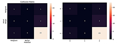
4.1 Evaluation metrics
The confusion matrix was analyzed in terms of true and false positives and negatives. Accuracy was calculated by dividing the total number of correct predictions (true positives + true negatives) by the total number of samples (positives + negatives). The Dice score was used to measure the number of true positives as well as false positives.
$\begin{aligned} & \text { Accuracy }=\frac{(\mathrm{TP}+\mathrm{TN})}{(\mathrm{TP}+\mathrm{FP}+\mathrm{TN}+\mathrm{FN})} \text {, Precision }=\frac{(\mathrm{TP})}{(\mathrm{TP}+\mathrm{FP})} \text {, Recall }=\frac{(\mathrm{TP})}{(\mathrm{TP}+\mathrm{FN})} \text {, } \\ & \mathrm{DSC}=2 \frac{|\mathrm{X} \cap \mathrm{Y}|}{|\mathrm{X}|+|\mathrm{Y}|}=\frac{2 \mathrm{TP}}{2 \mathrm{TP}+\mathrm{FN}+\mathrm{FP}}=2 \frac{\text { Precision } \times \text { Recall }}{\text { Precision }+ \text { Recall }} \text {.}\\ & \end{aligned}$
Adjusting learning rate schedules, regularization techniques, and data augmentation strategies may also impact the number of epochs needed to reach the desired dice score.
Segmentation loss was calculated based on the focal loss. During the model training, the easy negatives overwhelm the loss and gradient to lead by adding more weights.
$\begin{gathered}\text { BCE (Balanced cross Entropy })=\sum_i\left(Y_i \ln \left(P_i\right)+(1-\right. \left.Y_i\right) \ln (1-P)\end{gathered}$
$\left(1-P_i\right)^\gamma$ is the cross-entropy loss, with a tunable focusing parameter with $\gamma \geq 0$.
Focal Loss $P_i=\left(\propto_i\left(1-P_i\right)^\gamma \log P_i\right.$
$P_i=$ unaffected with the small loss
The loss does not affect the number of epochs needed to reach the desired dice score on the training process. Segmentation loss was calculated based on the focal loss. During the model training, the easy negatives overwhelm the loss and gradient to lead by adding more weights.
5.1 Results on feature selection method
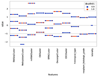
The overall selected features are genetic variants, gentic expression, tumor location, gender, age at initial pathologic, race, and ethnicity, the correlated variable of methylation cluster and CoC cluster, visualization of features, correlation of pair grid plot of miRNA cluster, CN cluster. CoC cluster by swarm plot shows the graph of tumor and non-tumor affected patients by different categorical variables [56]. The correlation coefficient of p>0.9, then the features are eliminated and p<0.9 feature are taken for further analysis. Heat maps visually represent post-processing image gradients, with each pixel having a normalization range of 0 to 1for testing the tumor lesion [57].
Figure 7a and 7b explain the genomic analysis, tumor location, gender, age at initial pathologic, race and ethnicity, and tumor grade evaluate the presence and absence of certain genetic features in each sample. The particular outcome, and can also help to reduce the size of the data set in order to make data analysis more efficient.
(a) (b)
Figure 7. Feature selection based on the genomic analysis, tumor location, gender, age at initial pathologic, race and ethnicity
Figure 8. Correlated variable of methylation and CoC cluster
Figure 9. The features of RPPA and CoC cluster
Figure 10. Correlation of pair grid plot of miRNA cluster and CN cluster-based feature selection
Figure 11. CoC cluster in first swarm plot of tumor and non-tumor affected patient
Figure 8 explains the methylation and CoC clusters are two different types of clusters that are used in bioinformatics and epigenetics research. Methylation clusters are collections of genes that have similar patterns of DNA methylation across one or more cell types or tissues. CoC clusters have similar patterns of co-expression across one or more cell types or tissues. By looking at the correlations between methylation and CoC clusters, gives the insight of molecular mechanisms.
Figure 9 explains the RPPA cluster: The RPPA cluster graph uses a color-coded scale to indicate the expression levels of the proteins. Each protein is represented by a colored square, and the size of the square represents the level of expression.
CoC cluster: The CoC cluster graph uses a color-coded scale to indicate the abundance of the compounds. The abundance of the compound is represented by the size of the coloured square. A larger square indicates higher abundance, while a smaller square indicates lower abundance.
Figure 10 explains the correlation of pair grid plot of miRNA cluster and CN cluster-based, which is used to analyze the relationship between two variables. The plot will show the amount of correlation between the two sets of features, ranging from high correlation (positive or negative). This can help to determine which features are important for a particular task, as well as identify potential relationships between the two sets of features.
Figure 11 explains the CoC cluster in the first swarm plot of tumor and non-tumor affected patients, and identify any potential outliers in the data set. By clustering the points into groups, it can be easier to identify patterns and trends in the data by normal -00 and tumor- 01 patients.
Figure 12 explains the cluster analysis by groups of patients who have similar characteristics, and those who affected by a specific type of tumor.
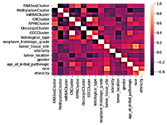
Figure 13 explains the correlation of p>0.9 in a svc with kernel heatmap indicates that the data points are very closely related. This means that the features of the data points are strongly correlated and thus have a high degree of similarity of the data points.
The top selected features from the MRI images are the patient Id,histological type, neoplasm_histologic_grade, tumor_tissue_site, laterality, tumor location, gender, age at initial pathologic, race, and ethnicity, which is used to compare the correlation between features and remove unwanted features. Circulating tumor cell (CTC) clustering can be used to enable metastasis seeding by analyzing the shape of DNA methylation (mi), RNA, and cluster analysis on high dimensional RNA-seq data. To stratify tumors by CoC analysis, compare and correlate features with each other and remove unwanted features.
Figure 12. Cluster of tumor affected patients
Figure 13. Correlation of p>0.9, (SVC +Kernel) heatmap
5.2 Results on feature extraction method
The random forest classifier with univariate, recursive elimination with cross-validation, and principle component analysis are accurate methods for feature extraction and to predict the tumor either malignant or benign. The tree-based method is used to compute the relevance of each feature (0 to 4) based on the feature rank and selects the top-scoring ones based on age, race and gender. The univariate selects the k number of features, and the iterative eliminates the least relevant ones until the desired number of features is reached. The PCA gives the details of number of feature and variance ratio, mean and standard deviation.
Figure 14 explains the univariate and recursive elimination methods are used to extract features from a dataset using series of recursive iterations to identify the important features. The selected features can then be compared to the accuracy of all features in the data set.
Figure 15 shows the recursive elimination with CV to find the most important features with the highest scores. PCA method uses linear algebra to compute the best two selected features based on the highest variance ratio.
Figure 16 explains the construction of decision tree based and on higher rank of the features. RFC provide provides a simple way to identify the most important features in a dataset.
5.3 Results on cross-validation method
The performance of the model is then measured based on the average accuracy of the five-fold CV. It reduces overfitting to improve the performance on unseen data. The bias-variance and tradeoff are used for model fit. The hyperparameter tunning increase the learning rate or regularization strength. It assesses the performance and generalizability of a model, and the importance or relevance of features is calculated based on each iteration to get the average accuracy. The fivefold cross-validation is explained in Figures 17, 18, Table 1 and Table 2.
Figure 14. Feature extraction based on random forest classifier (RFC) with univariate and recursive elimination method
Figure 15. Recursive elimination with cross-validation and PCA method
Table 1. Classification hyperparameters
|
Classification of CNN with Fivefold Cross Validation |
Dropout |
Activation |
Loss |
|
Conv2D (128 to 64(3,3)), Max pooling (2,2) and Dense layer (4) and 64 Neurons |
0.1 |
ReLu/ SoftMax |
Categorical cross Entropy |
|
Conv2D (16 to 8(3,3)), Max pooling (2,2) and Dense layer (4) and 64 Neurons |
0.3 |
ReLu/ SoftMax |
Categorical cross Entropy |
Table 2. Classification scores based on fivefold cross-validation and their metrics
|
Fivefold CV |
Accuracy |
Precision |
Recall |
F1-score |
Normal/Tumor |
Support |
Loss |
|
Prediction 1 |
80.72% |
0.9 |
0.67 |
0.77 |
0 |
131 |
0.39 |
|
0.76 |
0.93 |
0.83 |
1 |
144 |
|||
|
Prediction 2 |
90.18% |
0.9. |
0.87 |
0.88 |
0 |
119 |
0.21 |
|
0.9 |
0.93 |
0.91 |
1 |
156 |
|||
|
Prediction 3 |
92.73% |
0.9 |
0.95 |
0.92 |
0 |
127 |
0.2 |
|
0.96 |
0.91 |
0.93 |
1 |
148 |
|||
|
Prediction 4 |
96.72% |
0.96 |
0.98 |
0.97 |
0 |
142 |
0.11 |
|
0.98 |
0.95 |
0.97 |
1 |
133 |
|||
|
Prediction 5 |
95.63% |
0.93 |
0.99 |
0.96 |
0 |
140 |
0.13 |
|
|
0.98 |
0.93 |
0.95 |
1 |
135 |
Figure 16. Tree-based feature selection (rank) method
5.4 Result on segmentation method
The trained ResNext50 extracted the features (convolution) and feature maps were split into channels, which were then upsampled (deconvolution). The combination of entropy and dice loss gives better results. The network was trained with a learning rate of 1 cycle to improve response time. The segmentation performance was further improved by increasing the number of pixels, which is a promising method for detecting abnormalities in MRI images [58]. The data augmentation was shown in Figure 19. The hyperparameters for the segmentation are discussed in Table 3 and segmentation scores are explained in Table 4.
Table 3. Segmentation hyperparameters
|
Hyperparameters |
UNet |
Uet+ResNext50 |
|
Data split |
Train: (3005, 4) Test: (531, 4), Val: (393, 4) |
Train (3005,4), Test (531,4) Validation (393,4) |
|
Data split based on parameters |
Total 27,003,105 Trainable: 7,945,553 Non-trainable 19,787,002 |
Total (32,561,141), Trainable (9,058,654 Non-trainable (23,502,490) |
|
Losses and Epoch |
0.14823 |
0.19688 and 20 |
|
Dice coefficient |
0.7173 |
0.8951 |
Figure 17. Fivefold cross-validation by performance metrics
Figure 18. Fivefold cross-validation by performance
Figure 19. Data augmentation and visualization
Table 4. Segmentation scores
|
Segmentation Scores |
UNet |
UNet with ResNext50 Backbone |
|
Mean loss on training |
0.377 |
0.133 |
|
Mean DICE on training accuracy |
72.9% |
89.7% |
|
Mean DICE on validation accuracy |
70% |
82% |
|
Batch size |
26 |
26 |
|
Optimizer |
Adam |
Adam |
|
Learning rate |
lr=1e-4 |
lr=5e-5 (20 epochs) |
UNet results the prediction mask, which is compared to the ground truth mask to evaluate the accuracy. The prediction mask highlights the regions in the image that are predicted to belong to the tumor, while the ground truth mask indicates the actual tumor regions as annotated by experts. By comparing these two masks, the performance was calculated. Evaluating segmentation performance involves comparing the generated segmentation maps with the ground truth segmentation, which are explained in Figure 20 and Figure 21.
Segmentation maps that assign a specific label or class to each pixel or region in the input image and highlight the areas of LGG predicted class. Qualitative analysis involves visually inspecting the segmentation maps and comparing them to the ground truth. To consider this by alignment of the predicted boundaries with the actual boundaries, and potential false positives or false negatives. Quantitative metrics can be used to assess the Dice coefficient. It measures the similarity between the predicted and the ground truth segmentation. A high Dice coefficient indicates a strong overlap and agreement between the two predictions. The Dice coefficient of 0.9954 (LGG-BraTs 2018) was achieved by an image-driven UNet model [59].
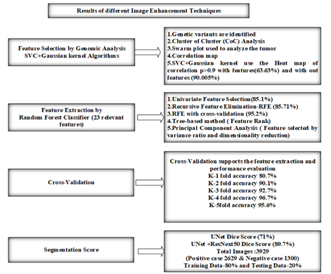
The ground truth performance of the UNet with ResNet50 of earlier results showed an average dice score of 0.80 [60]. The new combination of ResNext50 and UNet can improve the accuracy, in high precision cases. The overall results of this study is shown in the Figure 22.
Figure 20. Prediction mask and Segmentation of Tumor images based on the ResNext50 backbone UNet
Figure 21. Segmentation scores of the UNet and ResNext50
Figure 22. Results of different image enhancement techniques
5.5 Key findings
The key findings are shown in Table 5.
Table 5. Key findings
|
Feature Extraction |
Top Selected Features |
Scores |
|
Genomic analysis |
Genetic variants heatmap correlation
|
p>0.9-Features selected p<0.9-Removed |
|
SVC+gaussian kernel |
With features accuracy With out feature accuracy |
90% 63% |
|
Univariate analysis |
Gender Age at initial pathologic Race Id (Patient) |
0.0955 0.0331 0.3799 1.2768 |
|
Recursive feature elimination |
Id Gender Age at initial pathologic Race |
Accuracy with RF classifier with CV-95.2% |
|
Decision tree feature rank |
Feature 0 Feature 2 Feature 3 Feature 1 |
0.6370 0.2350 0.0713 0.0564 |
|
PCA dimensionality |
Best number of features |
From 2 to 4 |
|
k best values |
Original data K values data |
82,4 82,3 |
Dataset: TCIA-The open access data of https://wiki.cancerimagingarchive.net/display/Public/TCGA-LGG [https://www.kaggle.com/datasets/mateuszbuda/lgg-mri-segmentation]
In addition to the key findings mentioned above, we observed that 80% of LGG patients developed epilepsy during their medication period, while other associated diseases included cancer. Long-term epilepsy associated tumour are low grade, which occur in young patients. This finding of genomic analysis highlights the significant impact of LGG on the development of epilepsy and its association with various forms of cancer. Future directions for this work could include: Incorporating additional feature scale techniques to identify important variables in the genetic variant analysis with different genetic background datasets. Using transform CNN, residual models and segment analysis models in real time datasets to improve the segmentation accuracies are the future scope of this work, and to overcome the limitations of AI models interpretability and potential bias.
[1] Collins, V.P., Jones, D.T.W., Giannini, C. (2015). Pilocytic astrocytoma: Pathology, molecular mechanisms and markers. Acta Neuropathology, 129: 775-788. https://doi.org/10.1007/s00401-015-1410-7
[2] Knight, J., De Jesus, O. (2023). Pilocytic Astrocytoma Treasure Island (FL). StatPearls Publishing.
[3] Abusamra, H. (2013). A comparative study of feature selection and classification methods for gene expression data of glioma. Procedia Computer Science, 23: 5-14. https://doi.org/10.1016/j.procs.2013.10.003
[4] Tran, K.M., Chandra, A. (2019). Feature selection based on genomic analysis of DNA mutation, cocluster, mRNA, swarm plot, heatmap and SVM with kernel. BMC Bioinformatics, 20(1): 522.
[5] Arora, V., Agarwal, S., Rani, S. (2021). Brain tumor classification using decision tree and random forest. IEEE Access, 9: 468-476. https://doi.org/10.1109/access.2020.3035976
[6] Khan, M.M., Ahmad, F., Khan, M.M. (2021). Feature selection using Pearson correlation coefficient and corelation map. International Journal of Bioinformatics Research and Applications, 17(2): 150-159.
[7] Amin, J., Sharif, M., Haldorai, A. (2022). Brain tumor detection and classification using machine learning: A comprehensive survey. Complex & Intelligent Systems, 8: 3161-3183. https://doi.org/10.1007/s40747-021-00563-y
[8] Zhang, W., Wu, Y., Yang, B., Hu, S., Wu, L., Dhelim, S. (2021). Overview of multi-modal brain tumor MR image segmentation. Healthcare, 9: 1051. https://doi.org/10.3390/healthcare9081051
[9] Xie, X., Li, L., Lian, S., Chen, S., Luo, Z. (2020). SERU: A cascaded SE-ResNeXT U-Net for kidney and tumor segmentation. Concurrency and Computation: Practice and Experience, 32(14): e5738. https://doi.org/10.1002/cpe.5738
[10] Sharma, M., Sharma, R., Prakash, S., Sharma, A. (2020). Brain tumor segmentation using deep learning: A comprehensive review. Frontiers in Bioengineering and Biotechnology, 8: 597. https://doi.org/10.3389/fbioe.2020.00597
[11] Li, H., Zhang, J., Chen, X., (2020). Brain tumor segmentation using deep learning and radiomics. Medical Image Analysis, 62: 101685. https://doi.org/10.1016/j.media.2020.101685
[12] Zhao, Y., Li, Y. (2019). Brain tumor segmentation using deep learning with a combination of DNA methylation and mRNA expression data. BMC Bioinformatics, 20(1): 568. https://doi.org/10.1186/s12859-019-3028-9
[13] Park, D., Kim, H., Kim, Y., Park, J. (2021). Brain tumor segmentation using deep learning and DNA methylation. BMC Medical Imaging, 21(1): 1-13. https://doi.org/10.1186/s12880-021-00502-2
[14] Zhang, Y., Li, R., Wang, Y. (2021). Brain tumor segmentation using deep learning: A review. Computers in Biology and Medicine, 132: 103750. https://doi.org/10.1016/j.compbiomed.2020.103750
[15] Pudjihartono, N., Fadason, T., Kempa-Liehr, A.W., O’Sullivan, J.M. (2022). A review of feature selection methods for machine learning-based disease risk prediction. Front Bioinform, 2: 927312. https://doi.org/10.3389/fbinf.2022.927312
[16] Danasingh, A.A., Subramanian, A., Epiphany, J.L. (2020). Identifying redundant features using unsupervised learning for high-dimensional data. SN Applied Sciences, 2: 1367. https://doi.org/10.1007/s42452-020-3157-6
[17] Blessie, E.C., Karthikeyan, E. (2012). Sigmis: A feature selection algorithm using correlation based method. Journal of Algorithms & Computational Technology, 6(3): 385-394. https://doi.org/10.1260/1748-3018.6.3.385
[18] Alcobaça, E., Siqueira, F., Rivolli, A., Garcia, L.P., Oliva, J.T., De Carvalho, A.C. (2020). MFE: Towards reproducible meta-feature extraction. The Journal of Machine Learning Research, 21(1): 4503-4507. https://doi.org/10.5555/3455716.3455827
[19] Cueto-López, N., García-Ordás, M.T., Dávila-Batista, V., Moreno, V., Aragonés, N., Alaiz-Rodríguez, R. (2019). A comparative study on feature selection for a risk prediction model for colorectal cancer. Computer Methods and Programs in Biomedicine, 177: 219-229. https://doi.org/10.1016/j.cmpb.2019.06
[20] Patle, Chouhan, D.S. (2013). SVM kernel functions for classification. International Conference on Advances in Technology and Engineering (ICATE), 1-9, https://doi.org/10.1109/ICAdTE.2013.6524743
[21] Mazroui, B., Youssef, M., Kessentini, M. (2018). An empirical evaluation of software engineering challenges and best practices associated with agile scrum. Journal of Systems and Software, 142: 131-151. https://doi.org/10.1016/j.jss.2018.05.036
[22] Geng, X., Wang, Q., Li, Y. (2018). A decision tree-based algorithm for multi-objective optimization. In 2018 IEEE International Conference on Systems, Man, and Cybernetics, pp. 2731-2736.
[23] Tang, L., Liu, H. (2009). Cross-validation. In: LIU, L., ÖZSU, M.T. (eds) Encyclopedia of Database Systems. Springer, Boston, MA. https://doi.org/10.1007/978-0-387-39940-9_565
[24] Ferdinandy, B., Gerencsér, L., Corrieri, L., Perez, P., Újváry, D., Csizmadia, G., Miklósi, Á. (2020). Challenges of machine learning model validation using correlated behaviour data: Evaluation of cross-validation strategies and accuracy measures. PloS One, 15(7): e0236092. https://doi.org/10.1371/journal.pone.0236092
[25] Yates, L.A., Aandahl, Z., Richards, S.A., Brook, B.W. (2023). Cross validation for model selection: A review with examples from ecology. Ecological Monographs, 93(1): e1557. https://doi.org/10.1002/ecm.1557
[26] Khan, A.A. (2020). Application of machine learning and cross-validation techniques for the analysis of brain tumor datasets. Computational and Structural Biotechnology Journal, 18(6): 1535-1544. https://doi.org/10.1016/j.csbj.2020.05.001
[27] Moscovich, A., Rosset, S. (2022). On the cross-validation bias due to unsupervised preprocessing. Journal of the Royal Statistical Society Series B: Statistical Methodology, 84(4): 1474-1502. https://doi.org/10.1111/rssb.12537
[28] Sille, R., Choudhury, T., Chauhan, P., Sharma, D. (2021). A systematic approach for deep learning-based brain tumor segmentation. Ingénierie des Systèmes d’Information, 26(3): 245-254. https://doi.org/10.18280/isi.260301
[29] Aggarwal, M., Tiwari, A.K., Sarathi, M.P. (2022). Comparative analysis of deep learning models on brain tumor segmentation datasets: BraTS 2015-2020 datasets. Revue d'Intelligence Artificielle, 36(6): 863-871. https://doi.org/10.18280/ria.360606
[30] Sarthi, G., Chikkaguddaiah, N. (2023). Human brain tumor detection and segmentation for MR image. Revue d'Intelligence Artificielle, 37(1): 147-153. https://doi.org/10.18280/ria.370118
[31] Zhang, Q., Wang, Y., Zhang, Y., Zhao, R., Li, T. (2021). Multi-parametric MRI brain tumor segmentation with a dual-U-net model. Computers in Biology and Medicine, 124: 103936.
[32] Naeem, M.A., Rehman, M.A.U., Ullah, R., Kim, B.S. (2020). A comparative performance analysis of popularity-based caching strategies in named data networking. IEEE Access, 8: 50057-50077. https://doi.org/10.1109/ACCESS.2020.2980385
[33] Naeem, M.A., Rehman, M.A.U., Ullah, R., Kim, B.S. (2020). A comparative performance analysis of popularity-based caching strategies in named data networking. IEEE Access, 8: 50057-50077. https://doi.org/10.1109/ACCESS.2020.2980385
[34] Banerjee, S., Ghosh, S., Sinha, S. (2020). Brain tumor segmentation using Dual Path Aggregation ResNeXt50 Network. In 2020 International Conference on Computing, Communication and Automation, pp. 1-5.
[35] Yousef, R., Khan, S., Gupta, G., Siddiqui, T., Haq, M.A. (2023). U-Net-based models towards optimal MR brain image segmentation. Diagnostics, 13(9): 1624. https://doi.org/10.3390/diagnostics13091624
[36] Shehab, L.H., Fahmy, O.M., Gasser, S.M., El-Mahallawy, M.S. (2021). An efficient brain tumor image segmentation based on deep residual networks (ResNets). Journal of King Saud University-Engineering Sciences, 33(6): 404-412. https://doi.org/10.1016/j.jksues.2020.06.001
[37] Nakamoto, T., Takahashi, W., Haga, A., Takahashi, S., Kiryu, S., Nawa, K., Nakagawa, K. (2019). Prediction of malignant glioma grades using contrast-enhanced T1-weighted and T2-weighted magnetic resonance images based on a radiomic analysis. Scientific Reports, 9(1): 1-12. https://doi.org/10.1038/s41598-019-55922-0
[38] Cancer Genome Atlas Research Network. (2015). Comprehensive, integrative genomic analysis of diffuse lower-grade gliomas. New England Journal of Medicine, 372(26): 2481-2498. https://doi.org/10.1056/NEJMoa1402121
[39] Rustam, Z., Kharis, S.A.A. (2020). Comparison of support vector machine recursive feature elimination and kernel function as feature selection using support vector machine for lung cancer classification. In Journal of Physics: Conference Series, 1442(1): 012027. https://doi.org/10.1088/1742-6596/1442/1/012027
[40] Le, N.Q.K., Kha, Q.H., Nguyen, V.H., Chen, Y.C., Cheng, S.J., Chen, C.Y. (2021). Machine learning-based radiomics signatures for EGFR and KRAS mutations prediction in non-small-cell lung cancer. International Journal of Molecular Sciences, 22(17): 9254. https://doi.org/10.3390/ijms22179254
[41] Escanilla, N.S., Hellerstein, L., Kleiman, R., Kuang, Z., Shull, J., Page, D. (2018). Recursive feature elimination by sensitivity testing. In 2018 17th IEEE International Conference on Machine Learning and Applications (ICMLA), Orlando, FL, USA, pp. 40-47. https://doi.org/10.1109/ICMLA.2018.00014
[42] Mustaqim, A.Z., Adi, S., Pristyanto, Y., Astuti, Y. (2021). The effect of recursive feature elimination with cross-validation (RFECV) feature selection algorithm toward classifier performance on credit card fraud detection. In 2021 International Conference on Artificial Intelligence and Computer Science Technology (ICAICST), Yogyakarta, Indonesia, pp. 270-275. https://doi.org/10.1109/ICAICST53116.2021.9497842
[43] Guo, W., Zhou, Z.Z. (2022). A comparative study of combining tree-based feature selection methods and classifiers in personal loan default prediction. Journal of Forecasting, 41(6): 1248-1313. https://doi.org/10.1002/for.2856
[44] Hidayat, E., Fajrian, N.A., Muda, A.K., Huoy, C.Y., Ahmad, S. (2011). A comparative study of feature extraction using PCA and LDA for face recognition. In 2011 7th International Conference on Information Assurance and Security (IAS), Melacca, Malaysia, pp. 354-359. https://doi.org/10.1109/ISIAS.2011.6122779
[45] Yadav, S., Shukla, S. (2016). Analysis of k-fold cross-validation over hold-out validation on colossal datasets for quality classification. In 2016 IEEE 6th International Conference on Advanced Computing (IACC), Bhimavaram, India, pp. 78-83. https://doi.org/10.1109/IACC.2016.25
[46] Malhotra, R., Meena, S. (2021). Empirical validation of cross-version and 10-fold cross-validation for defect prediction. In 2021 Second International Conference on Electronics and Sustainable Communication Systems (ICESC), Coimbatore, India, pp. 431-438. https://doi.org/10.1109/ICESC51422.2021.9533030
[47] Jiang, X., Wang, Q., Du, M., Ding, Y., Hao, J., Li, Y., Liu, Q. (2022). Research on GIS isolating switch mechanical fault diagnosis based on cross-validation parameter optimization support vector machine. In 2022 IEEE International Conference on High Voltage Engineering and Applications (ICHVE), Chongqing, China, pp. 1-4. https://doi.org/10.1109/ICHVE53725.2022.9961557
[48] Artzi, M., Redmard, E., Tzemach, O., Zeltser, J., Gropper, O., Roth, J., Ben-Sira, L. (2021). Classification of pediatric posterior fossa tumors using convolutional neural network and tabular data. IEEE Access, 9: 91966-91973. https://doi.org/10.1109/ACCESS.2021.3085771
[49] Yin, Q., Li, Y.F., Li, J.J., Zheng, X., Guo, P. (2023). Pulsar-candidate selection using a generative adversarial network and ResNeXt. The Astrophysical Journal Supplement Series, 264(1): 2. https://doi.org/10.3847/1538-4365/ac9e54
[50] Tiwari, P., Pant, B., Elarabawy, M.M., Abd-Elnaby, M., Mohd, N., Dhiman, G., Sharma, S. (2022). CNN based multiclass brain tumor detection using medical imaging. Computational Intelligence and Neuroscience, 2022: 1830010. https://doi.org/10.1155/2022/1830010
[51] Taher, F., Shoaib, M.R., Emara, H.M., Abdelwahab, K.M., El-Samie, A., Fathi, E., Haweel, M.T. (2022). Efficient framework for brain tumor detection using different deep learning techniques. Frontiers in Public Health, 10: 959667. https://doi.org/10.3389/fpubh.2022.959667
[52] Hilles, S.M., Saleh, N.S. (2021). Image segmentation and classification using CNN model to detect brain tumors. In 2021 2nd International Informatics and Software Engineering Conference (IISEC), Ankara, Turkey, pp. 1-7. https://doi.org/10.1109/IISEC54230.2021.9672428
[53] Khan, M.S.I., Rahman, A., Debnath, T., Karim, M.R., Nasir, M.K., Band, S.S., Dehzangi, I. (2022). Accurate brain tumor detection using deep convolutional neural network. Computational and Structural Biotechnology Journal, 20: 4733-4745. https://doi.org/10.1016/j.csbj.2022.08.039
[54] Li, J., Wang, P., Li, Y., Zhou, Y., Liu, X., Luan, K. (2018). Transfer learning of pre-trained Inception-v3 model for colorectal cancer lymph node metastasis classification. In 2018 IEEE International Conference on Mechatronics and Automation (ICMA), Changchun, China, pp. 1650-1654. https://doi.org/10.1109/ICMA.2018.8484405
[55] Xu, Y., He, X., Xu, G., Qi, G., Yu, K., Yin, L., Chen, H. (2022). A medical image segmentation method based on multi-dimensional statistical features. Frontiers in Neuroscience, 16: 1009581. https://doi.org/10.3389/fnins.2022.1009581
[56] Lim, A.H., Chan, J.Y., Yu, M.C., Wu, T.H., Hong, J.H., Ng, C.C.Y., Hsieh, S.Y. (2022). Rare occurrence of aristolochic acid mutational signatures in oro-gastrointestinal tract cancers. Cancers, 14(3): 576. https://doi.org/10.3390/cancers14030576
[57] Esmaeili, M., Vettukattil, R., Banitalebi, H., Krogh, N.R., Geitung, J.T. (2021). Explainable artificial intelligence for human-machine interaction in brain tumor localization. Journal of Personalized Medicine, 11(11): 1213. https://doi.org/10.3390/jpm11111213
[58] Vu, M.H., Grimbergen, G., Nyholm, T., Löfstedt, T. (2020). Evaluation of multislice inputs to convolutional neural networks for medical image segmentation. Medical Physics, 47(12): 6216-6231. https://doi.org/10.1002/mp.14391
[59] Arora, A., Jayal, A., Gupta, M., Mittal, P., Satapathy, S.C. (2021). Brain tumor segmentation of MRI images using processed image driven U-Net Architecture. Computers, 10: 139. https://doi.org/10.3390/computers10110139
[60] Aboussaleh, I., Riffi, J., Fazazy, K.E., Mahraz, M.A., Tairi, H. (2023). Efficient U-Net architecture with multiple encoders and attention mechanism decoders for brain tumor segmentation. Diagnostics, 13(5): 872. https://doi.org/10.3390/diagnostics13050872