Doma Murali Krishna*![]() | Sanjay Kumar Sahu
| Sanjay Kumar Sahu![]() | Grlvnsrinivasa Raju
| Grlvnsrinivasa Raju![]()
© 2023 IIETA. This article is published by IIETA and is licensed under the CC BY 4.0 license (http://creativecommons.org/licenses/by/4.0/).
OPEN ACCESS
The global rise of skin cancer, accredited primarily to abnormal radiation-induced cellular growth, has resulted in millions of fatalities. Early detection and accurate diagnosis can potentially ameliorate the survival rate. However, traditional methods for skin lesion detection and classification (SLDC) employing machine learning (ML) and deep learning (DL) models have demonstrated limitations, notably higher stochastic gradient issues, increased mispredictions, elevated training losses, and decreased detection and classification accuracy. Addressing these limitations, we present an optimized Hybrid SLDC network (HOS-Net). The initial phase of the study saw the augmentation of the ISIC-2019 dataset, thereby increasing the quantity of images. These images were then preprocessed to normalize their size and data type. A Deep Convolutional Inverse Graphics Network (DCIGN) was subsequently developed to identify disease-affected regions from the preprocessed images. Following this, a Hybrid Deep Kohonen Network (HDKN) was introduced to extract disease-specific and disease-dependent features from the segmented images. Additionally, a Swarm-based Pelican Optimization Algorithm (SPOA) was implemented to extract the optimal features from the HDKN output features. Ultimately, a Deep Echo Network Machine (DENM) was utilized to classify various disease types using the pre-trained SPOA features. Simulations conducted on the ISIC-2019 dataset revealed that the proposed HOS-Net model achieved superior performance, with an accuracy of 99.13%, precision of 99.13%, recall of 99.25%, and an F1-score of 99.56%. This performance signifies the model's capability to accurately classify and capture positive cases in the data.
skin cancer classification, deep convolutional inverse graphics network, skin lesion detection, swarm-based pelican optimization, hybrid deep Kohonen network, deep echo network machine
Skin cancer is a burgeoning health issue of global significance, with an array of contributing factors such as tobacco use, shifting climatic conditions, alcohol consumption, dietary habits, viral infections, radiation exposure, and lifestyle choices driving the escalating rate of diagnoses [1]. As one of the most lethal forms of cancer, skin cancer is also notably prevalent, often manifesting as aberrant growth of skin cells. The incidence of skin cancer is rising, with an alarming 5.4 million new cases diagnosed annually in the United States alone [2]. The World Health Organization (WHO) has reported an astonishing 53% annual increase in the incidence of melanoma cases, with a projected upswing in the mortality rate in the forthcoming years. Early detection is paramount, as it dramatically enhances survival rates, with the chances of survival skyrocketing to nearly 97% when skin cancer is detected early, as opposed to a mere 14% when diagnosed at an advanced stage.
The most widespread types of non-melanocytic skin cancer are basal cell carcinoma (BCC) and squamous cell carcinoma (SCC). These types, BCC and SCC, are more prevalent than melanoma, with yearly incidence estimates of 4.3 million and 1 million cases, respectively. However, these figures may be underestimations [3]. Prompt diagnosis is crucial in boosting survival probabilities, as the disease's deeper penetration into the skin drastically diminishes survival rates. Currently, medical practitioners employ polarized light magnification and dermoscopy for visual examination, taking into account factors such as patient's ethnicity, sun exposure, social habits, and medical history to facilitate diagnosis [4]. Nevertheless, the process of analyzing biopsied lesions remains labor-intensive and time-consuming, impeding timely medical interventions for skin cancer detection.
Motivation: Despite advancements, the accuracy of skin cancer diagnosis remains heavily dependent on the expertise of seasoned dermatologists, with a recommended accuracy rate exceeding 80%. Given the global dearth of proficient dermatologists, the development of image analysis algorithms becomes crucial for early-stage skin cancer diagnosis and to address the challenges presented by the specialist shortage.
In recent years, artificial intelligence (AI)-enabled computer-aided diagnostics (CAD) technologies [5] have emerged as a potent tool in the realm of medical imaging. AI-based algorithms have demonstrated superior performance compared to physicians in diagnosing various diseases [6]. AI has found applications in the detection of a diverse set of afflictions, such as brain tumors, breast cancer, esophageal cancer, lung cancer, and skin lesions. Dermoscopy, CT scans, and MRIs have been instrumental in skin imaging, paving the way for the development of automated CAD systems [7]. The proliferation of skin lesion images and expert-provided annotations has spurred research in this field, especially in the era of high-speed internet, powerful computing machines, and reliable cloud storage, enabling conventional computers to function as advanced medical devices.
Problem Statement: A significant hurdle in AI-driven skin cancer diagnosis is the management of imbalanced datasets, where certain classes may be overrepresented due to a limited number of examples. Data augmentation, the process of modifying existing training data to generate new samples, has shown promise in ameliorating this issue, particularly in medical diagnostic imaging. By utilizing data augmentation techniques, AI models can better manage unbalanced datasets and enhance classification accuracy. Numerous traditional machine learning algorithms heavily depend on handcrafted feature engineering. Extracting pertinent features from raw data can be laborious and time-intensive, and the performance of these models is largely contingent on the quality of the selected features. Classic machine learning models are prone to overfitting (adhering excessively to the training data) or underfitting (oversimplifying the data). Striking a balance between bias and variance is pivotal, necessitating expertise and meticulous tuning. Fine-tuning hyperparameters in conventional AI models can be a time-intensive process requiring expert knowledge, rendering the optimization process challenging and less accessible for non-experts.
In this study, we aim to augment the evolution of AI-driven skin cancer diagnosis by proposing a novel approach that addresses the limitations of traditional methodologies. Our research concentrates on enhancing diagnostic accuracy, particularly in early-stage detection, and tackling the issues associated with imbalanced datasets. By bolstering the capabilities of AI-based diagnostic systems, we strive to boost early diagnosis rates and, ultimately, contribute to improving skin cancer survival rates.
Key Contributions: The unique contributions of this work are as follows:
The remainder of the paper is organized as follows: Section 2 presents a literature survey of both segmentation and classification approaches. Section 3 provides a comprehensive explanation of the HOS-Net's operation, detailing its various algorithms. Section 4 presents the simulation results of the HOS-Net and compares them with conventional AI, ML, and DL methods. Finally, Section 5 concludes the paper, discussing future prospects.
This section covers the methods developed by authors in the field of skin cancer segmentation, and classification. Further, the survey also contains the cumulative problems of each method. These methods encompass a wide range of approaches, from traditional image processing techniques to state-of-the-art deep learning algorithms. The survey aims to explore and analyze the existing body of research on skin lesion segmentation and classification methods. Different techniques are analysed with strengths, limitations, and performance in handling diverse skin lesion images. The survey helped to identify common trends, advancements, and gaps. The survey also provided insights into potential areas for further research and development of more robust and reliable CAD systems for skin lesion diagnosis.
2.1 Survey on SLDC segmentation methods
The authors [8] used a melanoma segmentation method based on U-net and DL networks. IMLT-DL based skin lesion segmentation and classification model was implemented in the research [9] along with MFO. In the research [10], the authors developed three DL based models UNET, RESUNET, improved RESUNET for skin lesion segmentation. Table 1 analyses the key findings, advantages, and limitations of various SLDC segmentation methods. Using a deep-learning based methodology, especially a multi-layer residual convolutional neural network (MLR-CNN), and fuzzy k-means clustering, the authors of the research [11] provided a completely automated method for segmenting cutaneous melanoma at its early stage (FKM). Later-stage cutaneous melanoma was also categorized by the study's authors [12]. Using many clinical images, the supplied method is tested to determine whether it may aid the dermatologist in making a prompt diagnosis of this potentially lethal disorder. Using support vector machines, random forests, deep neural networks, neural networks, and K-nearest neighbor networks, the authors of the research [13] demonstrated how these methods was used to differentiate between malignant and benign skin tumors. The authors of the research [14] presented a two-stream deep neural network data fusion framework for classifying a wide variety of skin cancers. The proposed strategy integrates two distinct methods: A first proposal is made for improving contrast via fusion. When the images have been enhanced, they are fed into a pretrained DenseNet201 architecture. Following that, the recovered features are optimized using a method called skewness-controlled moth-flame optimization (MFO). Using swarm intelligence (SI) algorithms, the authors of the research [15] explain how to separate the region of interest (RoI) around skin lesions in dermoscopy images. The Grasshopper Optimization Algorithm achieves the best RoI extraction results (GOA). In the research [16], the authors demonstrated their efforts in dermoscopy image segmentation. To fine-tune the network's hyper-parameters, a novel method called Exponential Neighborhood Grey Wolf Optimization (EN-GWO) is used. The authors of the research [17] created a stacked ensemble architecture based on explainable CNNs with the goal of early detection of melanoma skin cancer. The notion of transfer learning is used inside the stacking ensemble framework, which involves the assembly of numerous CNN sub-models that each carry out the same classification job. In the research [18], the authors proposed InSiNet, a convolutional neural network that uses deep learning to distinguish between benign and malignant lesions. The mapped images and newly acquired features are subjected to transfer learning before a deep learning model known as ResNet-50 [19] is used to analyse them. When the retrieved features have been further optimised using an enhanced grasshopper optimization technique, they are then categorised with a naive Bayes classifier. The authors of the research [20] established a hierarchical framework for the segmentation of skin lesions using a three-step superpixel lesion segmentation process. In the article [21], the authors described DL as a technique for precisely removing a lesion zone from a sample. To begin, the image is segmented using Enhanced Super-Resolution Generative Adversarial Networks (ESRGAN), which is a technique that is used to increase the image's overall quality. The authors of the research [22] described a segmentation approach that was used to retrieve the afflicted region from an image of skin cancer. Because of this, the images are used as input for Fuzzy U-net, which does segmentation, and May Fly Optimizer, which aims to enhance the range of accuracy, is used to optimise the results. SCDNet is the term given to the model that was published by the authors in the research [23]. This model combines Vgg16 for the purpose of segmentation with CNN to classify the various forms of skin cancer. Using a collection of images, the authors of the research [24] proposed an optimization-based algorithm that could detect skin cancer. The segmentation is taken out utilising the U-RP-Net that was suggested. The Aquila Whale Optimization (AWO) method is used to integrate the U-Net and RP-Net models, which then results in the suggested U-RP-Net model being produced.
Table 1. Summary of SLDC segmentation approaches
|
Ref. No. |
Key Findings |
Advantages |
Limitations |
|
[11] |
Automated segmentation of early-stage melanoma |
Deep learning-based methodology |
Lack of comparison with other methods |
|
[12] |
Categorization of later-stage melanoma |
Fuzzy k-means clustering |
Limited validation on diverse datasets |
|
[13] |
Differentiation between malignant and benign |
Various machine learning methods |
Limited explanation of feature selection and extraction |
|
[14] |
Two-stream data fusion for skin cancer classification |
Fusion and MFO optimization |
Lack of comparison with other fusion approaches |
|
[15] |
Separation of region of interest in dermoscopy images |
Efficient loss optimization |
Limited explanation of parameter settings for GOA |
|
[16] |
Dermoscopy image segmentation using EN-GWO |
Exponential neighborhood selection |
Limited benchmarking with other segmentation methods |
|
[17] |
Stacked ensemble for early detection of melanoma |
Transfer learning and explainable CNNs |
Insufficient analysis of ensemble model performance |
|
[18] |
InSiNet for distinguishing benign and malignant lesions |
Transfer learning-based feature extraction |
Limited discussion on feature optimization using grasshopper optimization |
|
[20] |
Hierarchical framework for skin lesion segmentation |
Three-step super pixel segmentation process |
Lack of comparison with other segmentation approaches |
|
[21] |
Precise lesion zone removal using ESRGAN |
Enhanced Super-Resolution Generative Adversarial Networks |
Limited validation on diverse skin lesion images |
|
[22] |
Segmentation of afflicted region in skin cancer |
Fuzzy U-net and May Fly Optimizer |
Limited comparison with other optimization methods |
|
[23] |
SCDNet for segmentation and classification |
Combination of Vgg16 and CNN for skin cancer analysis |
Insufficient validation on larger and diverse datasets |
|
[24] |
Detection of skin cancer using U-RP-Net |
Utilization of U-Net and Aquila Whale Optimization |
Limited comparison with other optimization techniques |
2.2 Survey on SLDC classification methods
Table 2 provides the summary of SLDC classification approaches. The ASRGS-OEN method was first proposed in the research [25]; it involves developing a perfect EfficientNet model and then fine-tuning its parameters using the Flower Pollination Algorithm (FPA). The appropriate class labels for dermoscopy images are then located using a classification approach called Multiwheel Attention Memory Network Encoder (MWAMNE). In the research [26], the authors presented a method that greatly improved their findings. As far as CNN was concerned, these results were eye-opening. The comparison between CNN and Augmented Intelligence enabled Deep Neural Networking (AuDNN) [27] demonstrates that CNN is superior. Multi-Site Cross-Organ Calibration based Deep Learning was presented by the authors in the research [28] as a revolutionary approach for detecting melanoma skin cancer (MuSClD). In the research [29], we saw an example of a tailored CNN termed CCNN being applied to the HAM10000 database. Before any actual queries are run against the database, ESRGAN is used to pre-process the images so that even those with a lower overall file size may have a greater resolution. Doing so improves efficiency indicators. In the research [30], the authors presented a DL method for detecting melanoma and distinguishing between benign and malignant melanocytic lesions in whole slide images. Both goals might be achieved by using their approach (WSI). The authors of the research [31] described an automatic method that separates visual data from dermoscopy figures using a pre-trained deep CNN model and a tree of classifiers to detect melanomas. Melanoma was detected using this approach.
In the research [32], the authors presented a deep learning system that relied on transfer learning and used deep convolutional neural networks with residue connections to successfully complete the task at hand. Several stages of melanoma identification using dermoscopy images of skin lesions were described by the authors in the research [33]. Several of these images were used into the design. For the aim of de-noising dermoscopy images, this model offers a practical preprocessing method that contains dilation and pooling layers to remove hair characteristics. In the research [34], the authors provide a technique for the categorization of skin lesions using a wavelet transform-based deep residual neural network (WT-DRNNet). The proposed approach uses wavelet processing, pooling, and normalizing to extract finer-grained features from images of skin lesions while simultaneously filtering out unwanted information. Using the Online Region-based Active Contour Model (ORACM) and a unique binary level set balance and regularisation operation, the authors of the research [35] developed a method for extracting the Area of Interest from skin lesions (ROI). The collected attributes are then used in a multi-objective optimization framework, where it is demonstrated that the Non-dominated Sorting Genetic Algorithm (NSGA II) achieves the best results. The 1D-CNN was provided by the authors of the research [36] to determine how successful, it was on the spectrum data collected through spectroscopy. VisionTransformer (ViT) network classification model was introduced by authors in paper [37]. This model is quite distinct from conventional CNN in many respects. At the same time, the SGD optimization approach [38] was employed to change the pace at which the model was learning. The authors of the study [39] produced the final hybrid model by combining the image features transfer learnt through EfficientNets, information derived from the images on colour and texture, and pre-processed metadata regarding the patients. An artificial neural network classifier was fine-tuned using a multi-input single-output (MISO) model that received these samples as inputs. Krishna et al. [40] developed the deep transfer learning model with AlexNet based segmentation and deep learning CNN (DLCNN) based feature extraction and classification models. However, these models were failed to disease specific, and disease dependent features from the dataset. Further, the classification accuracy of these methods was very low.
Table 2. Summary of SLDC classification approaches
|
Ref. No. |
Key Findings |
Advantages |
Limitations |
|
[25] |
ASRGS-OEN for melanoma detection |
EfficientNet model with FPA fine-tuning |
Limited validation on diverse datasets |
|
[26] |
AuDNN outperforms CNN for dermoscopy images |
Augmented Intelligence enabled Deep Neural Networking (AuDNN) |
Lack of comparison with other advanced CNN architectures |
|
[28] |
MuSClD for melanoma skin cancer detection |
Multi-Site Cross-Organ Calibration based Deep Learning |
Limited explanation of cross-organ calibration process |
|
[29] |
CCNN applied to HAM10000 database |
ESRGAN preprocessing for improved resolution |
Lack of detailed evaluation on classification performance |
|
[30] |
DL method for melanoma detection in whole slide images |
Detection and classification achieved using WSI |
Limited benchmarking against other whole slide image approaches |
|
[31] |
Automatic method for melanoma detection |
Pre-trained deep CNN model and tree of classifiers |
Limited explanation of tree of classifiers and its effectiveness |
|
[32] |
Deep learning system with residue connections |
Successful melanoma identification using dermoscopy images |
Limited exploration of different network architectures |
|
[33] |
Multi-stage melanoma identification in dermoscopy |
Practical preprocessing method for de-noising dermoscopy images |
Lack of extensive validation on different stages of identification |
|
[34] |
Categorization of skin lesions using WT-DRNNet |
Wavelet processing for fine-grained feature extraction |
Limited comparison with other feature extraction techniques |
|
[35] |
Extraction of Area of Interest using ORACM |
NSGA II achieves the best results in multi-objective optimization |
Lack of detailed evaluation on the effectiveness of ORACM |
|
[36] |
1D-CNN for spectroscopy data |
Successful classification of spectrum data |
Limited exploration of other spectroscopy data models |
|
[37] |
VisionTransformer (ViT) network classification model |
Distinct from conventional CNNs |
Limited explanation of how SGD optimization approach was used |
|
[39] |
Hybrid model combining EfficientNets and metadata |
Fine-tuned ANN classifier using MISO model |
Lack of validation on the impact of each input in the hybrid model |
|
[40] |
Deep transfer learning model with AlexNet and DLCNN |
Failed to capture disease-specific features |
Low classification accuracy and disease dependence |
2.3 Research gaps
Some conventional works use of specific optimization algorithms, such as FPA, May Fly Optimizer, and AWO, but they do not provide sufficient details on how these algorithms work or why they were chosen for the task. Addressing class imbalance is crucial in medical image analysis, especially for skin lesion classification where benign lesions often outnumber malignant ones. So, using data augmentation techniques, it can be avoided. The conventional segmentation models highly depended on labeled data, which causes supervised segmentation problems. So, the pixel relativity extraction methods can used to identify the cancer-affected area. Several papers propose novel feature extraction techniques, such as wavelet processing and pooling. Further, these methods are failed to provide the relationship between the disease specific, disease dependent features. The conventional feature selection models failed to capture disease-specific features, suggesting the need for further investigation into how to extract and incorporate disease-specific information for accurate diagnosis. Finally, the existing explainable CNNs or stacked ensemble architectures, but they not thoroughly explored the interpretability of the classification models or provide insights into the decision-making process.
Figure 1. Proposed HOS-Net block diagram
Recently, variety of ML, DL, and transfer learning models were developed for SLDC. However, these models were failed due to lack of unknown image dataset understanding properties. Further, these methods also suffer with gradient descent issues, stochastic gradient issues as the size of the datasets were increased. Recently, the ViT networks were widely adopted in real time scenarios for all unknown images, which resulted in better performance in SLDC application also. So, this work inspired from ViT and developed the HOS-Net for efficient SLDC. Figure 1 shows the block diagram of proposed HOS-Net. Initially, ISIC-2019 dataset is considered, with nine different classes of skin cancers. Yet, there is a major imbalance in the forms of skin cancer that was diagnosed, with instances of multiple lesions far outnumbering those of other lesions. So, the dataset expansion is performed to increase the number of images dataset. Then, the basic image pre-processing method is performed to maintain the uniform size of each image in the dataset. Later, DGCIN model extracts the pixels relativity, where change in pixels is used to identify the cancer effected region. In addition, HDKN model identifies the probabilistic Kohonen features of segmented image, which extracts the relationship between various classes of skin cancer. Moreover, the SPOA model is developed for selection of best features by eliminating the uncorrelated features, where dimensionality of feature matrix is reduced. The reduction in dimensionality can reduce the training complexity of DENM. Finally, the DENM model is developed to perform the multiclass skin cancer classification, which have probabilistic echo properties for classification process.
3.1 Dataset augmentation
When training images for all categories are not distributed uniformly to the public, class imbalance occurs. The dataset augmentation including flipping, cropping, and rotating the data, to increase the total amount of samples included inside the train set. Table 3 details the many enhancements applied to better the samples and their respective values. Dataset augmentation is a technique used in machine learning and deep learning to artificially expand a dataset by creating additional, modified versions of the original data. The purpose of dataset augmentation is to develop the robustness and performance of machine learning models by increasing the variety and quantity of training data. Some common techniques used in dataset augmentation include:
Rotation: Rotating images to a certain degree to add more variation to the dataset.
Scaling: Increasing or decreasing the size of images to add more variation.
Translation: Moving images horizontally or vertically to add more variation.
Flipping: Mirroring images horizontally or vertically to add more variation.
Cropping: Randomly cropping a portion of an image to add more variation.
Adding noise: Adding random noise to an image to simulate real-world noise.
Changing brightness and contrast: Adjusting brightness and contrast of images to add more variation.
Changing colors: Changing the hue, saturation, and brightness of images to add more variation.
By applying these techniques to existing data, dataset augmentation can significantly increase the size of the dataset, resulting in more accurate and robust machine learning models.
Table 3. Data augmentation with parameters
|
Augmentation Types |
Parameters |
|
Rotate |
90°, 180°, 270° |
|
Crop from top |
45°, 60°, 90° |
|
Crop from bottom |
45°, 60°, 90° |
|
Crop from right |
45°, 60°, 90° |
|
Crop from left |
45°, 60°, 90° |
|
Flipping |
Left right |
|
Shifting |
Shifted by (25, 25) pixels |
3.2 DCIGN segmentation
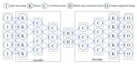
Skin lesion segmentation is the task of identifying and segmenting regions of the skin that are affected by a lesion. This is typically done using a binary classification approach, where each pixel in the input image is classified as either lesion or non-lesion. To use the DCIGN architecture for skin lesion segmentation, we need to modify the decoder to output a binary mask instead of a reconstructed image. This can be done by adding an additional convolutional layer to the decoder with a single output channel and a sigmoid activation function. The layer's output is the likelihood that each input pixel is of the lesion class. A binary cross-entropy loss function is utilised to train the DC-IGN architecture by comparing the predicted binary mask to the ground truth mask. It is common practice to build the ground truth mask by manually labeling each pixel of the input image as lesion or non-lesion. The DCIGN segmentation method is listed in Table 4. Figure 2 depicts the core components of the DCIGN architecture: an encoder, a decoder, and an inverted graphics module. Features are extracted and reconstructed with the help of the convolutional auto encoder and decoder, two common CNN components. While doing segmentation, the inverse graphics module is utilized to create a 3D representation of the input image. Typically, the encoder will consist of several convolutional layers, each of which will be observed by a non-linear initiation function like ReLU. The encoder is responsible for generating the 3D representation by extracting high-level characteristics from the input image. Typically, the decoder will have many deconvolutional layers, each of which will be followed by a non-linear activation function. The purpose of the decoder is to reconstruct the input image from the 3D representation. The inverse graphics module is responsible for generating the 3D representation of the input image. It typically consists of a series of 3D convolutional layers, each followed by a non-linear activation function. The output of the inverse graphics module is a 3D representation of the input image, which is then used to perform segmentation
Table 4. Segmentation algorithm of DCIGN
|
Input: Preprocessed image. Output: DCIGN segmented outcome. |
|
Step 1: The input figure is supplied into the DCIGN model. Step 2: Encoder: The encoder uses a series of convolutional layers to analyze the input image for useful information. To make the model non-linear, the output of each convolutional layer is processed by the ReLU activation function. Step 3: Max-pooling: Max-pooling is used after each convolutional layer to reduce the spatial dimensions of the feature maps. Step 4: Decoder: The decoder consists of multiple deconvolutional layers to reconstruct the image with a segmentation mask. The output of each deconvolutional layer is also passed through a ReLU activation function. Step 5: Skip Connections: Placing skip connections between the encoder and decoder helps increase segmentation precision. At similar spatial resolution, the feature maps from the encoder and the decoder are joined together. Step 6: Output: The output of the DCIGN model is a binary mask that segments the skin lesion from the surrounding skin. Step 7: Loss Function: Combining the binary cross-entropy loss with the Dice loss, this loss function is used to train the DCIGN model. The Dice loss quantifies the degree to which the expected and ground-truth segmentation masks overlap, whereas the binary cross-entropy loss quantifies the difference between the two. |
Convolutional auto encoder: The encoder is a CNN that processes the input image and extracts high-level features. Multi-convolutional layers observed by a non-linear activation function like ReLU are a common component. Let X be the input image and let We and be be the weight matrix and bias vector of the kth convolutional layer in the encoder, respectively.
Figure 2. DCIGN architecture for skin lesion segmentation
Then, the output of the kth convolutional layer can be written as:
$Z_e^k=f_e\left(W_e^k * Z_e^{\{k-1\}}+b_e^k\right)$ (1)
where, * denotes the convolution operation, $Z_e^{k-1}$ is the output of the (k-1) th convolutional layer, and fe is the activation function. The final output of the encoder is a feature map $Z_e^K$, where K is the number of convolutional layers in the encoder.
Decoder: The decoder is a CNN that reconstructs the output image from the feature map generated by the encoder. It is typically composed of several deconvolutional layers, each one followed by a non-linear initiation function.
Let $Z_d^{k-1}$ be the output of the (k-1) th deconvolutional layer and let Wd and bd be the weight matrix and bias vector of the kth deconvolutional layer in the decoder, respectively. Then, the output of the kth deconvolutional layer can be written as:
$Z_d^k=f_d\left(W_d^k * Z_d^{k-1}+b_d^k\right)$ (2)
where, * denotes the transposed convolution operation. The final output of the decoder is the reconstructed image, denoted as X', which is generated by the last deconvolutional layer.
Table 5. Optimal parameter tuning of DCIGN
|
Layer Type |
Output Size |
|
Input Image |
224×224×3 |
|
Convolutional + ReLU |
112×112×32 |
|
Convolutional + ReLU |
56×56×64 |
|
Hidden Skip Connections |
28×28×64 |
|
Convolutional + ReLU |
56×56×64 |
|
Convolutional + ReLU |
112×112×32 |
|
Output |
224×224×3 |
|
Optimizer |
Adam |
|
Regularization |
weight decay |
|
Number of Epochs |
1000 |
|
Batch Size |
64 |
|
Learning Rate |
1e-6 to 1e-2 |
|
Loss Function |
Cross-Entropy |
Inverse Graphics Module: The inverse graphics module is used to generate a 3D representation of the input image, which is then used to perform segmentation. Several 3D convolutional layers are resulted by a non-linear activation function in most implementations. Let Vk-1 be the output of the (k-1) th 3D convolutional layer and let Wv and bv be the weight matrix and bias vector of the kth 3D convolutional layer in the inverse graphics module, respectively. Then, the output of the kth 3D convolutional layer can be written as:
$V^k=f_v\left(W_v^k * V^{k-1}+b_v^k\right)$ (3)
where, * denotes the 3D convolution operation. The final output of the inverse graphics module is a 3D representation of the input image, denoted as R, which is generated by the last 3D convolutional layer. Table 5 shows the optimal design parameters of DCIGN, which are tuned to give the best segmentation performance.
3.3 HDKN feature extraction
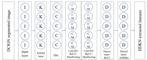
Figure 3. Feature extraction architecture of HDKN
A HDKN is a type of neural network architecture that can be utilized for feature extraction from segmented skin lesion images. The HDKN combines the Kohonen self-organizing map (KSOM) with deep learning techniques to create a hybrid network that can extract useful features from images. Figure 3 shows the feature extraction based HDKN architecture. Table 6 shows the feature extraction algorithm of HDKN. The KSOM is an unsupervised learning algorithm that is used to cluster data based on similarities in their feature vectors. The algorithm is based on a competitive learning process, where each neuron in the network is assigned a weight vector that is used to represent a region in the input space. During training, the input data is presented to the network, and the neuron with the close weight vector is selected as the winner. The weights of the winning neuron are then adjusted to move closer to the input data. This process is repeated for multiple iterations until the weight vectors converge to a stable configuration. The KSOM layer is responsible for clustering the input data based on similarities in their feature vectors. The output of the KSOM layer is a set of feature maps, where each map represents a cluster of input data that have similar features. their feature vectors. It consists of a set of neurons placed in a two-dimensional grid. The input data is presented to the network, and the neuron with the closest weight vector is selected as the winner. The weights of the winning neuron are then informed to move closer to the input data. The update rule can be expressed as:
$w(t+1)=w(t)+\alpha(t)(x-w(t))$ (4)
where, w(t) is the weight vector of the winner neuron at time t, x is the input data, α(t) is the learning rate at time t, and t is the current iteration. The learning rate is typically decreased over time to allow the network to converge to a stable configuration. One common way to decrease the learning rate is to use a decaying function:
$\alpha(t) =\alpha(0) * \exp (-t / \tau)$ (5)
where, α(0) is the initial learning rate, τ is the time constant, and t is the current iteration.
The output of the KSOM layer is a set of feature maps, where each map represents a cluster of input data that have similar features. The CNN layer oversees extracting high-level features from the input data. Several convolutional and pooling layers are used, followed by one or more fully connected layers to complete the layer. High-level features are generated by the CNN layer and utilized for further processing. The KSOM layer is the first to see the input data during training, and it uses similarity in the features to group the data into groups. High-level features are extracted from the clustered data using the KSOM layer's output, which is passed into the CNN layer. During training, the complete network is subjected to supervised learning, during which the loss function is tuned to reduce the gap stuck between the predicted and ground features. Table 7 shows the optimal design parameters of HDKN model, which are tuned to give the best feature extraction performance.
Table 6. Feature extraction algorithm of HDKN
|
Input: DCIGN segmented image. Output: HDKN extracted features. |
|
Step 1: The input skin lesion images are preprocessed to obtain feature maps, where each input pixel is labeled as lesion or non-lesion. Step 2: KSOM layer: The segmented images are shown to the KSOM layer, which is made up of neurons organized in a two-dimensional grid. This layer is responsible for recognizing objects in images. Input data have the same number of dimensions as the weight vector that is associated with each neuron. Step 3: Extracted data clusters (EDC): The KSOM layer clusters the pixels based on similarities in their feature vectors. The output of the KSOM layer is a set of feature maps, where each map represents a cluster of pixels that have similar features. Step 4: After that, the feature maps are sent into the CNN layer, which pulls high-level features from the data that has been clustered together. In most cases, the CNN layer is created up of numerous convolutional and pooling layers, which are then followed by one or more fully connected layers. Step 5: Training: The entire network is trained using a supervised learning approach, where the loss function is optimized to minimize the variation between the expected features and the ground features. |
Table 7. Optimal parameter tuning of DCIGN
|
Layer Type |
Output Size |
|
Input Image |
224×224×3 |
|
Input layer |
224×224×3 |
|
KSOM layer |
120×120 |
|
EDC layer |
100×100 |
|
Convolutional + ReLU |
55×55 |
|
MaxPooling |
5×5 |
|
Convolutional + ReLU |
40×40 |
|
MaxPooling |
3×3 |
|
Dense 1+ ReLU |
1×37460 |
|
Dense 2 + SoftMax |
1×1478 |
|
Output |
1×1478 |
|
Optimizer |
Adam |
|
Regularization |
weight decay |
|
Number of Epochs |
1000 |
|
Batch Size |
64 |
|
Learning Rate |
1e-6 to 1e-2 |
|
Loss Function |
Cross-Entropy |
3.4 SPOA feature selection
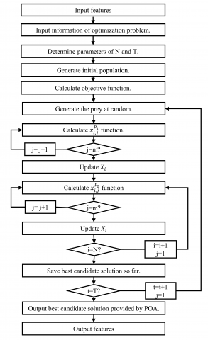
The SPOA algorithm is a meta-heuristic algorithm that uses a population of pelicans to search for the optimal feature subset for a machine learning problem. The algorithm is based on social behaviour of pelicans in nature, where they follow each other in search of food. Table 8 shows the optimal design parameters of SPOA, which are tuned to give the best feature selection performance. Figure 4 shows the feature selection process of SPOA block diagram. Table 9 presents the algorithm of SPOA. The algorithm searches for the optimal solution to a given problem by following a set of movement rules that mimic the flocking behavior of pelicans.
Figure 4. Optimal feature selection process using SPOA
Table 8. Optimal parameter tuning of SPOA
|
Hyperparameter |
Typical Range |
|
Input feature size |
1×1478 |
|
Population Size |
50 to 100 or more |
|
Inertia Weight |
0.1 to 1.0 |
|
Acceleration Constants |
1.0 to 2.0 |
|
Cognitive Coefficient |
1.0 to 2.0 |
|
Social Coefficient |
1.0 to 2.0 |
|
Maximum Iterations |
100 to 1000 or more |
|
Neighborhood Topology |
Global, Ring. |
|
Constriction Factor |
0.5 to 1.0 |
|
Stopping Criteria |
Threshold |
|
output feature size |
1×504 |
Initialization: Let N be the population size and let P={p1, p2, ..., pN} be the set of pelicans. Each pelican represents a potential solution to the optimization problem, where the solution is represented as a vector of binary values xi, i=1, 2, ..., d, where d is the dimension of the problem.
Evaluation: The fitness function f(p) is used to evaluate the quality of each pelican p in the population. The fitness function is typically based on HDKN, and it measures the performance of the algorithm using the selected features. The fitness value is a real number that indicates how well the pelican performs on the optimization problem.
Movement: The pelicans in the population move in search of a better solution by following a set of movement rules that mimic the flocking behavior of pelicans. The movement rules include attraction to the best pelican and avoidance of the worst pelican in the population. The movement of the pelican is defined by the position vector x and the velocity vector v, where vij represents the velocity of pelican i in the j-th dimension. The position and velocity of each pelican are updated at each iteration according to the following equations:
$\begin{aligned} & v_{i j}(t+1)=w * v_{i j}(t)+c 1 * \operatorname{rand}(x) *\left(p_{\text {besti }}, j(t)-x_{i j}(t)\right)+c 2 * \operatorname{rand}(x) *\left(g_{\text {best } j}(t)-x_{i j}(t)\right) x_{i j}(t+1) =x_{i j}(t)+v_{i j}(t+1) \end{aligned}$ (6)
where, w is the inertia weight, c1 and c2 are the acceleration constants, rand () is a random number between 0 and 1, pbesti is the personal best position of pelican i, and gbest is the global best position in the population.
Update: After each iteration, the population is updated based on the movement rules. The bird with the greatest fitness score becomes the "global best pelican," or "gbest," and the others all begin to follow its lead. To keep the pelican population stable, the least fit bird is periodically replaced with a randomly produced new bird.
Termination: When a termination condition is reached, such as a maximum number of iterations or convergence of the fitness values, the SPOA stops.
Selection: The final solution is selected based on the pelican with the highest fitness value in the population.
Table 9. Optimal feature selection algorithm using SPOA
|
Input: HDKN extracted features. Output: SPOA selected features. |
|
Step 1: Initialization: The SPOA algorithm starts by initializing a population of pelicans, each representing a potential solution to the feature selection problem. The population size is defined by the user. Step 2: Evaluation: Each pelican in the population is calculated using a fitness function that measures the quality of the solution. Step 3: Movement: The pelicans in the population move in search of a better solution by following a set of movement rules. Step 4: Update: After each iteration, the population is updated by applying the movement rules. A new pelican is randomly generated to maintain the population size. Step 5: Termination: The SPOA algorithm terminates when a stopping criterion is met. Step 6: Selection: The final solution is selected based on the pelican with the highest fitness value. |
3.5 DENM classifier
The DENM is a type of recurrent neural network that has a simple and efficient training algorithm. It consists of a fixed, randomly initialized sparse connectivity structure of recurrent nodes, and a set of input and output nodes. The output of a DENM is a nonlinear function of its current and past inputs and hidden state. Figure 5 shows the DENM classifier block diagram. Table 10 presents the algorithm steps of DENM for skin cancer classification. Table 11 shows the optimal design parameters of DENM model, which are tuned to give the best classification performance. The mathematical analysis of a DENM involves the following steps.
Initialization of the DENM: The state of the network at time step t is represented by the vector x(t)=[x1(t), x2(t), ..., xn(t)]T, where n is the number of hidden nodes. The input at time t is denoted by u(t)=[u1(t), u2(t), ..., um(t)]T, where n is the number of input nodes. The output at time t is given by y(t)=[y1(t), y2(t), ..., yp(t)]T, where p is the number of output nodes. The connectivity matrix of the DENM is represented by W=[wij], where wij is the weight of the joining from node j to node i. The input weight matrix is represented by $W_{i n}=\left[w_{{i n}_j}\right]$, where $w_{{in}_j}$ is the weight of the joining from input node j to hidden node i. The output weight matrix is represented by $W_{\text {out }}=\left[w_{\text {out }_j}\right]$, where $w_{{o u t}_j}$ is the weight of the joining from hidden node j to output node i. The initial state of the DENM is set to x(0)=0. The input and output weight matrices are randomly initialized.
Dynamics of the DENM: The dynamics of the DENM are described by the following equation:
$x(t)=f\left(W x(t-1)+W_{i n} u(t)\right)$ (7)
where, f is a nonlinear activation function, such as the hyperbolic tangent function. The output of the DENM is given by:
$y(t)=W_{\text {out }} x(t)$ (8)
Figure 5. Classification model of DENM
The DENM has a "reservoir" of hidden nodes that are randomly initialized and fixed throughout training. The weights between the hidden nodes form a sparse, random connectivity structure. The input weights and output weights are learned during training. The output weights of the DENM are trained using a linear regression algorithm. Given a set of input-output pairs {(u(t), d(t))}, where d(t) is the desired output at time t, the output weights are computed using the following equation:
Wout $=\left(X^T R+\right.$ beta $\left.* I\right)-X^T R_D$ (9)
where, X is a matrix of the hidden node activations, R is the regularization matrix, beta is the regularization parameter, I is the identity matrix, and D is a matrix of the desired outputs. The performance of the ESN is evaluated on a separate test set of input-output pairs. The output of the DENM is compared to the desired output using a suitable error metric, such as the mean squared error.
Table 10. Skin cancer classification algorithm of DENM
|
Input: SPOA selected features. Output: Classified cancer type. |
|
Step 1: Initialization: Randomly initialize the weights of the input-to-hidden connections based on SPOA features, the hidden-to-hidden connections, and the hidden-to-output connections. These weights are typically drawn from a Gaussian distribution. Step 2: Define the network structure: Specify the number of hidden, inputs, and output nodes, and the connectivity pattern between them. In the case of a DENM, the input layer receives the input data, the hidden layer comprises of many recurrent nodes, and the output layer produces the network's predictions. Step 3: Forward pass: For each input example in the training set, feed the input through the network and compute the network's output. During this step, the hidden layer of the DENM is updated based on the input and the previous hidden layer state. The output is computed by multiplying the hidden layer state by the output weights and passing it through a nonlinear activation function. Step 4: Calculate error: Compare the network's output to the true target values for the input example, and calculate the error using a suitable loss function, such as mean squared error or cross-entropy loss. Step 5: Backward pass: Propagate the error backwards through the network using the chain rule of calculus, to update the weights of the connections. This involves computing the gradients of the weights with respect to the error, and using gradient descent or a similar optimization algorithm to update the weights in the direction that reduces the error. Step 6: Repeat steps 3-5: Continue feeding input examples through the network, computing the output, calculating the error, and updating the weights, until the error on the training set reaches a satisfactory level. Step 7: Test the model: Use the trained network to make predictions on a separate test set of input examples and evaluate the model's performance on this set. This step is important to ensure that the model generalizes well to new data and resulted in effective skin cancer type. |
Table 11. Optimal parameter tuning of DENM
|
Hyperparameter |
Typical Range |
|
Input Layer |
1×504 |
|
reservoir |
504×504 |
|
Output size |
1×8 |
|
Optimizer |
Adam |
|
Regularization |
weight decay |
|
Number of Epochs |
1000 |
|
Batch Size |
64 |
|
Learning Rate |
1e-6 to 1e-2 |
|
Loss Function |
Cross-Entropy |
This section gives the complete performance analysis of HOS-Net. Further, the performance of HOS-Net is compared with other segmentation, classification models using same ISIC-2019 dataset. Various segmentation and classification metrics are used to evaluate the performance.
4.1 Dataset
International Skin Imaging Collaboration (ISIC) Challenge created a massive collection of skin lesion images, which has been made accessible to the public and given the name ISIC-2019. To further study and improve CAD tools for melanoma, a collection of patient records was compiled. For the ISIC-2019 dataset, researchers gathered a total of 25,331 images of skin lesions from various sources, such as hospitals, clinics, and even people's personal phones. There are a total of eight different forms of skin cancer: Merkel cell carcinoma (MEL), squamous cell carcinoma (SCC), basal cell carcinoma (BCC), melanocytic nevus (NV), benign keratosis (BKL), actinic keratosis (AKIES), vascular lesion (VASC), and dermatofibroma (DF). Each image in the collection is accompanied with ground-truth annotations like lesion segmentation masks and diagnostic labels. A group of board-certified dermatologists rendered the diagnosis of benign or malignant for each lesion. In addition to raw image data and annotations, the ISIC-2019 dataset also includes precomputed image characteristics including color histograms, texture features, and wavelet-based features. This means these characteristics were used to train ML models even when the source images are unavailable.
4.2 Experimental setup
Utilization a GPU-enabled system with NVIDIA CUDA support to take advantage of GPU acceleration. Set up the software environment using Anaconda to manage the Python environment and package dependencies. Split the dataset into training, validation, and test sets. Implement k-fold cross-validation to ensure robust evaluation of the model's performance. Setting of hyperparameters, including learning rate, batch size, number of epochs, dropout rate, and weight decay, using cross-validation for optimal values. Utilization of the GPU for accelerated training by installing the GPU-supported version of TensorFlow and Keras. Used the Adam optimizer with the chosen learning rate and the appropriate loss function for the specific task (e.g., categorical_crossentropy for multi-class classification). Presented the results of the experiments, including accuracy scores, confusion matrices, and learning curves. Analyzed the impact of different hyperparameters on the model's performance. Evaluated the model's performance using metrics like accuracy, precision, recall, and F1-score on a separate test dataset.
4.3 Evaluation metrics
Accuracy: It is the proportion of correctly classified samples out of the total number of samples in the dataset. It measures how well the classifier predicts all classes.
Accuracy $=\left(\frac{(T P+T N)}{(T P+T N+F P+F N)}\right)$ (10)
Precision: It is the proportion of correctly predicted positive samples (true positives) out of all the samples predicted as positive (true positives + false positives). It measures how well the classifier avoids misclassifying negative samples as positive.
Precision $=\left(\frac{(T P)}{(T P+F P)}\right)$ (11)
Recall: It is, also known as true positive rate, is the proportion of correctly predicted positive samples (true positives) out of all the actual positive samples (true positives + false negatives). It measures how well the classifier identifies positive samples.
Recall $=\left(\frac{(T P)}{(T P+F N)}\right)$ (12)
F1-Score: It is the harmonic mean of precision and recall. It provides a balance between precision and recall and is useful when the class distribution is imbalanced.
$F 1-$ score $=\left(\frac{2 *(T P)}{2 * T P+F P+F N}\right)$ (13)
Specificity: It is the proportion of correctly predicted negative samples (true negatives) out of all the actual negative samples (true negatives + false positives). It measures how well the classifier identifies negative samples.
Specificity $=\left(\frac{T N}{T N+F P}\right)$ (14)
4.4 Cross validation analysis
Cross-validation is a widely used technique in deep learning and machine learning to assess the performance and generalization ability of a model on a limited dataset. In the context of the above multi-class skin cancer classification task, cross-validation helps to obtain a more robust estimate of the model's performance by dividing the data into multiple subsets, training the model on different combinations of these subsets, and evaluating its performance across all subsets. The basic idea behind cross-validation is to split the available dataset into several parts, or "folds," and then iteratively train and test the model on different combinations of these folds. The original dataset is divided into K subsets (folds) of approximately equal size. The value of K is determined based on the available data size and computational resources. Common choices for K are 5 to 10. For each fold in the K subsets, the model is trained on K-1 folds and tested on the remaining fold. This process is repeated K times, ensuring that each fold serves as the test set once, while the other K-1 folds are used for training. Cross-validation can also be used for hyperparameter tuning. By running cross-validation for different combinations of hyperparameters (e.g., learning rate, batch size, number of epochs), you can select the optimal set of hyperparameters that result in the best average performance across all folds.
Statistical tests, such as the paired t-test, are essential tools in data analysis and hypothesis testing. The paired t-test is a parametric statistical test used to compare the means of two related groups or conditions. It is called "paired" because the data points are paired, meaning each observation in one group is related to a corresponding observation in the other group. This pairing is crucial when comparing the two conditions, as it helps control for individual differences and reduces variability. The simulation results show that, the proposed HOS-Net resulted in 0.47% error rate in segmentation, and 0.57% error rate in classification.
4.5 Segmentation performance evaluation
Figure 6 shows the skin cancer segmentation outcomes of various methods. Here, the proposed HOS-Net resulted in accurate segmentation outcome as compared to DenseNet201 [14], CNN-GOA [15], InSiNet [18], ESRGAN [21]. One of the main drawbacks of DenseNet201 [14] is its high computational cost, which makes it challenging to deploy the model on resource-constrained devices or in real-time applications. Another limitation is its susceptibility to overfitting, especially when trained on small datasets. The CNN-GOA [15] model relies on manual selection of the optimal segmentation threshold, which can be subjective and time-consuming. Additionally, the model may struggle with segmentation of lesions with complex shapes or irregular boundaries. The InSiNet [18] model is relatively complex, which can make it challenging to train and optimize. It also requires a large amount of training data to achieve optimal performance. The ESRGAN [21] introduce artifacts or distortions in the images, which can affect the accuracy of lesion segmentation. Additionally, the model can be computationally expensive, which can limit its practical applications. Table 12 compares the segmentation performance estimations of various segmentation methods. Here, the proposed HOS-Net resulted in superior performance than conventional methods such as DenseNet201 [14], CNN-GOA [15], InSiNet [18], ESRGAN [21], MLR-CNN [12], and AlexNet [40] for all performance metrics.
Table 13 shows the percentage of improvements of proposed HOS-Net over conventional methods presented in Table 12. Here, the proposed HOS-Net method has increased segmentation accuracy (SACC) by 7.10%, segmentation precision (SPR) by 8.52%, segmentation recall (SRE) by 1.61%, segmentation F1-score (SF1) by 7.19%, segmentation sensitivity (SSEN) by 1.59%, and segmentation specificity (SSPE) by 21.00% as compared to the DenseNet201 [14]. Then, the proposed HOS-Net method has increased SACC by 4.61%, SPR by 8.26%, SRE by 0.79%, SF1 by 6.82%, SSEN by 2.40%, SSPE by 20.51% as compared to the CNN-GOA [15]. Then, the proposed HOS-Net method has increased SACC by 7.36%, SPR by 8.39%, SRE by 0.58%, SF1 by 7.72%, SSEN by 2.15%, SSPE by 22.77% as compared to the InSiNet [18]. Then, the proposed HOS-Net method has increased SACC by 6.59%, SPR 7.11%, SRE by 1.57%, SF1 by 6.27%, SSEN by 1.80%, SSPE by 21.43% as compared to the ESRGAN [21]. Then, the proposed HOS-Net method has increased SACC by 8.42%, SPR by 9.79%, SRE by 0.94%, SF1 by 6.84%, SSEN by 1.85%, SSPE by 22.23% as compared to the MLR-CNN [12]. Finally, the proposed HOS-Net method has increased SACC by 3.53%, SPR by 0.79%, SRE by 1.32%, SF1 by 1.67%, SSEN by 0%, SSPE by 0% as compared to the AlexNet [40].
AUC-ROC allows for a fair and comprehensive comparison of different classifiers or models on the same task. It is especially helpful when you have multiple models trained on the same dataset and want to determine which one performs better. n situations where the classes in the dataset are imbalanced, accuracy alone may not provide a complete picture of a classifier's performance. AUC-ROC considers the trade-off between sensitivity (true positive rate) and specificity (true negative rate), making it suitable for imbalanced datasets.
Figure 6. Skin cancer segmentation outcomes of various methods. (a) input image. (b) DenseNet201 [14]. (c) CNN-GOA [15]. (d) InSiNet [18]. (e) ESRGAN [21]. (f) proposed binary mask. (g) proposed colour segmented region
Table 12. Segmentation performance estimation of various methods
|
Method |
SACC (%) |
SPR (%) |
SRE (%) |
SF1 (%) |
SSEN (%) |
SSPE (%) |
|
DenseNet201 [14] |
93.21 |
91.23 |
97.54 |
92.89 |
98.43 |
82.64 |
|
CNN-GOA [15] |
95.43 |
91.45 |
98.34 |
93.21 |
97.65 |
82.98 |
|
InSiNet [18] |
92.98 |
91.34 |
98.54 |
92.43 |
97.89 |
81.45 |
|
ESRGAN [21] |
93.65 |
92.43 |
97.58 |
93.69 |
98.01 |
82.35 |
|
MLR-CNN [12] |
92.07 |
90.18 |
98.19 |
93.19 |
98.18 |
81.81 |
|
AlexNet [40] |
96.42 |
98.23 |
97.82 |
97.93 |
98.72 |
86.85 |
|
Proposed HOS-Net |
99.83 |
99.01 |
99.12 |
99.57 |
98.94 |
87.12 |
Table 13. Percentage of improvements of Table 12
|
Method |
SACC (%) |
SPR (%) |
SRE (%) |
SF1 (%) |
SSEN (%) |
SSPE (%) |
|
DenseNet201 [14] |
7.10 |
8.52 |
1.61 |
7.19 |
0.79 |
0.41 |
|
CNN-GOA [15] |
4.61 |
8.26 |
0.79 |
6.82 |
0.24 |
1.84 |
|
InSiNet [18] |
7.36 |
8.39 |
0.58 |
7.72 |
0.12 |
1.10 |
|
ESRGAN [21] |
6.59 |
7.11 |
1.57 |
6.27 |
0.17 |
0.65 |
|
MLR-CNN [12] |
8.42 |
9.79 |
0.94 |
6.84 |
0.55 |
6.16 |
|
AlexNet [40] |
3.53 |
0.79 |
1.32 |
1.67 |
0.22 |
0.31 |
4.6 Classification performance evaluation
Figure 7 shows the measurement of area under the ROC curves (AUC) of various methods. Here, receiver operating characteristic curve (ROC) is measured for various thresholds of false positive rate. Further, the ROC region is mapped for true positive rate region to the false positive rate region. Here, the conventional ViT [37] resulted in AUC-ROC value as 0.750, MuSClD [28] resulted in AUC-ROC value as 0.824, and DLCNN [40] resulted in AUC-ROC value as 0.847. But, the proposed HoS-Net resulted in higher AUC-ROC values, i.e., 0.946, which is higher as compared to existing methods.
Figure 7. AUC-RoC curves of various methods
Table 14 compares the classification performance of various SLDC methods. Here, the proposed HOS-Net resulted in improved skin cancer classification performance as compared to conventional ASRGS-OEN [25], WT-DRNNet [34], ORACM [35], ViT [37], MuSClD [28], and DLCNN [40]. Table 15 shows the percentage of improvements by proposed HOS-Net in comparison with existing methods presented in Table 14. Here, the proposed HOS-Net method has increased accuracy by 2.90%, precision by 3.87%, recall by 1.63%, f1-Score by 2.10%, sensitivity by 1.49%, and specificity by 0.87% as compared to the ASRGS-OEN [25]. Then, the proposed HOS-Net method has increased accuracy by 3.85%, precision by 1.56%, recall by 1.38%, f1-Score by 1.39%, sensitivity by 0.33%, and specificity by 1.36% as compared to WT-DRNNet [34]. Then, the proposed HOS-Net method has increased accuracy by 3.04%, precision by 1.51%, recall by 1.03%, f1-Score by 1.77%, sensitivity by 2.00%, and specificity by 2.25% as compared to the ORACM [35]. Then, the proposed HOS-Net method has increased accuracy by 5.07%, precision by 0.80%, recall by 0.92%, f1-Score by 1.35%, sensitivity by 0.63%, and specificity by 1.69% as compared to the ViT [37]. Then, the proposed HOS-Net method has increased accuracy by 3.87%, precision by 1.49%, recall by 0.72%, f1-Score by 1.40%, sensitivity by 0.97%, specificity by 1.03% as compared to the MuSClD [28]. Finally, the proposed HOS-Net method has increased accuracy by 2.81%, precision by 0.91%, recall by 1.46%, f1-Score by 1.66%, sensitivity by 0%, specificity by 0% as compared to the DLCNN [40].
4.7 Computational time estimation
Table 16 compares the computational time (seconds) estimation of various segmentation methods. Here, the proposed HOS-Net resulted in reduced computational time as compared to other segmentation methods. Here, the proposed HOS-Net reduced computation time by -40.23%, -40.13%, -31.25%, -24.10%, -14.39%, -6.70% as compared to existing DenseNet201 [14], CNN-GOA [15], InSiNet [18], ESRGAN [21], MLR-CNN [12], and AlexNet [40] methods. Table 17 compares the computational time (seconds) estimation of various classification methods. Here, the proposed HOS-Net reduced computation time by -32.36 %, -27.69 %, -24.49 %, -11.59 %, -17.72 %, -25.24 % as compared to existing ASRGS-OEN [25], WT-DRNNet [34], ORACM [35], ViT [37], MuSClD [28], and DLCNN [40] methods.
Table 14. Classification performance estimation of various methods
|
Method |
Accuracy (%) |
Precision (%) |
Recall (%) |
F1-Score (%) |
Sensitivity (%) |
Specificity (%) |
|
ASRGS-OEN [25] |
96.33 |
95.43 |
97.65 |
97.51 |
98.53 |
99.13 |
|
WT-DRNNet [34] |
95.45 |
97.60 |
97.89 |
98.19 |
99.67 |
98.65 |
|
ORACM [35] |
96.20 |
97.65 |
98.23 |
97.82 |
98.03 |
97.79 |
|
ViT [37] |
94.34 |
98.34 |
98.34 |
98.23 |
98.37 |
98.33 |
|
MuSClD [28] |
95.43 |
97.67 |
98.54 |
98.18 |
99.03 |
98.98 |
|
DLCNN [40] |
96.42 |
98.23 |
97.82 |
97.93 |
99.15 |
99.12 |
|
Proposed HOS-Net |
99.13 |
99.13 |
99.25 |
99.56 |
99.21 |
99.14 |
Table 15. Percentage of improvements of Table 14
|
Method |
Accuracy (%) |
Precision (%) |
Recall (%) |
F1-Score (%) |
Sensitivity (%) |
Specificity (%) |
|
ASRGS-OEN [25] |
2.90 |
3.87 |
1.63 |
2.10 |
1.15 |
0.48 |
|
WT-DRNNet [34] |
3.85 |
1.56 |
1.38 |
1.39 |
1.64 |
0.87 |
|
ORACM [35] |
3.04 |
1.51 |
1.03 |
1.77 |
0.34 |
0.55 |
|
ViT [37] |
5.07 |
0.80 |
0.92 |
1.35 |
0.67 |
0.66 |
|
MuSClD [28] |
3.87 |
1.49 |
0.72 |
1.40 |
0.12 |
0.14 |
|
DLCNN [40] |
2.81 |
0.91 |
1.46 |
1.66 |
0.06 |
0.02 |
Table 16. Computational time (seconds) estimation of various segmentation methods
|
DenseNet201 [14] |
CNN-GOA [15] |
InSiNet [18] |
ESRGAN [21] |
MLR-CNN [12] |
AlexNet [40] |
Proposed HOS-Net |
|
12.514 |
12.484 |
10.87 |
9.847 |
8.73 |
8.01 |
7.473 |
Table 17. Computational time (seconds) estimation of various classification methods
|
ASRGS-OEN [25] |
WT-DRNNet [34] |
ORACM [35] |
ViT [37] |
MuSClD [28] |
DLCNN [40] |
Proposed HOS-Net |
|
15.484 |
14.484 |
13.87 |
11.847 |
12.73 |
14.01 |
10.473 |
Skin cancer is a serious global health concern, and its early detection and diagnosis are crucial for improving the chances of successful treatment and increasing the survival rate of affected individuals. This work introduced the HOS-Net by combining the multiple stages. At first, the dataset augmentation is carried out, which results in a growth in the total amount of images included inside the dataset. After that, the image pre-processing is carried out to standardise the images in the dataset into sizes and data types that are consistent throughout. In addition, DCIGN was created for the purpose of recognising disease-affected regions within images that had already been pre-processed. After that, the HDKN is presented for the purpose of the extraction of disease-specific characteristics that rely on the disease from the segmented image. Additionally, the SPOA selects the most relevant features from the HDKN output features. Last, DENM classifies the various diseases based on their SPOA traits that have been pretrained. The proposed HOS-Net method has increased SACC by 3.53%, SPR by 0.79%, SRE by 1.32%, SF1 by 1.67%, SSEN by 0%, SSPE by 0% as compared to the other segmentation methods. Finally, the proposed HOS-Net method has increased accuracy by 2.81%, precision by 0.91%, recall by 1.46%, f1-Score by 1.66%, sensitivity by 0%, specificity by 0% as compared to other classification methods.
The potential application of HOS-Net in clinical environments offers several promising benefits for the diagnosis and management of skin cancer. HOS-Net can act as a valuable tool to support dermatologists in their decision-making process. By providing additional insights and analysis, it can serve as a second opinion and help dermatologists make more informed decisions about the diagnosis and treatment of skin cancer. With its deep learning capabilities, HOS-Net can process and analyze large datasets of skin lesion images quickly and efficiently. This can streamline the workflow in clinical settings, enabling faster diagnosis and reducing waiting times for patients. HOS-Net's automated analysis can be integrated into telemedicine platforms, allowing for remote consultation and assessment of skin lesions. This can be particularly valuable in rural or underserved areas where access to dermatologists might be limited. HOS-Net's deep learning capabilities can be utilized for longitudinal monitoring of skin lesions over time. By tracking changes in lesion characteristics, it can help in assessing treatment efficacy and disease progression. HOS-Net's deep learning capabilities can be utilized for longitudinal monitoring of skin lesions over time. By tracking changes in lesion characteristics, it can help in assessing treatment efficacy and disease progression.
[1] Ghahfarrokhi, S.S., Khodadadi, H., Ghadiri, H., Fattahi, F. (2023). Malignant melanoma diagnosis applying a machine learning method based on the combination of nonlinear and texture features. Biomedical Signal Processing and Control, 80: 104300. https://doi.org/10.1016/j.bspc.2022.104300
[2] Aguiar Krohling, B., Krohling, R.A. (2023). 1D Convolutional neural networks and machine learning algorithms for spectral data classification with a case study for Covid-19. arXiv e-prints, arXiv-2301. https://doi.org/10.48550/arXiv.2301.10746
[3] Xu, X., Fan, H., Wang, M., Cheng, X., Chen, C. (2022). A Method for Classification of Skin Cancer Based on VisionTransformer. In The International Conference on Natural Computation, Fuzzy Systems and Knowledge Discovery, pp. 210-217. https://doi.org/10.1007/978-3-031-20738-9_25
[4] Tajjour, S., Garg, S., Chandel, S.S., Sharma, D. (2023). A novel hybrid artificial neural network technique for the early skin cancer diagnosis using color space conversions of original images. International Journal of Imaging Systems and Technology, 33(1): 276-286. https://doi.org/10.1002/ima.22784
[5] Sharafudeen, M. (2023). Detecting skin lesions fusing handcrafted features in image network ensembles. Multimedia Tools and Applications, 82(2): 3155-3175. 10.1007/s11042-022-13046-0
[6] Maniraj, S.P., Maran, P.S. (2022). A hybrid deep learning approach for skin cancer diagnosis using subband fusion of 3D wavelets. The Journal of Supercomputing, 78(10): 12394-12409. 10.1007/s11227-022-04371-0
[7] Singh, S.K., Abolghasemi, V., Anisi, M.H. (2022). Skin Cancer Diagnosis Based on Neutrosophic Features with a Deep Neural Network. Sensors, 22(16): 6261. https://doi.org/10.3390/s22166261
[8] Araújo, R.L., Araújo, F.H.D., Silva, R.R.E. (2022). Automatic segmentation of melanoma skin cancer using transfer learning and fine-tuning. Multimedia Systems, 28(4): 1239-1250. https://doi.org/10.1007/s00530-021-00840-3
[9] Reshma, G., Al-Atroshi, C., Nassa, V.K., Geetha, B.T., Sunitha, G., Galety, M.G., Neelakandan, S. (2022). Deep learning-based skin lesion diagnosis model using dermoscopic images. Intelligent Automation & Soft Computing, 31(1).
[10] Ashraf, H., Waris, A., Ghafoor, M.F., Gilani, S.O., Niazi, I.K. (2022). Melanoma segmentation using deep learning with test-time augmentations and conditional random fields. Scientific Reports, 12(1): 3948. https://doi.org/10.1038/s41598-022-07885-y
[11] Krishna, D.M., Sahu, S.K., Raju, G.S. (2021). MLRNet: Skin lesion segmentation using hybrid Gaussian guided filter with CNN. In 2021 5th International Conference on Electronics, Communication and Aerospace Technology (ICECA), Coimbatore, India, pp. 1337-1343. https://doi.org/10.1109/ICECA52323.2021.9676020
[12] Nawaz, M., Mehmood, Z., Nazir, T., Naqvi, R.A., Rehman, A., Iqbal, M., Saba, T. (2022). Skin cancer detection from dermoscopic images using deep learning and fuzzy k-means clustering. Microscopy Research and Technique, 85(1): 339-351. https://doi.org/10.1002/jemt.23908
[13] Bassel, A., Abdulkareem, A.B., Alyasseri, Z.A.A., Sani, N.S., Mohammed, H.J. (2022). Automatic malignant and benign skin cancer classification using a hybrid deep learning approach. Diagnostics, 12(10): 2472. https://doi.org/10.3390/diagnostics12102472
[14] Attique Khan, M., Sharif, M., Akram, T., Kadry, S., Hsu, C.H. (2022). A two-stream deep neural network‐based intelligent system for complex skin cancer types classification. International Journal of Intelligent Systems, 37(12): 10621-10649. https://doi.org/10.1002/int.22691
[15] Thapar, P., Rakhra, M., Cazzato, G., Hossain, M.S. (2022). A novel hybrid deep learning approach for skin lesion segmentation and classification. Journal of Healthcare Engineering, 2022: 1709842. https://doi.org/10.1155/2022/1709842
[16] Mohakud, R., Dash, R. (2022). Skin cancer image segmentation utilizing a novel EN-GWO based hyper-parameter optimized FCEDN. Journal of King Saud University-Computer and Information Sciences, 34(10): 9889-9904. https://doi.org/10.1016/j.jksuci.2021.12.018
[17] Shorfuzzaman, M. (2022). An explainable stacked ensemble of deep learning models for improved melanoma skin cancer detection. Multimedia Systems, 28(4): 1309-1323. https://doi.org/10.1007/s00530-021-00787-5
[18] Reis, H.C., Turk, V., Khoshelham, K., Kaya, S. (2022). InSiNet: a deep convolutional approach to skin cancer detection and segmentation. Medical & Biological Engineering & Computing, 1-20. https://doi.org/10.1007/s11517-021-02473-0
[19] Lakshminarayanan, A.R., Bhuvaneshwari, R., Bhuvaneshwari, S., Parthasarathy, S., Jeganathan, S., Sagayam, K.M. (2022). Skin cancer prediction using machine learning algorithms. In Artificial Intelligence and Technologies: Select Proceedings of ICRTAC-AIT 2020, pp. 303-310. https://doi.org/10.1007/978-981-16-6448-9_31
[20] Afza, F., Sharif, M., Mittal, M., Khan, M.A., Hemanth, D.J. (2022). A hierarchical three-step superpixels and deep learning framework for skin lesion classification. Methods, 202: 88-102. https://doi.org/10.1016/j.ymeth.2021.02.013
[21] Alwakid, G., Gouda, W., Humayun, M., Sama, N.U. (2022). Melanoma detection using deep learning-based classifications. In Healthcare, 10(12): 2481. https://doi.org/10.3390/healthcare10122481
[22] Bindhu, A., Thanammal, K.K. (2023). Segmentation of skin cancer using Fuzzy U-network via deep learning. Measurement: Sensors, 26: 100677. https://doi.org/10.1016/j.measen.2023.100677
[23] Naeem, A., Anees, T., Fiza, M., Naqvi, R.A., Lee, S.W. (2022). SCDNet: A deep learning-based framework for the multiclassification of skin cancer using dermoscopy images. Sensors, 22(15): 5652. https://doi.org/10.3390/s22155652
[24] Kumar, K.A., Vanmathi, C. (2022). Optimization driven model and segmentation network for skin cancer detection. Computers and Electrical Engineering, 103: 108359. https://doi.org/10.1016/j.compeleceng.2022.108359
[25] Alam, T.M., Shaukat, K., Khan, W.A., Hameed, I.A., Almuqren, L.A., Raza, M.A., Aslam, M., Luo, S. (2022). An efficient deep learning-based skin cancer classifier for an imbalanced dataset. Diagnostics, 12(9): 2115. https://doi.org/10.3390/diagnostics12092115
[26] Liu, L., Qi, M., Li, Y., Liu, Y., Liu, X., Zhang, Z., Qu, J. (2022). Staging of skin cancer based on hyperspectral microscopic imaging and machine learning. Biosensors, 12(10): 790. https://doi.org/10.3390/bios12100790
[27] Aljohani, K., Turki, T. (2022). Automatic classification of melanoma skin cancer with deep convolutional neural networks. Ai, 3(2): 512-525. https://doi.org/10.3390/ai3020029
[28] Rashid, J., Ishfaq, M., Ali, G., Saeed, M.R., Hussain, M., Alkhalifah, T., Alturise, F., Samand, N. (2022). Skin cancer disease detection using transfer learning technique. Applied Sciences, 12(11): 5714. https://doi.org/10.3390/app12115714
[29] Kaur, R., GholamHosseini, H., Sinha, R., Lindén, M. (2022). Melanoma classification using a novel deep convolutional neural network with dermoscopic images. Sensors, 22(3): 1134. https://doi.org/10.3390/s22031134
[30] Soujanya, A., Nandhagopal, N. (2023). Automated skin lesion diagnosis and classification using learning algorithms. Intelligent Automation & Soft Computing, 35(1): 676-687. https://doi.org/10.32604/iasc.2023.025930
[31] Kumar, A., Satheesha, T.Y., Salvador, B.B.L., Mithileysh, S., Ahmed, S.T. (2023). Augmented Intelligence enabled Deep Neural Networking (AuDNN) framework for skin cancer classification and prediction using multi-dimensional datasets on industrial IoT standards. Microprocessors and Microsystems, 97: 104755. https://doi.org/10.1016/j.micpro.2023.104755
[32] Albawi, S., Arif, M.H., Waleed, J. (2023). Skin cancer classification dermatologist-level based on deep learning model. Acta Scientiarum. Technology, 45: e61531-e61531. https://orcid.org/0000-0002-9111-1210
[33] Zhou, Y., Koyuncu, C., Lu, C., Grobholz, R., Katz, I., Madabhushi, A., Janowczyk, A. (2023). Multi-site cross-organ calibrated deep learning (MuSClD): Automated diagnosis of non-melanoma skin cancer. Medical Image Analysis, 84: 102702. https://doi.org/10.1016/j.media.2022.102702
[34] Mukadam, S.B., Patil, H.Y. (2023). Skin cancer classification framework using enhanced super resolution generative adversarial network and custom convolutional neural network. Applied Sciences, 13(2): 1210. https://doi.org/10.3390/app13021210
[35] Kanwal, N., Amundsen, R., Hardardottir, H., Janssen, E. A., Engan, K. (2023). Detection and localization of melanoma skin cancer in histopathological whole slide images. arXiv preprint arXiv:2302.03014. https://doi.org/10.48550/arXiv.2302.03014
[36] Gajera, H.K., Nayak, D.R., Zaveri, M.A. (2023). A comprehensive analysis of dermoscopy images for melanoma detection via deep CNN features. Biomedical Signal Processing and Control, 79: 104186. https://doi.org/10.1016/j.bspc.2022.104186
[37] Kollipara, V.H., Kollipara, V.D.P. (2021). Residual Learning Based Approach for Multi-class Classification of Skin Lesion Using Deep Convolutional Neural Network. In International Conference on Cognition and Recongition, pp. 340-351. https://doi.org/10.1007/978-3-031-22405-8_27
[38] Alenezi, F., Armghan, A., Polat, K. (2023). A multi-stage melanoma recognition framework with deep residual neural network and hyperparameter optimization-based decision support in dermoscopy images. Expert Systems with Applications, 215: 119352. https://doi.org/10.1016/j.eswa.2022.119352
[39] Alenezi, F., Armghan, A., Polat, K. (2023). Wavelet transform based deep residual neural network and ReLU based Extreme Learning Machine for skin lesion classification. Expert Systems with Applications, 213: 119064. https://doi.org/10.1016/j.eswa.2022.119064
[40] Krishna, D.M., Sahu, S.K., Raju, G.S. (2022). DTLNet: Deep transfer learning-based hybrid model for skin lesion detection and classification. In 2022 2nd Asian Conference on Innovation in Technology (ASIANCON), Ravet, India, pp. 1-8. https://doi.org/10.1109/ASIANCON55314.2022.9909252