Emir Mustafa Efe*![]() | Veysel Gökhan Böcekçi
| Veysel Gökhan Böcekçi![]()
© 2023 IIETA. This article is published by IIETA and is licensed under the CC BY 4.0 license (http://creativecommons.org/licenses/by/4.0/).
OPEN ACCESS
This study aims to establish an automated system for regulating vehicle speed limits contingent on weather conditions, leveraging deep learning and computer vision methodologies. The advent of advanced vehicle technologies has contributed to escalated traffic density and accident rates. Consequently, there is a growing consensus in accident prevention research literature advocating for the proliferation of electronic monitoring systems. These systems proffer cost-effectiveness by diminishing dependence on field personnel and vehicles. However, existing systems largely establish speed limits based on the roadway and vehicle type, neglecting the impact of weather conditions. The methodology proposed herein employs deep learning models for weather condition detection and image processing techniques for vehicle speed estimation from video data. The Kalman filter is utilized for tracking and speed verification. The constructed system comprises three different cameras, each possessing an individual model. These models exhibit accuracy rates of 99.51%, 99.85%, and 99.60% in weather classification, respectively. Vehicle detection accuracy ranges from 76.46% to 94.67%, with a mean speed estimation error rate of 2.54%. By dynamically modulating speed limits grounded on real-time weather and traffic conditions, this system augments road safety. Furthermore, it provides valuable data on traffic density by recording the quantity of vehicles traversing the relevant highway.
deep learning, Kalman filter, morphological transformations, speed estimation, video processing
1.1 Problem definition
In this study, it is aimed to automatically perform the speed control according to the weather conditions, which is done manually in a few European countries, and it is tried to be suitable for the purpose of the control together with the detection of violations. With electronic monitoring systems, it is aimed to support 24/7 inspection by using less personnel. Thanks to the computer program using image processing methods and deep learning methods, it is aimed to demonstrate that electronic inspections can be made with camera images that can be accessed remotely, without the need for high-tech and costly cameras. In addition, valuable data have been created to be used in different studies with the number and density of vehicles.
With the technological developments in electronic systems, speed limit application is widely used in electronic control systems for vehicles on highways, such as license plate recognition, speed limit control, incorrect lane change control, phone use control while driving, etc. With the increase in the availability and functionality of these systems, drivers try to ensure safer travel by complying with the rules in a conscious and controlled manner.
However, there are problems in the design and use of these electronic systems. While high-tech cameras are sufficient in some regions for speed limit enforcement, in some regions additional speed sensor devices are used due to old technology, lack of infrastructure, faulty planning, etc. The existence of these devices both increases the cost and reduces workforce efficiency as it requires maintenance.
Another issue is that in many European countries, speed limits on highways are determined based on the vehicle type and the highway used. When determining speed limits, weather conditions, which are as important a parameter as the vehicle type and the highway used, are not taken into account. In this case, driving at a speed appropriate to seasonal conditions depends on the driver's discretion and the presence of field supervisory personnel.
Over speed is the speed at which the speed limit exceeded. While speeding is the cause of the majority of fatal accidents, it is also an important factor determines the severity of the accidents. As can be seen in Figure 1 [1], the risk of accident increases as the changes in average speed increase.
Nevertheless, drivers tend to over speed while driving. According to the research conducted in European countries within the scope of the Safe Road Trains for the Environment project [2], 82% of drivers know that excessive speed is an important accident factor, yet more than 70% of them state that they exceed the speed limit. With speed limits not set in a weather-adaptive manner, the risk of accidents will depend on the discretion of drivers found to be over speeding at 70%.
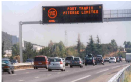
In France a variable speed limit is applied according to the weather conditions. In case of rain and snow or in heavy traffic conditions, the speed limit on highways is reduced from 130 km/h to 110 km/h, and from 90 km/h to 80 km/h on city roads. In case of fog the speed limit is reduced to 50 km/h. As shown in Figure 2 [2], this method takes place manually and remains within the regional scope.
Figure 1. Speed-accident risk graph
Figure 2. Manually changed speed limit in heavy traffic in France
In addition, there are NZLIMITS in New Zealand, USLIMITS in America, QLIMITS, NLIMITS, VLIMITS etc. [2] different applications from other countries. In these applications, appropriate speed limits for highway safety are determined according to different factors such as road characteristics, accident history, number of uses and activities.
1.2 Background
1.2.1 Convolutional Neural Network (CNN)
The CNN method emerged with the development of the concept of artificial intelligence, which was questioned by the Imitation Game [3] test designed by Alan Turing in 1950. The journey of developing deep learning methods commenced in 1943 with McCulloch and Pitts' study [4], which unveiled a logical model of brain functions inspired by the human nervous system. Additionally, in 2012 Krizhevsky and Sutskever's study presented during the ImageNet Large Scale Visual Recognition Challenge [5], marked a significant milestone in advancing deep learning to a foundational level.
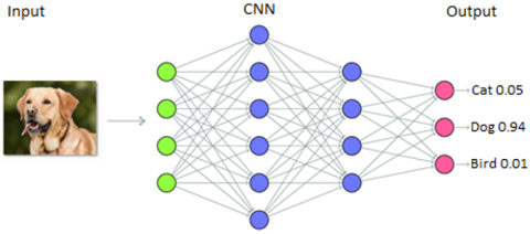
A Sequential Convolutional Neural Network (CNN) is a deep learning architecture characterized by its sequential arrangement of layers. In a Sequential CNN, layers are stacked one after another in a linear fashion, forming a unidirectional flow of data from input to output. Typically, the architecture starts with an input layer and proceeds with a series of convolutional layers for feature extraction, interspersed with pooling layers for spatial downsampling. Following the convolutional and pooling layers, one or more fully connected layers may be added for classification or regression tasks. The simplicity and ease of implementation of Sequential CNNs, make them a popular choice for image-based applications. In Figure 3, the Sequential CNN layer architecture used in this study is given as a visual diagram.
The mathematical expression of the convolution operation [6] is as shown in Eq. (1).
$S(i, j)=(I * K)(i * j)=\sum_m \sum_n I(i+m, j+n) K(m+n)$ (1)
In the equation, S represents the convolution operation output, I represents the input, K kernel and * denotes the convolution operation.
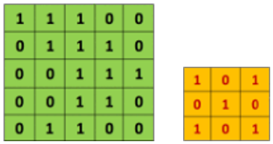
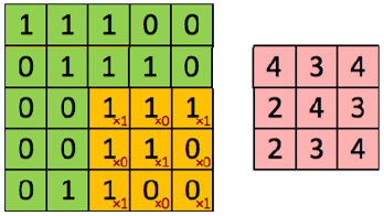
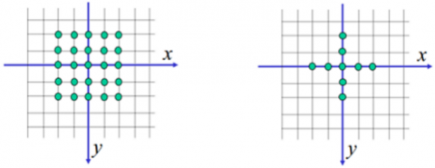
Convolutional Layer. The convolution layer used to determine the properties of the input is the step in which the filters performing the convolution operations are scanned horizontally and vertically in the input. For example, when the image in Figure 4, which consists of 1s and 0s as input, is scanned with the CNN filter given, the output feature map to be obtained is as shown in Figure 5 [7]. Here, while the filter is moved starting from the upper left corner of the sample image, the values between the two matrices are multiplied and the results are summed. The collected results are stored in the feature map. This process is repeated for the elements in each row and column in the visual. Figure 5 shows the final processing of the sample CNN filter in the image. The value 4, which is the (3,3) element of the feature map, is obtained as a result of the following Eq. (2).
$(1 \times 1)+(1 \times 0)+(1 \times 1)+(1 \times 0)+(1 \times 1)+(0 \times 0)+(1 \times 1)+(0 \times 0)+(0 \times 1)=4$ (2)
Figure 3. CNN layer architecture
Figure 4. Input and CNN filter
Figure 5. Filtering and result
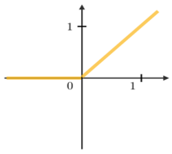
Rectified Linear Unit Layer (ReLU). This layer, which comes after the convolution layers, is the layer where neuron outputs are rectified to become ready for other layers. Negative values in the data coming after the convolution layer are set to zero and are not used during learning. For this reason, the ReLU activation function is often preferred in multilayer neural networks. Thanks to the operations performed in this layer, deep learning accelerates even more. Figure 6 [6] contains example for commonly used activation functions. The mathematical expression of the ReLU function is given in Eq. (3).
$g(x)=\max (0, x)=\begin{aligned} & x, x \geq 0 \\ & 0, x<0\end{aligned}$ (3)
Figure 6. ReLU activation function
Pooling Layer. Pooling layer is the layer where calculations are made in the network architecture. The success of the model created in this layer is calculated and the dimensionality is desired to be reduced. In this way, the required power and features that are determined but will not be used are filtered. There are two different pooling methods: maximum and average pooling. Maximum and average pooling transactions are shown below in Figure 7 [8].
Figure 7. Max and average pooling
Fully-Connected Layer. In this layer, the input image, which passes through the convolution layer and the jointing layer several times and is in the form of a matrix, is converted into a flat vector suitable for the classification layer. Figure 8 [6] shows the process of preparing the neurons emerging after the convolution operations for the classification layer as a single and flat vector in the full connection layer.
Figure 8. Fully-connected layer
Classification Layer. This layer comes after the fully-connected layer and converts the data coming from the neurons into logical values equal to the number of objects to be classified. For example, 1024 neurons entering this layer are output as a 1024×3 weight matrix for 3 different objects. The most commonly used classifier in this layer is softmax. Softmax produces values between 0-1 for each object to be predicted, the object with the value closest to 1 is predicted as the output of the model. Figure 9 shows an example output for the classification process.
Figure 9. Classification
Softmax. It is generally used in the last layer of neural networks, where the probability distribution of n different events is calculated. Its most important advantage is that it can handle multiple classes. Its mathematical expression can be seen in Eq. (4) [6].
$Softmax\left(x_i\right)=\frac{e^{x_i}}{\sum_{j=1}^n e^{x_j}}$ (4)
In this study, deep learning is performed with a database consisting of camera images using the CNN algorithm. The most important reason for choosing CNN as the deep learning algorithm method is that the database preprocessing of the CNN algorithm is much less than other methods and the learning processes are much faster. The weather forecast was taken as the result of the Softmax algorithm as the deep learning output. The model output will be used in weather detection and model queries have been carried out at certain periods. After the weather condition was determined according to the model output, the image processing parameters to be used in the application were updated and the speed limit was determined. Vehicle speed control has been implemented according to appropriate parameters and speed limit.
1.2.2 Morphological transformations
Morphological transformation is an analysis method based on nonlinear operations related to the shape and geometry of features in an image. It is generally used to clean the areas/objects that are desired to be separated in binary images from objects outside the region of interest. During these processes, the configuration element is hovered over the input image. Various mathematical operations are performed according to the pixel value of the image and the value of the configuration element. There are examples of structuring elements in Figure 10 [9].
Figure 10. Structuring element examples
Erosion. Erosion is used to shrink and erode objects in the image. Comparison is made by moving the structuring element pixel by pixel over the image. If the center value of the configuration element corresponds to the value 1 in the visual, and if the visual has a value of 0 under the other 1 values of the configuration element, the visual pixels under the other 1 values of the configuration element are converted to 0. Erosion is used to remove unwanted noise because it reduces peaks and increases the width of 0-pixel regions in the image. Figure 11 [9] shows the image obtained when the erosion process is applied on the first image.
Figure 11. Erosion
Dilation. Dilation is used to enlarge and expand objects in the image. The structuring element is moved pixel by pixel over the image. When the configuration element coincides with a pixel with a value of 1 in the central image, the visual pixel values below the other values are changed to 1. Expansion expands the width of 1-pixel regions in the image, so it can remove negative noise but can also increase unwanted noise. Figure 12 [9] shows the image (b) obtained when the dilation process is applied on the first image (a).
Figure 12. Dilation
Opening. First Erosion and then Dilation is performed on the original image. While the structuring element moves pixel by pixel in the image, it eliminates less valuable pixels in the image and ensures that other regions remain the same. Thus, fine lines, spots and unwanted noise in the image are eliminated. In the 3 images in Figure 13 [9] respectively; original image, 5×5 Opened image, 9x9 Opened image.
Figure 13. Opening
Closing. First Dilation and then Erosion is performed on the original image. The aim of the closing process is to eliminate the gaps by filling them. While the configuration element is moved pixel by pixel in the image, if a 1-valued pixel of the image coincides with the element center, it ensures that the low-value pixels below the other values of the element are converted to 1. In the image in Figure 14 [9], it can be seen that the recesses and gaps in the object are closed as a result of the Closing process.
Figure 14. Closing
1.2.3 Distance calculation
Euchlidean distance is a calculation of between two points. Euclidean distance between points in n-dimensional Euclidean space [10] is given in Eq. (5).
$d_{\text {euc }}$$=\sqrt{\left(p_1-q_1\right)^2+\left(p_2-q_2\right)^2+. .+\left(p_n-q_n\right)^2}$ (5)
where, p and q represent the points in the x and y plane of the coordinates for which the Euclidean distance calculation is made.
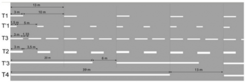
Figure 15. Traffic lines used in France
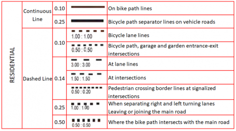
We used lane markings and on-road measurements to automatically calculate the actual distance from the camera image. For this purpose, the T'1 marking method specified in the study [11] and shown in Figure 15 was taken as basis for Camera #4. In addition, as given in Figure 16, according to the guide published by the General Directorate of Highways (KGM) for the cameras in Istanbul [12], the system was calibrated so that the lane lines and intervals on the road in the relevant camera were 3 meters each.
Figure 16. Traffic line characteristics in Turkey
1.2.4 Kalman filter
The Kalman filter [13] was published by R. E. Kalman in 1960 with the aim of extracting useful signal from noisy measurement values. R. E. Kalman used this approach to predict states based on linear dynamical systems in state space format. More generally, the Kalman filter is an algorithm that can predict the next state of a model based on data from the previous state. The biggest reason why this algorithm is called a filter is that it can separate the actual value in the measurements and the noise by optimizing it according to the predictions it makes.
In systems using sensors such as radar, laser and sonar, the Kalman filter is usually only concerned with the position of the target. In general terms, the $Z_k$ measurement vector, H (measurement matrix) and R (covariance matrix) values for tracking the moving object are expressed as in Eq. (6), Eq. (7) and Eq. (8) below [14]. Here, the $B_x$ value is a variant of the position measurement errors and the $v_k$ value is the measurement noise.
$Z_k=H_{x_{t k}}+v_k$ (6)
$H=\left(\begin{array}{ll}1 & 0\end{array}\right)$ (7)
$R=\left(B_x\right)$ (8)
1.3 Related works
Similar studies carried out before are discussed as follows:
In the study by Chowdhury et al. [15], vehicle detection study was carried out with image processing methods. In the study, vehicle detection achieved a 95.08% success rate for the daytime period and 94.10% for the nighttime period.
In the study by Biswas et al. [16], CNN architecture was used for vehicle detection and counting. An average of 96.55% success rate was achieved in the counts made at certain time periods for more than one database. As stated in this study, vehicle counting could not be performed during heavy rain and snowy weather conditions, and it was also reported that the vehicles that changed lanes were counted more than once, since the vehicle count was made according to the vehicles passing in the lane.
In the study conducted by Hsieh et al. [17], the counting efficiency was tried to be increased with shadow filtering and linearity by using image-processing methods during vehicle counting. As a result of the study, it was seen that the vehicle counting success rate was between 92.8% and 94.8% for different cameras.
In the study conducted by Gupte et al. [18], vehicle detection, tracking and classification were performed using image processing methods. As a result of this study, vehicles were detected and tracked with a success rate of 90% in 20 minutes, 15 fps video images and classified as successful with a success rate of 70%.
In the study conducted by Van Pham and Lee [19], vehicle counting was performed using image-processing methods. As a result of the study, the vehicles in a 20-minute image were detected and counted as 98% successful.
In the study conducted by Bhaskar and Yong [20], vehicle counting was performed using image-processing methods. As a result of the study, as a result of the counting made in three different videos, a successful count of 91.26% was achieved.
In the study conducted by Yaghoobi Ershadi et al. [21], vehicle detection in different densities, weather conditions, road type, light intensity and spaces was achieved with approximately 94.02% success.
In the study conducted by Tayara et al. [22], the vehicle counting study from satellite images was carried out with a model prepared using FCRN with a 90.51% success rate.
In the study by Wicaksono et al. [23], vehicle detection was performed using image processing methods and morphological transformations, and approximate vehicle speed estimation was performed. The speed estimation success rate was 87.01%, but it was determined that the system created in this study increased the error rate at high speeds.
In the study by Chu et al. [24], temperature, humidity and weather forecasts were made using SVM architecture. At the end of the study, it was seen that the weather forecast was correct with an average of 76.6%. However, among the 5 weather conditions used in the study, it was observed that the performance was below the general average of 76.6% for rainy and cloudy weather conditions.
In the study by Zhang et al. [25], weather classification was applied using Multi-Core Learning (MKL) with a database consisting of 4000 images. The overall average success rate was 71.39%. In this model, 32% of rainy images were incorrectly classified as snowy.
In the study carried out by Roser and Moosmann [26], forecasts were made for clear, light rainy and heavy rainy weather conditions with the designed SVM model and the success rate was obtained as 85.19%.
Vehicle detection algorithms were created in the study by Luo et al. [27]. As a result of the application, a 92.25% success rate was achieved for vehicle detection.
In the study conducted by Chen et al. [28], as a result of the model created using the Faster R-CNN algorithm, vehicle detection for various types of vehicles was performed with an average success rate of 75.7%.
In this study, all deep learning and image processing operations created run on the CPU on a computer with an Intel® Core™ i7-9750H 2.60GHz CPU [29] processor and 16.0 GB RAM. An interface shown in Figure 17 has been designed to access the cameras and input the operating parameters and settings. While designing this interface, the python software language v3.9.6 [30] and pygt5 library [31] are used. Other auxiliary libraries are cv2 v4.6.0 [32], numpy v1.23.4 [33], pandas v1.5.1 [34], pafy v0.5.5 [35] and tensorflow v2.10.0 [36]. Work flow for this study can be found in Figure 18.
2.1 Dataset
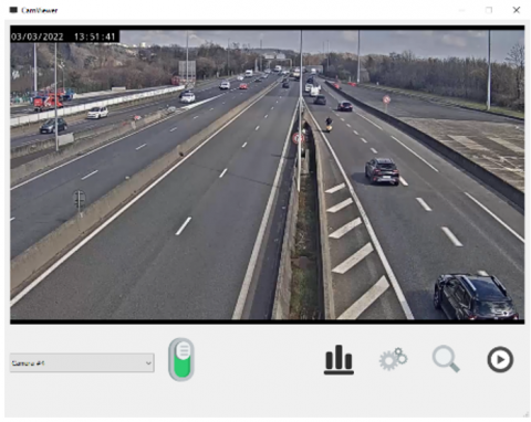
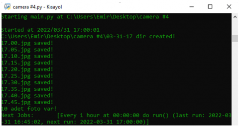
With the software application named SelfDb, which was specially prepared for this study that takes the access links to the specified cameras as input, the camera images with the preferred intervals and parameters were saved in the relevant directory. For this study, a maximum of 10 screenshots were recorded every hour at 5-minute intervals for 24 hours and for 6 months, covering four different weather conditions which snow, rain, fog and normal. Screenshots were 1280×720 resolution and color images. Figure 19 shows the screenshot of the SelfDb application working.
With the SelfDb application, which takes the access links to the specified cameras as input, as given in Table 1, camera images are saved in the relevant directory in accordance with the preferred periods and parameters. Among the cameras identified, there are freeway cameras located in the city of France / Lyon [37], many central and highway cameras in the city of Türkiye / Istanbul [38]. These cameras, which are accessed online from many countries and cities, do not technically require any features, but the image quality, fixed camera structure and access stability make these cameras one step ahead in choosing them. In Figure 20 there are screenshots taken from the traffic density map provided by İBBUYM [38]. There are sample images that can be used for normal, rainy, snowy and foggy weather conditions.
Figure 17. User interface
Figure 18. Application work flow
Figure 19. SelfDb application
Figure 20. Istanbul-various weather conditions
Table 1. Camera list
|
Camera |
Resolution |
fps |
Location |
URL |
|
Camera #4 |
1280×720 |
60 |
Lyon |
www.youtube.com/watch?v=z545k7Tcb5o |
|
Camera #12 |
1920×1080 |
30 |
İstanbul |
uym.ibb.gov.tr/yharita6/ |
|
Camera #13 |
1920×1080 |
30 |
İstanbul |
uym.ibb.gov.tr/yharita6/ |
Table 2. Datasets and demographic structures
|
CNN Model |
Class |
Format |
Original Resolutions |
Pcs |
Process Image Resolutions |
Accuracy |
|
Camera #4.model |
snow (kar) |
.jpg |
1280×720 |
38 |
150×150 |
99.51% |
|
normal |
.jpg |
1280×720 |
1645 |
150×150 |
||
|
fog (sis) |
.jpg |
1280×720 |
468 |
150×150 |
||
|
rain (yagmur) |
.jpg |
1280×720 |
1241 |
150×150 |
||
|
Camera #12.model |
snow (kar) |
.jpg |
1280×720 |
756 |
150×150 |
99.85% |
|
normal |
.jpg |
1280×720 |
4185 |
150×150 |
||
|
fog (sis) |
.jpg |
1280×720 |
35 |
150×150 |
||
|
rain (yagmur) |
.jpg |
1280×720 |
1800 |
150×150 |
||
|
Camera #13.model |
snow (kar) |
.jpg |
1280×720 |
1846 |
150×150 |
99.60% |
|
normal |
.jpg |
1280×720 |
3500 |
150×150 |
||
|
fog (sis) |
.jpg |
1280×720 |
66 |
150×150 |
||
|
rain (yagmur) |
.jpg |
1280×720 |
2000 |
150×150 |
2.2 CNN models development
In this study, deep learning was carried out with a database of camera images using the CNN algorithm. The most important reason for choosing CNN as a deep learning algorithm method is that the database preprocessing of the Sequential CNN algorithm is much less and the learning processes are much faster than other methods. The model output will be used to determine the weather, and the model query has been carried out at certain periods. After determining the weather conditions according to the model output, the image processing parameters to be used in the application were updated and the speed limit was determined. Vehicle speed control was applied according to appropriate parameters and speed limit.
The first thing to do when creating a model was to specify the classes to be used. Then, all images under the relevant training directory were read with the OpenCV library and reduced to 150x150 format. 70% of these images were used in training and 30% were used in model evaluation. Then, the training data obtained categorically were provided as data in the deep learning algorithm, and training was carried out with an architecture consisting of 2 convolution layers for 100 epochs and the model saved in the desired directory.
The models created with the databases consisting of images of four different weather conditions obtained with the SelfDb application and the demographic structures of the databases are indicated in Table 2. The visuals, examples of which are shown in Figure 20, are examples of the visuals used when creating the Camera #13.model model.
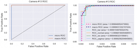
30% of the dataset were used to evaluate the performance of the models created. The performance values obtained using these data vary between 99.51% and 99.85%. Figure 21, Figure 23 and Figure 25 show the heatmaps of each model respectively, while Figure 22, Figure 24 and Figure 26 show the ROC curves of each model respectively.
Camera #4.model
Figure 21. Camera #4.model prediction values heatmap
Figure 22. Camera #4.model ROC curve
In Table 3, the success rates and values obtained for Camera #4 model outputs are given.
Table 3. Camera #4.model results
|
|
Snow(kar) |
Normal |
Fog(sis) |
Rain(Yagmur) |
|
FP |
0 |
0 |
2 |
3 |
|
FN |
2 |
0 |
1 |
2 |
|
TP |
10 |
500 |
146 |
357 |
|
TN |
1006 |
518 |
869 |
656 |
|
TPR |
0.83333333 |
1 |
0.99319728 |
0.99442897 |
|
TNR |
1 |
1 |
0.99770379 |
0.99544765 |
|
PPV |
1 |
1 |
0.98648649 |
0.99166667 |
|
NPV |
0.99801587 |
1 |
0.99885057 |
0.99696049 |
|
FPR |
0 |
0 |
0.00229621 |
0.00455235 |
|
FNR |
0.16666667 |
0 |
0.00680272 |
0.00557103 |
|
FDR |
0 |
0 |
0.01351351 |
0.00833333 |
|
ACC |
0.99803536 |
1 |
0.99705305 |
0.99508841 |
F1score values for Camera #4.model are specified in Table 4. Since the designed model is a multi-class model, the F1weighted value obtained from the averages of the F1 scores of each class is used as the weighted model score.
Table 4. Camera #4.model results
|
|
Score |
|
F1micro |
0.9950884086444007 |
|
F1macro |
0.9729918286611905 |
|
F1weighted |
0.9950075173932358 |
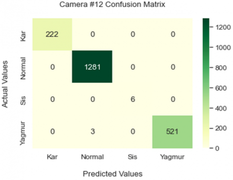
Camera #12.model
Figure 23. Camera #12.model prediction values heatmap
Figure 24. Camera #12.model ROC curve
In Table 5, the success rates and values obtained for Camera #12 model outputs are given.
Table 5. Camera #12.model results
|
|
Snow(kar) |
Normal |
Fog(sis) |
Rain(Yagmur) |
|
FP |
0 |
3 |
0 |
0 |
|
FN |
0 |
0 |
0 |
3 |
|
TP |
222 |
1281 |
6 |
521 |
|
TN |
1811 |
749 |
2027 |
1509 |
|
TPR |
1 |
1 |
1 |
0.99427481 |
|
TNR |
1 |
0.99601064 |
1 |
1 |
|
PPV |
1 |
0.99766355 |
1 |
1 |
|
NPV |
1 |
1 |
1 |
0.99801587 |
|
FPR |
0 |
0.00398936 |
0 |
0 |
|
FNR |
0 |
0 |
0 |
0.00572519 |
|
FDR |
0 |
0.00233645 |
0 |
0 |
|
ACC |
1 |
0.99852435 |
1 |
0.99852435 |
Table 6. Camera #12.model results
|
|
Score |
|
F1micro |
0.9985243482538121 |
|
F1macro |
0.998989898989899 |
|
F1weighted |
0.9985230930476484 |
F1score values for Camera #12 model are specified in Table 6. Since the designed model is a multi-class model, the F1weighted value obtained from the averages of the F1 scores of each class is used as the weighted model score.
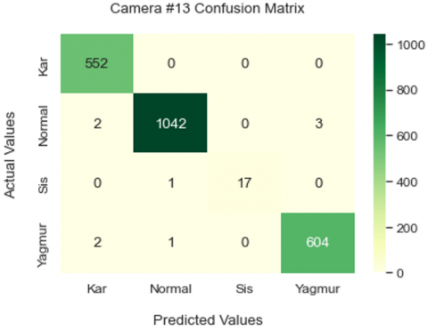
Camera #13.model
Figure 25. Camera #13.model Prediction Values Heatmap
Figure 26. Camera #13.model ROC curve
Table 7. Camera #13.model results
|
|
Snow(kar) |
Normal |
Fog(sis) |
Rain(Yagmur) |
|
FP |
4 |
2 |
0 |
3 |
|
FN |
0 |
5 |
1 |
3 |
|
TP |
552 |
1042 |
17 |
604 |
|
TN |
1668 |
1175 |
2206 |
1614 |
|
TPR |
1 |
0.99522445 |
0.94444444 |
0.99505766 |
|
TNR |
0.99760766 |
0.99830076 |
1 |
0.99814471 |
|
PPV |
0.99280576 |
0.99808429 |
1 |
0.99505766 |
|
NPV |
1 |
0.99576271 |
0.9995469 |
0.99814471 |
|
FPR |
0.00239234 |
0.00169924 |
0 |
0.00185529 |
|
FNR |
0 |
0.00477555 |
0.05555556 |
0.00494234 |
|
FDR |
0.00719424 |
0.00191571 |
0 |
0.00494234 |
|
ACC |
0.99820144 |
0.99685252 |
0.99955036 |
0.99730216 |
The performance rates and values obtained for Camera #13 model outputs are given in Table 7.
F1score values for Camera #13.model are specified in Table 8. Since the designed model is a multi-class model, the F1weighted value obtained from the averages of the F1 scores of each class is used as the weighted model score.
Table 8. Camera #13.model results
|
|
Score |
|
F1micro |
0.9959532374100719 |
|
F1macro |
0.9898821108039307 |
|
F1weighted |
0.995947802599603 |
The hyperparameters used in the training of the models are displayed in Table 9.
Table 9. Hyperparameters of models
|
Total Parameter Size |
5,328,132 |
|
Input Size |
150×150×3 |
|
Optimizer |
adam |
|
Loss Function |
categorical_crossentropy |
|
Epsilon |
1e-07 |
|
Epoch |
100 |
2.3 Image processing
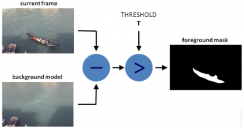
Background Subtraction. Background subtraction is the most commonly used method for detecting moving objects in a fixed camera image is background subtraction. This process takes the difference between the snapshot and the background model. In cases where the difference obtained is more than a predetermined threshold value, objects of the desired size and small pixel groups are separated. The background subtraction process is also explained visually in Figure 27 [39].
Figure 27. Background subtraction
Background subtraction takes place within the cropped ROI area. The background subtraction process and its parameters change dynamically according to the weather model output of the relevant camera. OpenCV modules createBackgroundSubtractorMOG2 [39] and bgsegm.createBackgroundSubtractorMOG [40] are used for background subtraction. Morphological transformations were performed on the black and white image obtained as a result of image processing methods and the detection of moving vehicles in the images was carried out.
In Figure 28 and Figure 29 respectively, there are background extraction, morphological opening/closing operations outputs, and moving object images determined with their borders after these operations using OpenCV [41] in the designed application.
Figure 28. Threshold and morphological closure process
Figure 29. Detected moving object
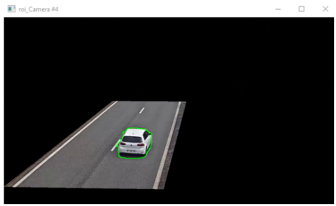
The camera image selected from the camera list was read frame by frame according to the fps value in the broadcast source to detect moving object. Each frame was converted to 1280×720, and then the ROI was cropped according to the ROI boundaries in the config file. The cropped region was added to the main image so that the ROI can be seen in the main image. Figure 30 shows the images obtained.
Figure 30. ROI area and ROI boundaries in main image
2.4 Speed calculation
To calculate speed, the distance is calculated using the Euclidean distance. In the designed system as shown as in Figure 31, the Euclidean distance calculation is performed automatically for the region of interest (ROI) input line coordinates and ROI output line coordinates read from the config file for the 2D plane. The approximate distance equation is given in Eq. (9).
Figure 31. ROI area selection
$d_{\mathrm{aprx}}=d_{e u c} * l(km)$ (9)
The calculated $d_{e u c}$ distance is multiplied by the coefficient $l$ to obtain the approximate $d_{\text {aprx }}$ distance value in $\mathrm{km}$.
In the camera accessed online from France, the lane lines and measurements on the road were used when calculating the distance automatically. For this, the T1 marking method specified in the study [11] was taken as a basis. Here the lane line is 1.5 meters, the lane spacing is 5 meters. For cameras in Istanbul, the system has been calibrated so that the lane line and spacing on the road are 3 meters as according to the guide published by the General Directorate of Highways (KGM) [12].
The difference between the exit time and the entry time and the time spent by the vehicle within the ROI limits can be calculated as given in Eq. (10). Here, $t_{ {ExitTime }}$ represents the moment when the vehicle exits the region of interest, and $t_{{EnterTime }}$ represents the moment when the vehicle enters the region of interest.
$t_{R O I}=t_{ {ExitTime }}-t_{ {EnterTime }}(s n)$ (10)
Speed estimates for each vehicle numbered with different numbers are calculated using $d_{\mathrm{aprx}}$ and $t_{R O I}$ values as given in Eq. (11) [10]. The $k$ value is the speed calibration constant that varies with the camera.
$v_{\mathrm{aprx}}=\frac{d_{\mathrm{aprx}}}{t_{R O I}} * 3.6 * k(\mathrm{~km} / \mathrm{h})$ (11)
2.5 Vehicle detection and tracking
Vehicle tracking was carried out by enumerating and tracking pixel areas larger than the threshold value to be obtained by background extraction from the fixed camera image. Vehicle detection and tracking process is as follows:
If the necessary parameters are provided and the camera is selected, a new video screen opens after the process button is pressed. In Figure 32, the screenshot of the process is given.
Figure 32. Vehicle detected and numbered in ROI area
Entry and exit times to the ROI area for each vehicle number are recorded in real time. Figure 33 shows the visuals of the vehicles entering and exiting the ROI area.
Figure 33. Multiple vehicle detection
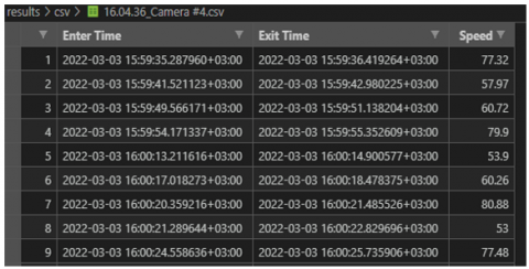
Speed estimates for each vehicle numbered with different numbers are calculated using $d_{\mathrm{aprx}}$ and $t_{\mathrm{ROI}}$ values as given in Eq. (11) [10]. The $\mathrm{k}$ value is the speed calibration constant that varies with the camera. In case the calculated $v_{\text {aprx }}$ value exceeds the speed limit that periodically (e.g., every 15 minutes) updated according to weather predictions, the image of the moment the vehicle exits the ROI is recorded, including the $v_{\text {aprx }}$ value and the vehicle ID. In Figure 34 below, there is an example of csv databases formed as a result of the operation.
Figure 34. Vehicle enter-exit/speed database example
In the application of the speed limit that changes according to the weather, the image taken from any online camera is subjected to two synchronized processes. The CNN weather model is created from the images containing various seasonal conditions obtained from the relevant camera, which is the first process. The success rates of the models created and used in the system are between 99.51% and 99.85%. According to these models, weather forecasts are made at certain periods by using the snapshots taken from the relevant camera. After estimation, hard coded speed limit and image processing parameters are changed automatically.
The second process includes image processing and speed measurements. For this process, firstly, the approximate distance for the camera from the area of interest is calculated. Afterwards, moving vehicle and speed detections are performed using image processing methods. In the system designed, the success rates in vehicle detection, counting and calculation of speed were between 76.46% and 94.67%.
As a result of the process, a csv file is created containing the entry and exit times of each vehicle and the calculated speed values. In case of exceeding the specified speed limits, the snapshot of the relevant vehicle is saved in the specified directory. With this process, vehicle count and vehicle density information can be obtained at certain periods. Figure 35 below shows, as an example, images of vehicles exceeding the speed limit in different weather conditions.
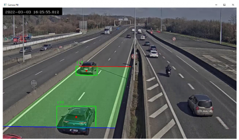
As can be seen in Table 10, the system shows satisfactory performance in vehicle detection. For example, 2256 vehicles were counted at approximately 0.9 vehicles per second during one of the busiest hours of the day in Istanbul with Camera #13. Although the system detected every vehicle in this observation, it showed at least 76.46% success, even with errors caused by incorrectly increasing the vehicle number during the passage of some (long and wide) vehicles or due to lags in the live camera image. As seen in Figure 36, when wide and long vehicles pass through the ROI area, these vehicles can cover the entire area of interest. In this case, the entry and exit time values of the center of the detected object were used when calculating the speed values.
In order to demonstrate the accuracy of the speed estimation, 5 transition were made with the test car on the Camera #13 with normal weather condition and actual speed value was compared with the speed value calculated. As a result of these comparisons, the error rate in speed calculation was found to be 2.54%. The parameters of these transitions and the velocity calculation were verified by estimating with the Kalman filter [13].
Figure 35. Outputs for different weather conditions
Figure 36. Long vehicle detection
Table 10. Results
|
Camera |
Weather |
Predicted Weather |
Process Time |
Total Vehicle Count |
False Vehicle Count |
Vehicle Detection Accuracy |
Average Accuracy |
|
Camera #4 |
Normal |
Normal |
21:05 – 21:47 |
558 |
93 |
%83.33 |
%83.18 |
|
Camera #4 |
Normal |
Normal |
20:10 – 21:03 |
1000 |
94 |
%90.60 |
|
|
Camera #4 |
Normal |
Normal |
21:36 – 22:00 |
113 |
19 |
%83.19 |
|
|
Camera #4 |
Normal |
Normal |
15:28 – 16:57 |
1333 |
181 |
%86.42 |
|
|
Camera #4 |
Rainy |
Rainy |
21:05 – 21.10 |
66 |
15 |
%77.27 |
|
|
Camera #4 |
Rainy |
Rainy |
07:10 – 07:15 |
207 |
45 |
%78.26 |
|
|
Camera #12 |
Normal |
Normal |
19:43 – 19:58 |
450 |
24 |
%94.67 |
%89.55 |
|
Camera #12 |
Rainy |
Rainy |
12:08 – 12.29 |
581 |
35 |
%93.98 |
|
|
Camera #12 |
Rainy |
Rainy |
11:52 – 11.58 |
165 |
33 |
%80.00 |
|
|
Camera #13 |
Normal |
Normal |
12.02 – 12:44 |
2256 |
531 |
%76.46 |
%80.68 |
|
Camera #13 |
Normal |
Normal |
20:21 – 20:27 |
254 |
38 |
%85.04 |
|
|
Camera #13 |
Normal |
Normal |
13:10 – 13:16 |
298 |
63 |
%78.86 |
|
|
Camera #13 |
Normal |
Normal |
13:36 – 13:44 |
400 |
74 |
%81.50 |
|
|
Camera #13 |
Rainy |
Rainy |
13:13 – 13:23 |
196 |
41 |
%79.08 |
|
|
Camera #13 |
Rainy |
Rainy |
13:23 – 13:29 |
243 |
41 |
%83.13 |
3.1 Vehicle speed estimation verification
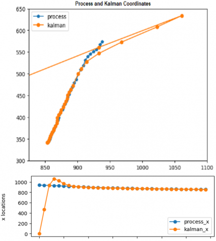
In the designed system, the unit distance difference between the vehicle center points in the previous frame is calculated for each frame. The same calculation was performed for the Kalman filter's center point estimates of the detected vehicle in the next frame in order to verify the velocity estimation. Velocities were calculated for each frame by the ratio of the distance between the obtained two frames to the time differences between the two frames. The Kalman filter starts its estimations from the point (0,0) and continues its estimations according to the vehicle center point in the next frame. After the first few frames, the Kalman filter appeared to make predictions close to the center point.
After the planning, a constant 60 km/h transition was made on the road where Camera #13 live broadcast and weather prediction has made by model. The live video during this transition was recorded without changing the fps value and was used as the video source of the process in the designed application. In this context, speed calculation calibration is provided for the relevant camera. After this calibration, transitions were made again from the relevant cameras and speed estimation was made in the live environment. It has been determined that these estimates are close to the real values and suitable for calibration. In Figure 37, it is seen that the speed value obtained as a result of the process during the transition with the test vehicle is 60.68 km/h.
Figure 37. Speed estimation result with test car (zoomed)
In Figure 38, there is the average velocity value obtained from the Kalman filter estimates at the time of transition with the test car. While the speed value calculated as a result of the process was 60.68 km/h, the average Kalman speed for the same vehicle was 61.74 km/h.
Figure 38. Kalman average speed of test car
Table 11. Relative work comparison
|
Work |
Vehicle Detection & Speed Estimation |
Weather Detection & Classification |
|
Chowdhury et al. [15] |
95.08 - 94.1 |
- |
|
Biswas et al. [16] |
96.55 |
- |
|
Hsieh et al. [17] |
92.8 - 94.8 |
- |
|
Gupte et al. [18] |
90 |
- |
|
Van Pham and Lee [19] |
98* |
- |
|
Bhaskar and Yong [20] |
91.26 |
- |
|
Yaghoobi Ershadi et al. [21] |
94.02 |
- |
|
Tayara et al. [22] |
90.51 |
- |
|
Wicaksono and Setiyono [23] |
87.01 |
- |
|
Chu et al. [24] |
- |
76.6 |
|
Roser and Moosmann [26] |
- |
85.19 |
|
Zhang et al. [25] |
- |
71.39 |
|
Luo et al. [27] |
- |
92.25 |
|
Chen et al. [28] |
- |
75.7 |
|
Our Work |
76.46 - 94.67 |
99.51 – 99.85* |
|
Best performances are in bold and marked “*” |
||
Table 11 shows the results from previous studies and their comparison with our study. As can be seen, our study can make weather prediction more successfully than other studies because it creates a deep learning model with images taken from the camera to be predicted. Since we used image processing methods instead of machine learning for vehicle detection and we perform image processing methods via CPU instead of GPU, our success rate in vehicle detection is slightly lower than other studies.
3.2 Effects of different weather conditions on results
As seen in Table 10, it has been determined that rainy, snowy and foggy weather conditions adversely affect the image processing steps used in vehicle counting and speed calculation. As seen in Figure 39, vehicle and accurate speed detection becomes difficult under heavy rain.
Figure 39. Incorrect vehicle and speed detection under heavy rain (zoomed)
3.3 Effects of camera image features on results
Figure 40. Vehicle detection with low image quality
During the development period, problems such as access problems, physical stabilization of the camera, image quality and closing the viewing angle during rain were encountered. Figure 40 shows that the system designed from any camera with very poor image quality can work for vehicle detection and counting, but the relevant camera images do not have the necessary screen quality for weather detection.
3.4 Effects of image processing parameters on results
If the morphological transformation and background subtraction parameters are not adjusted properly, the surrounding lights cause reflections on the asphalt road, especially in the evening hours. In this case, our image processing algorithm can detect the relevant light movements as cars. In order to prevent this situation, appropriate parameters must be entered for each camera.
In Figure 41, the motorcycle and its silhouette on the rainy ground are not perceived as a vehicle since their volume is small, but are perceived as a part of the other vehicle in the image processing parameter. In this case, the speed calculation of the relevant vehicle will be incorrect. To prevent this, the second value of the structuring element used in the morphological opening process was increased for rainy weather conditions of the relevant camera.
Figure 41. Incorrect image processing parameters result-1
Figure 42. Incorrect image processing parameters result-2 (zoomed)
As seen in Figure 42, if the morphological transformation and background subtraction parameters are not set appropriately, the surrounding lights cause reflections on the asphalt road, especially in the evening hours. In this case, our image processing algorithm can detect the relevant light movements as vehicles. To prevent this situation, appropriate parameters must be entered for each camera.
Figure 43 shows an example of the situation that occurs as a result of improper selection of morphological transformation parameters during the passage of large vehicles. By increasing the initial value of the structuring element used during the morphological closure process, this situation was prevented and a more accurate speed calculation could be obtained after the midpoint of the detected integrated region moved out of the red border line.
Figure 43. Incorrect image processing parameters result-3
Figure 44 shows an example of the error encountered in the number of vehicles and therefore the vehicle speed calculation as a result of numbering the vehicles passing close to each other with the same number, if the minimum value variable used in the tracking algorithm is not entered in accordance with the camera angle and large vehicle passages. This situation was prevented by entering a specific minimum tracking value for each camera.
Figure 44. Incorrect image processing parameters result-4
Public authorities, especially European countries, have developed a will to prevent traffic accidents, possible injuries and deaths by going beyond speed detection and similar traditional approaches in regulating and controlling traffic. There are reports with detailed solutions and targets on this subject. One of the main points highlighted in these reports is to develop systems to dynamically manage traffic with the support of technology.
In this study, it has been shown that electronic monitoring systems can be developed in accordance with the weather. It has been demonstrated that this process can be done without additional cost with deep learning models created from images taken from any camera that can be accessed from the internet. With this study, electronic monitoring deterrence will be increased in reducing the risk of accidents. Therefore, this study shows that weather oriented vehicle speed control can reduce accidents and deaths caused from these accidents.
Vehicle detection, unique numbering of vehicles and estimation of vehicle speed were also performed with this application by using image processing methods. In case of exceeding the speed limit, the snapshots of the relevant vehicles were saved in the specified directory. From the application outputs, the speed estimations that are unique for each vehicle have been verified by two different methods. As the first method, the Kalman filter was used and the average Kalman velocity was compared with the determined velocity estimation. For the second method, transitions from the existing camera at constant speeds were carried out with the test vehicle. The application rate estimates of these transitions are compared with the fixed transition rates.
The fact that the success rates of the weather models, which are the most important part of the system, are in the range of 99.51-99.85%, is the most important basis for the purpose of this study. On the other side, since vehicle and vehicle speed determinations made using snapshot image processing methods over the CPU depend on parameters such as weather, camera angle, camera accessibility, light intensity and angle, it has been seen that vehicle detection and vehicle speed detection success rate is in the range of 76.46-94.67%.
Also with this study can provide the number of vehicles and daily traffic density data can be used in future studies or in transportation plans about the road where the relevant camera will be located. Traffic flow planning, traffic signs and markers planning, road maintenance/repair and development etc. can be planned in the light of these data.
In order to show that the targeted system can be designed without creating additional costs, vehicle detection and speed calculation were performed using image processing methods over the CPU. Thus, it is natural that the success rates obtained in weather detection cannot be achieved in vehicle detection and vehicle speed detection. The momentary frame jumps experienced during the study were the biggest problem in determining the number of vehicles and the speed of the detected vehicle. However, if high-speed GPU containing computers and object detection models are used for vehicle detection, it is predicted that high success rates can be achieved in vehicle detection and vehicle speed detection and the difficulties encountered in section 3.4 can be eliminated.
As a continuation of this study, it is planned to design a new application developed by using object detection models for vehicle and vehicle speed detection.
[1] Hız yönetimi Karar organları ve uygulayıcılar için karayolu güvenliği el kitabı. Emniyet Genel Müdürlüğü Trafik Araştırma Merkezi. http://www.trafik.gov.tr, accessed on Oct. 04, 2023.
[2] OECD/ECMT Transport Research Centre, “SPEED MANAGEMENT,” 2006, https://www.itf-oecd.org/sites/default/files/docs/06speed.pdf, accessed on Oct. 04, 2023.
[3] Turing, A.M. (2009). Computing machinery and intelligence. Springer Netherlands. https://doi.org/10.1093/OSO/9780198250791.003.0017
[4] McCulloch, W.S., Pitts, W. (1943). A logical calculus of the ideas immanent in nervous activity. The Bulletin of Mathematical Biophysics, 5: 115-133. https://doi.org/10.1007/BF02478259/METRICS
[5] Krizhevsky, A., Sutskever, I., Hinton, G.E. (2012). ImageNet classification with deep convolutional neural networks. Part of Advances in Neural Information Processing Systems 25 (NIPS 2012).
[6] “CS 230 - Evrişimli Sinir Ağları El Kitabı.” https://stanford.edu/~shervine/l/tr/teaching/cs-230/cheatsheet-convolutional-neural-networks, accessed on Oct. 04, 2023.
[7] “Introduction to Convolutional Neural Networks | Rubik’s Code.” https://rubikscode.net/2018/02/26/introduction-to-convolutional-neural-networks/, accessed on Oct. 05, 2023.
[8] Yani, M., Budhi Irawan, S.S.M., Casi Setiningsih, S.M. (2019). Application of transfer learning using convolutional neural network method for early detection of terry’s nail. In Journal of Physics: Conference Series, 1201(1): 012052. https://doi.org/10.1088/1742-6596/1201/1/012052
[9] Perihanoğlu, G.M. (2015). Dijital Görüntü İşleme Teknikleri Kullanılarak Görüntülerden Detay Çıkarımı. http://hdl.handle.net/11527/13574.
[10] Chintalacheruvu, N., Muthukumar, V. (2012). Video based vehicle detection and its application in intelligent transportation systems. Journal of Transportation Technologies, 2(04): 305. https://doi.org/10.4236/JTTS.2012.24033
[11] Marc, R., Dominique, G., Evangeline, P. (2012). Generator of road marking textures and associated ground truth applied to the evaluation of road marking detection. In 2012 15th International IEEE Conference on Intelligent Transportation Systems, Anchorage, AK, USA, pp. 933-938. https://doi.org/10.1109/ITSC.2012.6338773
[12] Trafik Güvenliği Dairesi Başkanlığı Trafik Güvenliği İşaretleme Şubesi Müdürlüğü, “Karayolu Trafik İşaretleme Standartları-1”, 2020, Available: https://www.kgm.gov.tr/SiteCollectionDocuments/KGMdocuments/Trafik/IsaretlerElKitabi/KarayoluTrafikIsaretlemeStandartlari1.pdf, accessed on Oct. 04, 2023.
[13] Kalman, R.E. (1960). A new approach to linear filtering and prediction problems. J. Fluids Eng. Trans. ASME, 82(1): 35-45. https://doi.org/10.1115/1.3662552
[14] Saho, K. (2017). Kalman filter for moving object tracking: Performance analysis and filter design. Kalman Filters-Theory for Advanced Applications, 233-252. https://doi.org/10.5772/INTECHOPEN.71731
[15] Chowdhury, P.N., Ray, T.C., Uddin, J. (2018). A vehicle detection technique for traffic management using image processing. In 2018 International Conference on Computer, Communication, Chemical, Material and Electronic Engineering (IC4ME2), Rajshahi, Bangladesh, pp. 1-4. https://doi.org/10.1109/IC4ME2.2018.8465599
[16] Biswas, D., Su, H., Wang, C., Blankenship, J., Stevanovic, A. (2017). An automatic car counting system using OverFeat framework. Sensors, 17(7): 1535. https://doi.org/10.3390/S17071535
[17] Hsieh, J.W., Yu, S.H., Chen, Y.S., Hu, W.F. (2006). Automatic traffic surveillance system for vehicle tracking and classification. IEEE Transactions on Intelligent Transportation Systems, 7(2): 175-187. https://doi.org/10.1109/TITS.2006.874722
[18] Gupte, S., Masoud, O., Martin, R.F.K., Papanikolopoulos, N.P. (2002). Detection and classification of vehicles. IEEE Transactions on Intelligent Transportation Systems, 3(1): 37-47. https://doi.org/10.1109/6979.994794
[19] Van Pham, H., Lee, B.R. (2015). Front-view car detection and counting with occlusion in dense traffic flow. International Journal of Control, Automation and Systems, 13: 1150-1160. https://doi.org/10.1007/S12555-014-0229-7/METRICS
[20] Bhaskar, P.K., Yong, S.P. (2014). Image processing based vehicle detection and tracking method. In 2014 International Conference on Computer and Information Sciences (ICCOINS), Kuala Lumpur, Malaysia, pp. 1-5. https://doi.org/10.1109/ICCOINS.2014.6868357
[21] Yaghoobi Ershadi, N., Menéndez, J.M., Jiménez, D. (2018). Robust vehicle detection in different weather conditions: Using MIPM. PloS One, 13(3): e0191355. https://doi.org/10.1371/JOURNAL.PONE.0191355
[22] Tayara, H., Soo, K.G., Chong, K.T. (2017). Vehicle detection and counting in high-resolution aerial images using convolutional regression neural network. IEEE Access, 6: 2220-2230. https://doi.org/10.1109/ACCESS.2017.2782260
[23] Wicaksono, D.W., Setiyono, B. (2017). Speed estimation on moving vehicle based on digital image processing. (IJCSAM) International Journal of Computing Science and Applied Mathematics, 3(1): 21-26. https://doi.org/10.12962/J24775401.V3I1.2117
[24] Chu, W.T., Zheng, X.Y., Ding, D.S. (2017). Camera as weather sensor: Estimating weather information from single images. Journal of Visual Communication and Image Representation, 46: 233-249. https://doi.org/10.1016/J.JVCIR.2017.04.002
[25] Zhang, Z., Ma, H., Fu, H., Zhang, C. (2016). Scene-free multi-class weather classification on single images. Neurocomputing, 207: 365-373. https://doi.org/10.1016/J.NEUCOM.2016.05.015
[26] Roser, M., Moosmann, F. (2008). Classification of weather situations on single color images. In 2008 IEEE Intelligent Vehicles Symposium, Eindhoven, Netherlands, pp. 798-803. https://doi.org/10.1109/IVS.2008.4621205
[27] Luo, X., Shen, R., Hu, J., Deng, J., Hu, L., Guan, Q. (2017). A deep convolution neural network model for vehicle recognition and face recognition. Procedia Computer Science, 107: 715-720. https://doi.org/10.1016/j.procs.2017.03.153
[28] Chen, L., Ye, F., Ruan, Y., Fan, H., Chen, Q. (2018). An algorithm for highway vehicle detection based on convolutional neural network. Eurasip Journal on Image and Video Processing, 2018: 1-7. https://doi.org/10.1186/s13640-018-0350-2
[29] “Intel® CoreTM i7-9750H Processor.” https://www.intel.com/content/www/us/en/products/sku/191045/intel-core-i79750h-processor-12m-cache-up-to-4-50-ghz/specifications.html, accessed on Oct. 04, 2023.
[30] “Python .” https://www.python.org/, accessed on Oct. 13, 2022.
[31] “PyQt5 Reference Guide — PyQt Documentation v5.15.4.” https://www.riverbankcomputing.com/static/Docs/PyQt5/index.html, accessed on Oct. 04, 2023.
[32] “OpenCV.” https://opencv.org/, accessed on Oct. 13, 2022.
[33] “NumPy.” https://numpy.org/, accessed on Oct. 06, 2023.
[34] “pandas - Python Data Analysis Library.” https://pandas.pydata.org/, accessed on Oct. 06, 2023.
[35] “GitHub - mps-youtube/pafy: Python library to download YouTube content and retrieve metadata.” https://github.com/mps-youtube/pafy, accessed on Oct. 06, 2023.
[36] “TensorFlow.” https://www.tensorflow.org/, accessed on Oct. 06, 2023.
[37] “YouTube.” https://www.youtube.com/, accessed on Oct. 04, 2023.
[38] “İBB Trafik Yoğunluk Haritası.” https://uym.ibb.gov.tr/yharita6/, accessed on Oct. 04, 2023.
[39] “OpenCV: How to Use Background Subtraction Methods.” https://docs.opencv.org/4.x/d1/dc5/tutorial_background_subtraction.html, accessed on Oct. 04, 2023.
[40] “OpenCV: Improved Background-Foreground Segmentation Methods.” https://docs.opencv.org/4.x/d2/d55/group__bgsegm.html, accessed on Oct. 06, 2023.
[41] “OpenCV - Open Computer Vision Library.” https://opencv.org/, accessed on Oct. 04, 2023.