Wenxian Li![]() | Zhimin Liu*
| Zhimin Liu*![]()
© 2023 IIETA. This article is published by IIETA and is licensed under the CC BY 4.0 license (http://creativecommons.org/licenses/by/4.0/).
OPEN ACCESS
In efforts to refine the digital measurement accuracy of steel truss bridge rods, a novel methodology was proposed, integrating laser point cloud technology with advanced image processing. Point cloud data, derived from stationary and handheld scanners, was meticulously fused with image datasets to produce precise rod models. Specialised algorithms tailored for point cloud data segmentation, edge detection, and geometric feature extraction were employed to derive accurate geometric attributes of the rods. Furthermore, deep learning techniques were harnessed for image segmentation and feature extraction, predicting potential deformations and delineating damage areas, significantly enhancing the accuracy of feature recognition. Through finite element analysis, errors introduced from non-fixed deformations during the scanning phase were meticulously rectified. Validations suggest that this innovative digital measurement approach, blending laser point cloud and sophisticated image processing, notably outperforms conventional methodologies in terms of precision and efficiency, offering promising avenues for subsequent research and applications in the realm of digital measurements.
steel truss bridge, 3D scanning technology, point cloud data algorithms, digital measurement, advanced image processing, deep learning, data fusion
In this digital and information-driven era, the expansion and diversification of digital image processing techniques have been observed. These techniques now permeate various sectors, encompassing medical diagnostics, aerospace, industrial inspection, and notably, urban infrastructure maintenance [1-4]. Within this realm, bridges - crucial components of urban transport networks - play an indispensable role. Their structural health is intrinsically linked to traffic safety and efficiency, bearing broader ramifications for life and property safety [5]. Yet, the burgeoning urbanisation process has heralded a proliferation in the quantity and diversity of bridges, thereby intensifying societal scrutiny over their health and safety parameters.
Traditionally, bridge health evaluations were predominantly facilitated through manual surveys. Such approaches, however, have been fraught with numerous pitfalls. It has been noted that manual evaluations are not only time-intensive but also laden with subjectivity, wherein outcomes hinge considerably upon the inspector's proficiency and judgment. Additionally, certain bridge zones, especially those in challenging environments, are deemed inaccessible, further curtailing the thoroughness of these manual assessments. In the face of these limitations, the need for leveraging advanced technological interventions to bolster bridge inspection efficacy and precision became an overarching theme in both academic and engineering arenas.
The emergence of digital image processing methodologies has been perceived as a beacon of hope in this context. Through the acquisition and scrutiny of high-definition bridge images, not only has the inspection process been expeditiously streamlined, but a substantial uplift in the objectivity and fidelity of the outcomes has also been recorded [6]. More so, these innovative techniques have been pivotal in facilitating evaluations of previously inaccessible bridge segments, thus heightening the inspection's comprehensiveness.
However, it is recognised that the domain of digital image processing, despite its prodigious potential, is not without challenges. Paramount concerns, encompassing the enhancement of image resolution, proficient handling of extensive image data, and the refinement of algorithmic accuracy and robustness, are yet to be fully addressed. Given these intricacies, concerted efforts by scholars and practitioners worldwide are ongoing, all in pursuit of uncovering more adept methods for bridge assessment.
Through a meticulous examination of the present landscape and its inherent challenges in bridge evaluation, digital image processing techniques have been identified as potentially transformative agents. Their role in the future of bridge health monitoring and maintenance is anticipated to be pivotal. Their integration is not merely forecasted to augment the efficiency and veracity of bridge assessments, but also to herald significant advancements in bridge health surveillance methodologies. Such advancements are set to be instrumental in fortifying bridge security and enhancing urban vehicular throughput.
Since the twilight of the 20th century, the deployment of digital image processing technology has been extensively witnessed, most notably within the realm of bridge health monitoring. Historically, the evaluation of bridge health was largely contingent on visual inspections or rudimentary mechanical tests [7]. Such methodologies, it was observed, were significantly influenced by the discernment and expertise of engineers and technicians, thereby engendering potential subjectivity and inconsistencies in their findings.
In pursuit of enhanced accuracy and efficiency, endeavours were made to incorporate digital image processing technology into the diagnostics of bridge health. Preliminary studies were characterised by comparisons between bridge images captured over varying temporal intervals, with the primary objective being the discernment of structural alterations and emergent damages [8].
Subsequent technological evolutions catalysed the advent of more nuanced methodologies. Feature extraction from images via advanced image processing technologies emerged as a prominent strategy. Information gleaned from these processed images has been shown to be instrumental in facilitating engineers in the meticulous identification of damage locales, gauging damage severity, and thus, proffering calibrated remediation advisories [9, 10].
In the recent epoch, deep learning and machine learning paradigms have witnessed an ascendancy, and their integration into bridge health diagnostics has been noted. By leveraging these deep learning architectures, it was found that extensive image repositories could be processed autonomously, engendering prompt and precise identification and localisation of structural damages. This modus operandi heralded a paradigm shift in bolstering the efficiency and precision of assessments [11, 12].
However, despite the promising vistas opened by deep learning, challenges in its seamless integration into bridge diagnostics remain rife. Acquiring copious labelled data, imperative for the efficacious training of deep learning models, has been identified as a significant hurdle [13]. Furthermore, issues spanning the assurance of model robustness, adept management of voluminous image repositories, and real-time damage detection in pragmatic scenarios have been areas of fervent academic endeavour [14].
In the backdrop of these antecedent studies and extant technological impediments, a novel bridge health assessment framework, intertwining digital image processing and deep learning algorithms, is delineated in the ensuing study. An adaptive, image-based detection architecture is elucidated, imbued with the capacity to autonomously discern, categorise, and evaluate a spectrum of bridge structural damages. This modality seeks to transcend the constraints of prevailing methodologies and to augment the rigour of bridge health diagnostics. It is posited that this research will unveil novel vistas in bridge health surveillance and provide a sturdy scaffold for subsequent scholarly explorations.
Three-dimensional laser scanning technology, founded upon the principles of laser measurement and reflection, facilitates the generation of point cloud data. This affords timely and precise 3D model representations, pivotal in contemporary architectural and engineering realms [15]. Yet, during practical implementation, it has been observed that the inherent point cloud data can be compromised by environmental interferences and instrumental inaccuracies, necessitating the intervention of advanced image processing techniques for data rectification.
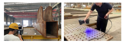
In the context of this investigation, tripod-based scanners, specifically those of FARO and Z+F pedigrees, were employed to assimilate comprehensive point cloud data of steel truss rods. Although these apparatuses boast the capability to rapidly amass a multitude of data points, their inherent fixed incidence angles have been noted to impede the capture of intricate details, such as bolt holes. To circumvent this limitation, additional scans were conducted, leveraging handheld scanner technology [15].
Following data accrual, an array of image processing algorithms was deployed to enhance and distil pivotal data attributes:
• Data Filtering: Noise, inadvertently introduced either by instrumentation or ambient conditions, was mitigated through the application of Gaussian and median filtering techniques.
• Point Cloud Densification: Endeavours were undertaken to procure a more granular model by embracing point cloud interpolation techniques. Through this modality, estimations regarding the position and characteristics of proximate points were formulated, serving to augment point density.
• Feature Extraction: The prowess of deep learning networks, predominantly Convolutional Neural Networks (CNN), was harnessed to autonomously discern and cull salient features, such as bolt holes. Complementary strategies, including edge detection and morphological operations, were additionally employed to accentuate feature visualisation and detection.
• Point Cloud Data Registration: The ICP (Iterative Closest Point) algorithm found application in ensuring harmonious alignment between datasets amassed by both handheld and tripod-based scanning mechanisms, thereby buttressing the coherence and precision of the resultant model.
Figure 1 elucidates the juxtaposition of point cloud data, as garnered on-site through disparate scanning methodologies, with the refined exemplar post the incorporation of sophisticated image processing techniques.
Figure 1. On-site point cloud data: Raw vs. refined
The Point Cloud Library (PCL) is recognised as an open-source algorithm library specifically tailored for point cloud processing operations [16]. The focus of this section is the exploration of methods to extract geometric features from point cloud models via PCL, integrated with state-of-the-art image processing techniques, especially those centred on geometric morphology.
4.1 Geometric feature-based model segmentation and image augmentation
For the appraisal of point cloud data quality, several image enhancement techniques were employed as a preliminary step. Among these were histogram equalisation, sharpening, and noise reduction, which were instrumental in elevating the accuracy of the ensuing operations. Given the intrinsic traits of structural members, plane fitting for rods was undertaken using RANSAC (Random Sample Consensus). Through RANSAC, parameters for a coherent mathematical model were ascertained via a stochastic sampling approach [17]. This procedure not only aided in capturing planar features of the rods but also paved the way for the extraction of geometric features from the identified planes.
In the current study, the deployment of the algorithm comprises two primary phases, both being iteratively executed: To commence, the input data was analysed, from which the minimum required elements were drawn, subsequently dictating the parameters of the mathematical model. Specifically, parameters in the equation x+By+Cz+D=0 were discerned to yield optimum simulation outcomes. Thereafter, elements were categorised based on these parameters. Elements surpassing the set distance threshold were deemed outliers; those within were tagged as inliers. This iterative process persisted until the model with the maximum inliers was selected as the final segmentation. The results of this segmentation were then exported and removed from the point cloud data. Following this, the dataset underwent updates, and the extraction was reiterated until the specified number of planes intended for extraction was achieved.
4.2 Boundary detection and augmentation
Post model plane segmentation, the Alpha Shapes algorithm was employed to delineate the perimeters of each segmented plane [18]. This served to eliminate point cloud data within the plane that lacked geometric feature representation, thereby streamlining the subsequent geometric feature extraction process. Contingent on the model's volume and point cloud density, a parameter α was established. Using α as a radius, a duo of points from the point cloud data was selected to formulate a circle. When α attained a specific magnitude, it did not permeate the interior of the point set, indicating no other point cloud resided within that circle. Instead, it traversed the boundary of that point set, ensuring precise positioning and categorisation, as depicted in Figure 2.
Figure 2. Depiction of the Alpha Shapes algorithm mechanism
4.3 Geometric feature extraction and image segmentation
For the extraction of lines and bolt holes from the model, RANSAC was utilised to facilitate line fitting. The model was formulated as:
$\frac{x-{{x}_{0}}}{m}=\frac{y-{{y}_{0}}}{n}=\frac{z-{{z}_{0}}}{p}$
In this equation, coordinates (x0, y0, z0) represent a point on the spatial line, while m, n, p are indicative of the direction vectors associated with the line.
For the effective extraction of lines, parameters were defined in the following manner:
(1) The objective function was designated as the spatial line fitting model, with an associated distance threshold, aiming to identify the parameter model encompassing the maximum inliers.
(2) The minimum sampling value was determined based on the fewest point clouds present in the extracted line, ensuring the prevention of redundant data.
(3) The condition for ceasing iterations was expressed as:
$m\ge \frac{\ln (1-P)}{\ln \left( 1-{{l}^{N}} \right)}$ (1)
In this condition, p=1-(1-tN)m and t denote the inlier probability. The iteration was designed to guarantee that, under a set confidence level of P (99% in this context), at least one instance of sampling would contain N points from the subset classified as inliers. Here, t is typically perceived as the inlier probability within the entire dataset. As the iteration count augments, the proportion of maximum inliers can exhibit growth. The value for t is chosen in light of the most unfavourable anticipated proportion of inliers.
Subsequent to this step, the region-growing algorithm, a tool of image processing, was incorporated for the extraction of bolt holes. A neighbour search centred on the KD-tree was employed, with particular emphasis on the utilisation of Euclidean clustering [19] for the classification of geometric features in models post edge extraction.
The applications of the KD-tree's nearest neighbour search can be primarily bifurcated into two categories. Initially, a search radius r, centred around point q, was designated to locate points encapsulated by the circle defined by this radius. Following this, a criterion was established for the count of nearest neighbours, K, with the aim to identify the K points in closest proximity to q within the defined circle.
During the clustering procedure, given the stipulated search radius r and the range of nearest neighbour count, the KD-tree nearest neighbour search was applied to the point q within the input dataset Q, yielding the dataset Pi. If the point cloud data within the dataset ceased to grow in number, Pi was then documented as output. The residual point cloud data was subsequently recharacterised as Q for further iterative operations. If not, a new point within Pi was selected as q, and the search method outlined above was reiterated.
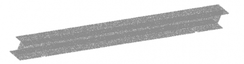
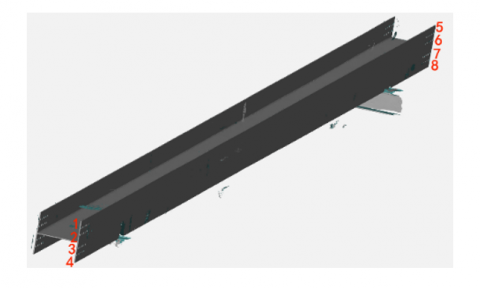
In the undertaken research, a filtering treatment was applied to the point cloud model representing rod members. Conventional image enhancement techniques, such as histogram equalisation and bilateral filtering, were integrated, resulting in a clearer representation of the point cloud data. For the purpose of testing the algorithm, a rod member point cloud model, consisting of a data magnitude in the millions, was selected, as illustrated in Figure 3.
The rod member model used for testing was first subjected to plane segmentation. Here, the spatial equation for the segmented plane was determined. Otsu's method [20], among other classical image segmentation techniques, was incorporated to refine the segmentation outcome. Given the project's stringent precision requirements of up to two decimal places, a distance threshold was set at 0.01mm. The criterion for plane extraction was stipulated to be no less than 0.1 times the quantity of the rod member point cloud. To differentiate between segmented planes, varying colours were employed, as evident in Figure 4, wherein the red portion denotes the unsegmented plane.
Figure 3. Depiction of the point cloud model of bridge members
Figure 4. Depiction of plane segmentation results
Following this, edge detection was executed on the planes extracted. Morphological edge detection [21] was employed to enhance the edges, aiming to ensure a comprehensive extraction of the bolt hole edges while preserving the integrity of the plane. In the determination of the α value, the internal point cloud density was considered, ensuring it remained marginally smaller than the bolt hole radius of the rod member, an approximate of 10-12mm. Subsequent to the extraction of rod member plane edges and bolt hole edges, visual enhancements were carried out, with results captured in Figure 5.
Figure 5. Display of edge extraction results
For the detection of lines on the extracted edges, the Hough Transform [22] was utilised. Adhering to the project's precision standards, a distance threshold of 0.01mm was chosen, with an upper limit set for iteration count at 1000. In this phase, four unique edges of the rod member plane were discerned, each delineated by a distinct colour. The results of this phase were articulated in Figure 6. Linear equations corresponding to these edges were then derived. Incorporating Connected-component analysis from image processing, the extracted plane edges underwent Euclidean clustering [23].
Figure 6. Line extraction results
With a pre-defined search diameter of 25mm, adjustments were made to both the upper and lower bounds of the point cloud clustering. This process culminated in the results presented in Figure 7.
Figure 7. Exhibition of bolt hole extraction results
In the succeeding step, the RANSAC algorithm was employed, supplemented by image fitting techniques, for the spatial circle fitting of the bolt holes that had been extracted. Consistency was maintained with a distance threshold set at 0.01mm and the iteration count capped at 1000.
The synergistic combination of point cloud and image technology was harnessed to present the algorithm's output. Within the predefined precision range, all geometric features were successfully extracted. This extraction of both spatial linear and spatial circle-associated features in the rod member model provided a robust foundation for subsequent geometric feature value computations.
In the process of calculating geometric features of the rod member, methods encompassing traditional three-dimensional spatial geometry were utilised, and integration with image processing techniques was seen, notably in determining geometric attributes such as corner coordinates and bolt hole diameters.
For a more nuanced identification of the rod member's corners, algorithms for edge detection and corner detection, exemplified by the Harris corner detection [24], were employed. Such techniques were instrumental in facilitating key point discernment. From these identified corners, intersections between lines were deduced. By fitting lines adjacent to the segmented plane edge, parameters for each line were outputted, leading to the formulation of the spatial equation for the fitted line. Intersections between the lines were subsequently computed using a specified formula:
$\left\{ \begin{array}{*{35}{l}} \frac{x-{{x}_{1}}}{{{m}_{1}}}=\frac{y-{{y}_{1}}}{{{n}_{1}}}=\frac{z-{{z}_{1}}}{{{p}_{1}}} \\ \frac{x-{{x}_{2}}}{{{m}_{2}}}=\frac{y-{{y}_{2}}}{{{n}_{2}}}=\frac{z-{{z}_{2}}}{{{p}_{2}}} \\\end{array} \right.$ (2)
Upon resolving these equations, corner coordinates (a1, b1, c1) were derived. In a parallel fashion, another set of corner coordinates (a2, b2, c2) was determined. The subsequent step involved utilising the derived distance formula:
$d=\sqrt{{{\left( {{a}_{1}}-{{a}_{2}} \right)}^{2}}+{{\left( {{b}_{1}}-{{b}_{2}} \right)}^{2}}+{{\left( {{c}_{1}}-{{c}_{2}} \right)}^{2}}}$ (3)
From these equations, the length of the rod member, along with the cover plate width and spacing, were ascertained.
In the domain of bolt hole detection, the RANSAC circle fitting was complemented by the integration of circle detection algorithms derived from image processing, notably the Hough Transform for circle detection [25]. Such amalgamations enhanced the precision in determining bolt hole diameters and coordinates of the circle's centre.
The term 'extreme edge hole spacing' is defined as the distance between centres of the bolt holes located at the furthest edges of the rod member. Through the application of image processing techniques, RANSAC and the Hough Transform were engaged to pinpoint two bolt hole centre coordinates, denoted as (x1, y1, z1) and (x2, y2, z2). The formula governing three-dimensional spatial distance was then enacted to gauge the distance between these coordinates, yielding the extreme edge hole spacing for the rod member.
The marriage of image processing techniques with age-old three-dimensional spatial geometry calculations was observed not only to enhance computational accuracy but also to fortify the robustness and stability of the employed algorithms.
In the endeavour to scan rod members and derive their geometric feature values, image processing and computer vision techniques have been regarded as indispensable. Such techniques were leveraged with the intent of attaining a more refined perception of the rod members' geometric structure while also addressing potential anomalies.
7.1 Ascertainment of deformation factors
Deformations in rod members during scanning might have been perceived for myriad reasons. Factors such as self-weight induced deformations, contingent upon the placement of support points, or exogenous influences including temperature variations and exposure to sunlight, could have affected the rod member's surface temperature, consequently leading to deformation.
Such deformation elements were quantified using image processing, which entailed feature detection, edge detection, and evaluating the repercussions of temperature on pixel intensity. Algorithms designed for edge detection, for instance, Sobel or Canny [26], were integrated for delineating the rod member's contours. Meanwhile, feature point matching algorithms, including SIFT or SURF [27, 28], were instrumental in tracking deformations across different temperature gradients.
7.2 Technical procedure of implementation
(1) Before commencing with the three-dimensional laser scanning, the orientation of the rod members was pre-determined through the application of image processing methodologies. Texture analysis coupled with feature detection proved valuable in ascertaining the optimal positioning and sequence of pads. Concurrent with the scanning phase, infrared cameras were utilised to record the rod member's surface temperature. This captured data was then transmuted into relevant temperature data models via image segmentation techniques.
(2) Subsequent to the procurement of point cloud data, image enhancement techniques were deployed for its refinement. This enriched data then became the subject of digital measurements, conducted through the previously mentioned algorithms.
(3) Upon being imported into Abaqus, algorithms such as HOG [29] or those based on Deep Learning methodologies [30], were instrumental in ensuring that the point cloud models were congruent with the intended design blueprints.
(4) Within the realm of Abaqus simulations, the application of computer vision techniques became pivotal for establishing constraint conditions, like identifying support placements using image registration methods.
(5) Deformation simulations, juxtaposed with data from the point cloud model, were analysed using image fusion methodologies. This comparative study facilitated the extraction of accurate measurement outcomes.
(6) The culmination of the measurement process was also enriched with computer vision methodologies. Techniques centred on object detection were pivotal in discerning defects within the rod members, thereby providing insights into the quality of their fabrication.
Through the meticulous implementation of the aforementioned procedures, the geometric feature measurements of rod members were not just elevated in terms of precision, but inherent measurement discrepancies were also aptly addressed.
Image processing techniques played a pivotal role in extracting the geometric features of rod members. The ensuing discussion elucidates their role during application.
8.1 Extraction of rod member geometric features
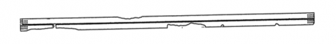
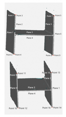
The model under examination and the geometric features requiring extraction are illustrated in Figure 8. Image enhancement techniques [31], such as histogram equalisation and filters, were employed to augment the feature points within the image.
Figure 8. Schematic diagram of extracting geometric features
Planar fitting and segmentation were accomplished using the RANSAC algorithm [31] and edge detection techniques [26]. RANSAC was utilized for estimating planar parameters from point cloud data, whilst edge detection techniques served to identify the boundaries and features of the rod members. The equation for the target plane was given by Ax+By+Cz+D=0, with output coefficients for the spatial plane equation presented in Table 1.
Table 1. Space coefficients of plane equations for member
|
|
A |
B |
C |
D |
|
Plane 1 |
-0.058 |
-1.000 |
0.031 |
9.014 |
|
Plane 2 |
0.061 |
1.000 |
-0.024 |
3.556 |
|
Plane 3 |
0.370 |
-0.016 |
0.929 |
-52.101 |
|
Plane 4 |
0.371 |
-0.011 |
0.929 |
-40.687 |
|
Plane 5 |
-0.056 |
-1.000 |
0.037 |
-484.77 |
|
Plane 6 |
-0.062 |
-1.000 |
0.021 |
-498.89 |
For extracting edges on the segmented plane, the Sobel algorithm [23] and the Canny edge detector [26] were employed. Line fitting was achieved using the Hough transform [25], and the coordinates of each corner point of the rod member were deduced from the intersection points of two adjacent lines, as displayed in Table 2.
Table 2. Coordinate values of each corner point of the member
|
Corner Point Name |
Coordinate Values (x, y, z) |
Corner Point Name |
Coordinate Values (x, y, z) |
|
Point 1 |
-11673.3, 842.548, 4984.7 |
Point 9 |
3264.65, -721.673, -998.71 |
|
Point 2 |
-11846.7, 843.092, 4523.31 |
Point 10 |
3078.36, -723.579, -1457.65 |
|
Point 3 |
-11673.2, 830.034, 4985.89 |
Point 11 |
3267.65, -709.62 -999.59 |
|
Point 4 |
-11858.2, 830.328, 4523.8 |
Point 12 |
3081.23, -710.174, -1459.7 |
|
Point 5 |
-11702.7, 338.788, 4992.18 |
Point 13 |
3298.81, -218.429, -1008 |
|
Point 6 |
-11890.2, 336.914, 4531.91 |
Point 14 |
3113.34, -217.149, -1470 |
|
Point 7 |
-11705.01 350.89 4993.59 |
Point 15 |
3297.68, -230.153, -1008.8 |
|
Point 8 |
-11886.3, 349.999, 4532.69 |
Point 16 |
3114.39, -229.897, -1468.11 |
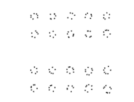
Figure 9. Schematic diagram of bolt hole extraction
For bolt hole extraction, image binarisation techniques [23] and morphological operations [32], such as erosion and dilation, were initially applied to accurately mark the position of the holes. Subsequently, circle detection techniques, specifically the Hough transform-based circle detection [33], were employed to precisely ascertain the bolt hole's position and dimensions. The extraction results for bolt holes on Plane 6 are depicted in Figure 9, with the coordinates of the centre of each bolt hole detailed in Table 3.
Table 3. Coordinate of the centre of each polar hole in Plane 6
|
Bolt Hole |
Coordinate Values (x, y, z) |
|
1 |
-11787, 827.427, 4584.96 |
|
2 |
-11757.3, 827.365, 4658.41 |
|
3 |
-11669.2,827.3,4881.63 |
|
4 |
-11698.2,827.312,4807.95 |
|
5 |
3108.28, -227.228, -1372.03 |
|
6 |
3136.79, -227.273, -1300.81 |
|
7 |
3225.22, -227.299, -1075.14 |
|
8 |
3197.01, -227.378, -1150.83 |
8.2 Calculation of geometric feature values and application of image processing
Once the geometric features of the member have been extracted from the image data, the ensuing pivotal step involves the application of advanced image processing techniques to ascertain the accuracy and consistency of the extracted data.4
Upon the completion of the geometric feature extraction of the inspected member, initially, the extracted coordinate points are subjected to noise filtering. Median filters and Gaussian filters are employed to diminish potential measurement errors and enhance precision. Subsequently, the coordinate distance formula is utilised for the computation of geometric feature values.
To augment the precision of distance calculations, sub-pixel accuracy measurement techniques have been employed. This allows for the acquisition of more precise coordinate positions below the pixel level. According to the measurement criteria in this study:
• The length of the member is determined by calculating the distance between points 2 and 14.
• The width of the cover plate is derived from the distance between points 13 and 14.
• The gap (left) between cover plates is ascertained by the distance between points 12 and 14.
• The gap (right) between cover plates is determined by the distance between points 4 and 8.
• The polar hole spacing is established by measuring the distance between holes 2 and 13.
Table 4. Point cloud measurement values
|
Geometric Feature Dimensions |
Point Cloud Measurements (mm) |
|
Length of the Member |
16150.74 |
|
Width of the Cover Plate |
497.84 |
|
Gap Between Cover Plates (Left) |
481.49 |
|
Gap Between Cover Plates (Right) |
481.23 |
|
Polar Hole Spacing |
16076.04 |
The detailed calculations are presented in Table 4. To further validate the accuracy of these measurements, image registration techniques have been applied to compare the original image with the point cloud model.
8.3 Analysis of simulated deformation of scanned members and application of image processing
8.3.1 Actual engineering measurement conditions and image calibration
During the scanning of the member, it was supported by pads. A pad with a width of 355mm was placed at one end, 1700mm from the end of the member, and another pad with a width of 250mm was placed at the other end, 1980mm from the end.
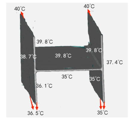
The theoretical measurement temperature of the member is 20℃, while the actual measurement environment was outdoors at 33℃. To compensate for potential errors caused by temperature variations, an infrared thermometer was used to measure the temperature of each plane of the member. At the same time, thermal image processing techniques were applied to analyze the temperature distribution, aiming to optimize measurement accuracy. The distribution of data collection temperatures is shown in Figure 10.
Figure 10. Schematic diagram of scanning temperature for each plane
8.3.2 Analysis of member deformation and benefits of image processing
The constraint between the member and the pads is only the contact surface. During finite element analysis, the pads were simplified as rigid rectangular entities consolidated with the ground. The main focus was on the effects of self-weight and temperature changes on the deformation of the member. To more precisely identify and quantify these deformations, image comparison and analysis techniques were used. By comparing the original and scanned images, the deformation of the member was quantitatively analyzed. The specific finite element analysis results are shown in Figure 11.
Figure 11. Finite element analysis results
In the end, combined with image processing techniques, precise theoretical deformation values at various positions of the member were obtained, as shown in Table 5.
Table 5. Theoretical deformation values
|
Geometric Feature Dimensions |
Theoretical Deformation Values (mm) |
|
Member Length |
-7.53 |
|
Flange Width |
0.22 |
|
Flange Spacing (Left) |
0.21 |
|
Flange Spacing (Right) |
0.22 |
|
Edge Hole Distance |
-4.56 |
8.4 Digital measurement values and error analysis of the member
Image processing techniques have further enhanced the accuracy of point cloud data. Initially, by subtracting the theoretical deformation values from the point cloud measurement values, the final digital measurements of the member were obtained. These were then compared with the actual measurements of the member.
Image registration techniques were used to juxtapose the point cloud measurements with actual measurements to identify and quantify any potential discrepancies. As indicated in Table 6, the differences between point cloud measurements and actual measurements were minimal, verifying the precision of digital measurements. The comparison revealed that digital measurements exhibit high accuracy and precision, underscoring the benefits of this approach.
Table 6. Measurement values and errors of the member
|
Geometric Feature Dimensions |
Theoretical Values (mm) |
Allowable Error (mm) |
Actual Measurements (mm) |
Point Cloud Measurements (mm) |
Error (mm) |
|
Member Length |
16160 |
±5 |
16158 |
16158.27 |
-0.27 |
|
Flange Width |
500 |
±2 |
498 |
498.06 |
-0.06 |
|
Flange Spacing (Left) |
480 |
±2 |
481 |
481.28 |
-0.28 |
|
Flange Spacing (Right) |
480 |
±2 |
481 |
481.01 |
-0.01 |
|
Edge Hole Distance |
16080 |
±1 |
16080.5 |
16080.6 |
-0.10 |
(1) Through the integration of stationary and handheld scanners, a nuanced and precise representation of the member's external appearance and hole clusters was attained. Notably, with the integration of sophisticated image processing methodologies, point cloud data was meticulously fused and analysed. This not only ensured the generation of a high-calibre point cloud model but also augmented scanning efficiency.
(2) Building upon the PCL open-source library foundation and taking into account the unique geometric attributes of steel truss bridge members, a series of algorithmic enhancements and evaluations were undertaken [48]. Through the harnessing of image processing and pattern recognition methods, a pathway for extracting the geometric peculiarities of the member was delineated, leading to the successful digital assessment of the point cloud model anchored in coordinates.
(3) The study ventured into understanding the repercussions of the flexible nature inherent to steel structural members on scanning outcomes, whilst also factoring in practical engineering parameters such as temperature variations and scanning support scenarios. By melding image analytical strategies with finite element analysis tools, theoretical deformation values during the scanning phase were discerned, permitting the rectification of digital measurement outcomes to uphold their veracity.
(4) Within a critical steel truss bridge initiative, the digital measurement methodology elucidated in this research was applied for validation purposes. The derived outcomes not only corroborated the preservation of measurement precision but also underscored the practicality of the proposed technique. This serves as an instrumental reference for future research endeavours focused on bridge-related digital measurement technologies.
Through this research, invaluable insights into the confluence of advanced scanning techniques and image processing methodologies were unveiled, emphasising their pivotal role in enhancing the accuracy and applicability of digital measurement techniques in the realm of bridge engineering.
This paper was supported by the 2021 Natural Science Horizontal Project (Project No.: C21L00650).
[1] Mouhni, N., Elkalay, A., Chakraoui, M., Abdali, A., Ammoumou, A., Amalou, I. (2022). Federated learning for medical imaging: An updated state of the art. Ingénierie des Systèmes d’Information, 27(1): 143-150. https://doi.org/10.18280/isi.270117
[2] Yousif, N.A., Mahdi, G.S., Hashim, A.T. (2022). Medical image encryption based on frequency domain and chaotic map. International Journal of Safety and Security Engineering, 12(4): 467-473. https://doi.org/10.18280/ijsse.120407
[3] El Rejal, A.A., Nagaty, K., Pester, A. (2023). An end-to-end CNN approach for enhancing underwater images using spatial and frequency domain techniques. Acadlore Transactions on AI and Machine Learning, 2(1): 1-12. https://doi.org/10.56578/ataiml020101
[4] Iqbal, S., Khan, T.M., Naqvi, S.S., Holmes, G. (2023). MLR-Net: A multi-layer residual convolutional neural network for leather defect segmentation. Engineering Applications of Artificial Intelligence, 126: 107007. https://doi.org/10.1016/j.engappai.2023.107007
[5] Singh, P., Sadhu, A. (2023). Contact point response-based indirect bridge health monitoring using roboust empirical mode decomposition. Journal of Sound and Vibration, 567: 118064. https://doi.org/10.1016/j.jsv.2023.118064
[6] Zhang, C., Karim, M.M., Qin, R. (2023). A multitask deep learning model for parsing bridge elements and segmenting defect in bridge inspection images. Transportation Research Record, 2677(7): 693-704. https://doi.org/10.1177/03611981231155418
[7] Lang, H., Peng, Y., Zou, Z., Zhu, S., Chen, Z., Zhang, M. (2023). Automated bridgehead settlement detection on the non-staggered-step structures based on settlement point ratio model. Applied Sciences, 13(13): 7888. https://doi.org/10.3390/app13137888
[8] Kruachottikul, P., Cooharojananone, N., Phanomchoeng, G., Chavarnakul, T., Kovitanggoon, K., Trakulwaranont, D., Atchariyachanvanich, K. (2019). Bridge sub structure defect inspection assistance by using deep learning. In 2019 IEEE 10th International Conference on Awareness Science and Technology (iCAST), Morioka, Japan, pp. 1-6. https://doi.org/10.1109/ICAwST.2019.8923507
[9] Trach, R. (2023). A model classifying four classes of defects in reinforced concrete bridge elements using convolutional neural networks. Infrastructures, 8(8): 123. https://doi.org/10.3390/infrastructures8080123
[10] Shashidhar, R., Manjunath, D., Shanmukha, S.M. (2023). CrackSpot: Deep learning for automated detection of structural cracks in concrete infrastructure. Asian Journal of Civil Engineering, 1-12. https://doi.org/10.1007/s42107-023-00754-7
[11] Wang, W., Su, C. (2023). Deep learning-based detection and condition classification of bridge steel bearings. Automation in Construction, 156: 105085. https://doi.org/10.1016/j.autcon.2023.105085
[12] Kumar, D.D., Fang, C., Zheng, Y., Gao, Y. (2023). Semi-supervised transfer learning-based automatic weld defect detection and visual inspection. Engineering Structures, 292: 116580. https://doi.org/10.1016/j.engstruct.2023.116580
[13] Blake, S. (2023). Generating good data for ai-based automatic inspection and remediation of large-scale composite components. International SAMPE Technical Conference.
[14] Sharma, A., Sharma, S., Gulati, S., Choudhury, T. (2022). CAPTCHA robustness-AI approach using to web security. Ingénierie des Systèmes d’Information, 27(2): 303-311. https://doi.org/10.18280/isi.270214
[15] Dong, L., Shuo, Z., Kai, Z., Su, L. C. (2020). A 3D laser scanning method for detecting overall configuration of a pedestrian bridge. Journal of Highway and Transportation Research and Development, 37(9): 57-66.
[16] Liu, Y., Zhong, R. (2014). Buildings and terrain of urban area point cloud segmentation based on PCL. In IOP Conference Series: Earth and Environmental Science, 17(1): 012238. https://doi.org/10.1088/1755-1315/17/1/012238
[17] Zhang, S., Li, S., Zhang, B., Peng, M. (2020). Integration of optimal spatial distributed tie-points in RANSAC-based image registration. European Journal of Remote Sensing, 53(1): 67-80. https://doi.org/10.1080/22797254.2020.1724519
[18] dos Santos, R.C., Galo, M., Carrilho, A.C. (2019). Extraction of building roof boundaries from LiDAR data using an adaptive alpha-shape algorithm. IEEE Geoscience and Remote Sensing Letters, 16(8): 1289-1293. https://doi.org/10.1109/LGRS.2019.2894098
[19] Guo, Z., Liu, H., Shi, H., Li, F., Guo, X., Cheng, B. (2023). KD-tree-based Euclidean clustering for tomographic SAR point cloud extraction and segmentation. IEEE Geoscience and Remote Sensing Letters, 20: 1-5. https://doi.org/10.1109/LGRS.2023.3234406
[20] Otsu, N. (1979). A threshold selection method from gray-level histograms. IEEE Transactions on Systems, Man, and Cybernetics, 9(1): 62-66.
[21] Kraft, M., Kasinski, A. (2008). Morphological edge detection algorithm and its hardware implementation. In Computer Recognition Systems 2, Berlin, Heidelberg: Springer Berlin Heidelberg, pp. 132-139. https://doi.org/10.1007/978-3-540-75175-5_17
[22] Duda, R.O., Hart, P.E. (1972). Use of the Hough transformation to detect lines and curves in pictures. Communications of the ACM, 15(1): 11-15. https://doi.org/10.1145/361237.361242
[23] Gonzalez, R.C., Woods, R.E. (2002). Digital Image Processing (2nd ed.). Prentice Hall.
[24] Harris, C., Stephens, M. (1988). A combined corner and edge detector. In Alvey Vision Conference, Manchester, UK, 15(50): 10-5244.
[25] Hough, P.V. (1962). U.S. Patent No. 3,069,654. Washington, DC: U.S. Patent and Trademark Office.
[26] Canny, J. (1986). A computational approach to edge detection. IEEE Transactions on pattern analysis and machine intelligence, PAMI-8(6): 679-698. https://doi.org/10.1109/TPAMI.1986.4767851
[27] Lowe, D.G. (2004). Distinctive image features from scale-invariant keypoints. International Journal of Computer Vision, 60(2): 91-110. https://doi.org/10.1023/B:VISI.0000029664.99615.94
[28] Bay, H., Tuytelaars, T., Van Gool, L. (2006). Surf: Speeded up robust features. In Computer Vision–ECCV 2006: 9th European Conference on Computer Vision, Graz, Austria, pp. 404-417. https://doi.org/10.1007/11744023
[29] Dalal, N., Triggs, B. (2005). Histograms of oriented gradients for human detection. In 2005 IEEE computer society conference on computer vision and pattern recognition (CVPR'05), San Diego, CA, USA, 1: 886-893. https://doi.org/10.1109/CVPR.2005.177
[30] Krizhevsky, A., Sutskever, I., Hinton, G.E. (2012). Imagenet classification with deep convolutional neural networks. Advances in Neural Information Processing Systems, 1097-1105.
[31] Fischler, M.A., Bolles, R.C. (1981). Random sample consensus: A paradigm for model fitting with applications to image analysis and automated cartography. Communications of the ACM, 24(6): 381-395. https://doi.org/10.1145/358669.358692
[32] Haralick, R.M., Sternberg, S.R., Zhuang, X. (1987). Image analysis using mathematical morphology. IEEE Transactions on Pattern Analysis and Machine Intelligence, PAMI-9(4): 532-550. https://doi.org/10.1109/TPAMI.1987.4767941
[33] Yuen, H.K., Princen, J., Illingworth, J., Kittler, J. (1990). Comparative study of Hough transform methods for circle finding. Image and Vision Computing, 8(1): 71-77. https://doi.org/10.1016/0262-8856(90)90059-E