Hüseyin Firat![]() | Harun Çiğ*
| Harun Çiğ*![]() | Mehmet Tahir Güllüoğlu
| Mehmet Tahir Güllüoğlu![]() | Mehmet Emin Asker
| Mehmet Emin Asker![]() | Davut Hanbay
| Davut Hanbay![]()
© 2023 IIETA. This article is published by IIETA and is licensed under the CC BY 4.0 license (http://creativecommons.org/licenses/by/4.0/).
OPEN ACCESS
Hyperspectral remote sensing images (HRSI) comprise three-dimensional image cubes, containing a single spectral dimension alongside two spatial dimensions. HRSI are presently among the foremost essential datasets for Earth observation. The task of HRSI classification is intricate due to the influence of spectral mixing, leading to notable variability within classes and resemblances across classes. Consequently, the field of HRSI classification has garnered significant research attention in recent times. Convolutional Neural Networks (CNNs) are harnessed to address these issues, enabling both feature extraction and classification. This study introduces a novel approach for HRSI classification called the hybrid 3D-2D depthwise separable convolution network (Hybrid DSCNet), which leverages multiscale feature integration. Within the Hybrid DSCNet, diverse kernel sizes contribute to an enriched feature extraction process from HRSI. The conventional 3D-2D CNN, while effective, comes with a computational load. Instead of using the standard 3D-2D CNN, this study adopts the 3D-2D DSC architecture. This approach partitions the conventional convolution into two components: pointwise and depthwise convolution, yielding a substantial reduction in trainable parameters and computational complexity. To evaluate the proposed method, the Indian Pines dataset along with WHU-Hi subdatasets (LongKou-LK, HanChuan-HC, and HongHu-HH) were employed. Employing a 5% training sample, impressive overall accuracy scores were achieved: 94.51%, 99.78%, 97.06%, and 97.27% for Indian Pines, WHU-LK, WHU-HC, and WHU-HH, respectively. Comparative analysis of the proposed approach with cutting-edge techniques within the literature reveals its superior performance across the four HRSI datasets. Notably, the Hybrid DSCNet attains enhanced classification accuracy while maintaining lower computational overhead.
depthwise separable convolution (DSC), convolutional neural network (CNN), hyperspectral image classification, remote sensing, hybrid CNN
Hyperspectral remote sensing images (HRSI) are represented as 3D (one spectral-two spatial) hypercubes. These images consist of hundreds of spectral bands compared to RGB and multispectral images [1]. Moreover, they encompass abundant spectral characteristic data. This wealth of spectral feature information enhances the precision of identifying and categorizing terrestrial objects [2]. Thus, it is frequently used in applications such as astronomy, agriculture, military surveillance, land fire monitoring and cover analysis, crop monitoring [3-7].
The abundant spectral feature information of the original HRSI causes spectral redundancy. This reduces the HRSI classification (HRSIC) performance. To address this challenge, techniques for reducing dimensionality are applied to the initial HRSI data. Methods like Linear Discriminant Analysis (LDA), Incremental Principal Component Analysis (IPCA), Independent Component Analysis (ICA), Principal Component Analysis (PCA), Locally Linear Embedding (LLE) and Kernel PCA are employed for this purpose [8-10]. The most commonly used method among these DRMs is PCA. PCA is an unsupervised and linear DRM. It can remove large amounts of excess spectral information from HRSI data while preserving the spectral information of the principal components (PCs) with a larger contribution of variance. After PCA, the number of spectral dimensions decreases and the computational cost reduces [11].
Due to the importance and complexity of classification in HRSI, HRSIC has attracted significant research attention. Traditional HRSIC methods such as support vector machine (SVM) [12], logistic regression [13] and k-nearest-neighbors (KNN) [14] usually rely on using many spectral features information for HRSIC. Nevertheless, due to the presence of both spectral band redundancy and strong inter-band correlations within HRSIs, these traditional classifiers often exhibit inadequate performance. In addition, these traditional HRSIC classifiers, which use only spectral features, cannot acquire important spatial information, thus reducing their classification accuracy. The most straightforward approach to enhance classification outcomes involves the creation of classification techniques that jointly utilize spatial-spectral characteristics. Spatial features are combined with spectral features in HRSIC using methods such as morphological profiles [15], multiple kernel learning [16], superpixel [17] and sparse representation [18]. The use of spectral feature information together with spatial feature information increases the classification performance. Nonetheless, the majority of conventional classifiers for HRSIC tend to manually extract features that combine spatial and spectral features.
Over the past few years, approaches founded on deep learning (DL), particularly Convolutional Neural Networks (CNNs), have emerged and gained extensive application within the realm of HRSIC [3]. Unlike traditional HRSIC methods, features are extracted automatically with deep learning-based methods. These features are then used in classification [19]. Because CNN provides more distinctive features in HRSIC, it has pretty good feature learning. In order to analyze classification problems more easily, the learned features should be distinctive [20]. This significantly increases classification performance. Because of this rationale, techniques that rely on CNNs are considered some of the most robust methodologies applied in HRSIC for the extraction of more intricate spatial-spectral features. These methods are widely used in studies by most researchers as they increase the accuracy of HRSIC.
Roy et al. [1] formulated an efficient S3EResBoF (spectral–spatial squeeze and excitation residual bag-of-feature) learning approach tailored for HRSIC. S3EResBoF integrates residual learning blocks for both spatial and spectral enhancement, thus elevating the classification performance. Furthermore, a squeeze and excitation (SE) network succeeds each residual block. The S3EResBoF methodology's efficacy was assessed using the Pavia University (PU), Salinas (SA) and Indian Pines (IP) datasets. In the case of IP, 30 PCs were selected through PCA, while for SA and PU, 15 PCs each were chosen. The method's applications involved a 10-20% training sample ratio and a 15×15 window dimension. The achieved Overall Accuracy (OA) values at different training sample sizes for SA, PU, and IP were as follows: at 20% training sample, 100%, 99.97%, 99.87% for SA, PU, and IP respectively; and at 10% training sample, 99.49%, 99.77%, 99.98%, respectively. Cao and Guo [5] propose an innovative HRSIC network that combines 3D and 2D aspects. This network leverages hybrid dilated convolution to construct high-dimensional residual networks, facilitating the extraction of spectral as well as spatial features. Applications were made on IP, Kennedy space center (KSC) and PU without using any DRM. The OA values in the applications using 7×7 window size, 20% for IP and KSC,10% for PU training sample were obtained as 99.89% for KSC, 99.81% for PU and 99.46% for IP. Roy et al. [21] introduced the A2S2K-ResNet (Attention-based adaptive spectral–spatial kernel ResNet) technique tailored for HRSIC. A2S2K-ResNet adopts 3D convolutional kernels that blend spatial and spectral attributes, and these kernels automatically adjust their receptive field dimensions through end-to-end training. From the chosen 3D kernel feature maps, spatial-spectral features are typically extracted using specially crafted Residual Blocks. Notably, each Residual Block is succeeded by an efficient mechanism for feature recalibration, a step aimed at augmenting the discriminative potency of convolutional feature maps. Applications were made using KSC, IP and PU datasets without using any DRM. The OA values in the applications using 9×9 window size and 10% training sample were obtained as 99.34% for KSC, 99.85% for PU, and 98.66% for IP. Roy et al. [22] formulated the HybridSN (Hybrid SpectralNet) technique for HRSIC, which seamlessly integrates both 2D and 3D CNN components. Within this approach, 2D CNN is employed for capturing spatial features, while 3D CNN is utilized for extracting spectral-spatial characteristics. The method's efficacy was evaluated through applications conducted on the IP, SA, and PU datasets. Using PCA, PCs were selected 30 for IP, and 15 for SA and PU. The applications encompassed a window size of 25×25 and a 30% training sample. Employing HybridSN yielded impressive OA results: 100%, 99.75%, and 99.98% for SA, IP, and PU, respectively. In Ahmad's study [23], a novel approach named FC3D CNN was developed to enhance classification accuracy, relying solely on 3D CNN. Furthermore, the IPCA technique was employed to diminish spectral band redundancy. Through IPCA, the count of spectral bands was reduced to 20, a value that was also adopted for the applications. Testing on the SA, IP, and PU datasets, with a training sample size of 10% and a window size of 11×11, yielded OA outcomes of 98.06%, 97.75%, and 98.40%, respectively. Roy et al. [24] devised the FuseNet technique, featuring a bilinear fusion mechanism applied to distinct squeeze variants like maximum and global pooling. In the FuseNet approach, the merged squeeze and excitation network is integrated with a residual block. During the applications, PCA was employed with 30 PCs for IP and 15 PCs for both SA and PU. Utilizing a 20% training sample and a window size of 15×15, the achieved OA figures were 99.01%, 99.42%, and 99.68% for PU, SA, and IP, respectively. Iyer et al. [25] introduced an approach for HRSCI that leverages Inception modules. Subsequently, they incorporated both Inception Residual Network and HybridSN components into their developed Inception module. The applications, conducted with a window size of 25×25, a training sample size of 30%, and using 30 PCs for IP and 15 PCs for both SA and PU, yielded impressive OA outcomes: 100%, 100%, and 99.76% for PU, SA, and IP, respectively. Xu et al. [26] enhanced the Multiple Spectral Resolution 3D CNN for HRSIC by integrating several elements: the multiple spectral resolution module, spectral dilated convolutions, 3D convolution, and residual connections. As a preprocessing step, PCA is applied to the HRSI data, followed by applications with 100 PCs representing spectral bands. The evaluations were conducted on the Botswana (B), SA, PU, and IP datasets using a 10% training sample and a window size of 9x9. The achieved OA values for these applications were 98.80%, 99.96%, 99.62%, and 98.10%, respectively. Gao et al. [27] devised an innovative multi-scale ResNet strategy intended for HRSIC. This multi-scale ResNet framework integrates DSC as the initial step. Subsequently, the conventional DC within the DSC is substituted with mixed DC, amalgamating diverse kernel sizes. Lastly, this mixed DC is incorporated into the residual block, yielding a multiscale residual block. The method's efficacy was assessed through applications employing the SA, Pavia Center, and PU datasets. During training, 20 random samples were drawn from each class within the datasets. Applying PCA, 15, 10, and 10 PCs were selected for SA, PU, and Pavia Center, respectively, followed by conducting the applications. The window size was set at 15×15 for both PU and SA, and 9×9 for Pavia Center. As a result of these applications, the obtained OA figures were 98.69%, 96.50%, and 96.84% for Pavia Center, PU, and SA, respectively. Fırat et al. [28] enhanced a hybrid approach aimed at HRSIC, which fuses the potential of 3D CNN and the 2D DSC process. Within their proposed framework, evaluations were executed employing 30, 15, and 15 PCs for IP, PU, and SA, respectively, following a PCA preprocessing step. A window size of 11×11 and training samples accounting for 20%, 10%, and 10% were employed for IP, PU, and SA, respectively. Through these applications across the three datasets, the attained OA values stood at 99.90% for SA, 99.83% for PU, and 99.32% for IP. Zheng et al. [29] introduced a hybrid CNN approach, enhanced with covariance pooling, for HRSIC. The method's initial stage entails 3D CNN for the extraction of both spectral and overall features, which is followed by 2D CNN for spatial feature extraction. Furthermore, the method leverages the covariance pooling technique to precisely capture quadratic details from spatial-spectral feature maps. Employing a window size of 25×25 and a 30% training sample, the applications conducted on the PU, SA, and IP datasets yielded impressive OA figures: 99.85% for PU, 100% for SA, and 99.58% for IP. Sun et al. [30] improved a spatial-spectral attention network (SSAN) for HRSIC. SSAN method primarily consists of spatial and spectral modules consisting of simple 3D CNN layers. Then, the attention module was added to specific locations of the spatial spectral modules to extract more distinctive features of the HRSI hypercubes. In performed applications with IP, PU and SA without any preprocessing, OA values of 95.49%, 98.02% and 96.81% were acquired, respectively. Gong [31] devised an approach featuring a multi-scale SE pyramid pooling network. This method comprises components such as a SE block, a multi-scale 3D CNN, and pyramid pooling modules incorporating 2D CNN. By applying this technique to the PU, SA, and IP datasets, with training samples of 0.5%, 0.5%, and 5%, respectively, the achieved OA values stood at 96.56% for PU, 97% for SA, and 96.09% for IP. Additionally, when the proposed method was employed on the high spatial resolution WHU-LK dataset with a 0.1% training sample, an OA value of 97.31% was obtained. Ge et al. [32] enhanced a profound network architecture centered on multi-branch feature integration for the task of HRSI classification. The proposed hybrid strategy combines both 2D CNN and 3D CNN, employing varying kernel sizes across distinct branches. Additionally, in contrast to the ReLU activation function, which has been commonplace in prior studies, the Mish function was adopted. When applied to the IP, SA, PU, and B datasets with a training sample size of 5%, the classification accuracy was determined to be 96.07% for IP, 99.94% for SA, 99.52% for PU, and 96.44% for B. Yang [33] introduced an innovative CNN known as Synergistic Convolutional Neural Network (SyCNN) for the purpose of HRSIC. SyCNN encompasses a blend of both 3D-2D CNN and data interaction modules, facilitating the fusion of spatial-spectral feature insights. Additionally, a 3D attention mechanism is presented, which effectively filters out any interfering information and features prior to reaching the fully connected layer. Employing a randomized 30% training sample, the attained classification accuracy values for the IP, KSC, and B datasets were 97.31%, 98.92%, and 99.79%, respectively. Taking into account the existing research in this domain, it becomes evident that there remains a requirement for the advancement of DL-driven approaches aimed at enhancing the precision of HRSIC. This serves as the impetus behind our undertaking.
CNN offers a superior classification accuracy while extracting insights from spatial-spectral feature information. In this context, it has demonstrated its significance as a prevalent technique in the realm of HRSIC compared to alternative DL approaches. However, the CNN approach does have its drawbacks. For instance, during the gradient descent procedure, it's prone to converging to local minima, and the pooling layer often leads to a loss of valuable information. In HRSIC, it's imperative to consider not only spatial features but also spectral features. Over the past years, CNN has been widely employed in HRSIC to extract spatial features, spectral features, and even spectral-spatial features in tandem. Utilizing 2D CNN, researchers can capture spatial features while struggling to acquire spectral information. Given that HRSI possesses a three-dimensional structure, its spectral attributes hold great importance. Employing 3D CNN enables the extraction of spectral-spatial features, albeit at the expense of increased computational demands. Furthermore, relying solely on 3D CNN can potentially lead to reduced classification accuracy, particularly when distinct classes in HRSIs exhibit similar textures across numerous spectral bands. To mitigate these challenges, hybrid CNN methodologies, which blend the application of 2D and 3D CNN, offer a solution. The integration of hybrid CNN methodologies effectively leverages both spatial and spectral feature insights, yielding a beneficial impact on the classification performance. Additionally, the incorporation of 3D and 2D CNN approaches, each employing distinct kernel sizes, facilitates the amalgamation of diverse features. Furthermore, the adoption of a multi-scale network architecture imparts a heightened enrichment to the feature extraction process from HRSI. In this scenario, the potent feature extraction capacity exhibited by the combined 3D-2D CNN, complemented by multi-path feature fusion, endows the network with the ability to operate effectively even with a limited amount of training data. These considerations underscore our rationale for introducing a hybrid 3D-2D CNN model that hinges on multi-path feature fusion to enhance HRSIC. An additional driving force for the proposed multi-path hybrid methodology is the integration of 3D-2D DSC alongside 3D and 2D CNN blocks. The inclusion of 3D DSC and 2D DSC blocks is strategically aimed at reinforcing the classification robustness and maximizing accuracy within the proposed hybrid framework. The contributions of the method introduced in this study are outlined as follows:
1. We've introduced a hybrid CNN approach that hinges on the fusion of multiscale features to enhance HRSIC. Within this proposed methodology, we amalgamate features that are derived from diverse kernel sizes, thus facilitating the incorporation of more comprehensive feature insights from HRSI. Moreover, the adoption of a multiscale network architecture serves the central objective of augmenting the richness of extracted features from HRSIs.
2. Within the existing body of literature, the prevailing approach for HRSIC typically involves the utilization of 2D DSC. However, it's important to note that, akin to the functioning of 2D CNN, 2D DSC is primarily geared towards the extraction of spatial features. Given that our HRSI data is inherently three-dimensional and spectral attributes carry significant weight, we have opted to integrate 3D DSC in conjunction with 3D CNN. This amalgamation enables the extraction of spatial-spectral feature insights from the data. It's true that the application of standard 3D convolution incurs an elevated computational cost. Nonetheless, the introduction of 3D DSC serves to bifurcate the conventional convolution process into two distinct operations: DC and PC. This deliberate segmentation results in a substantial reduction of the total number of trainable parameters and subsequently curbs computational expenses. An additional motive underpinning this study is the pursuit of diminished trainable parameters alongside improved classification outcomes. To address this aim, we have adopted the approach of incorporating both 3D DSC and 2D DSC. This strategic inclusion serves a dual purpose of minimizing the number of trainable parameters while concurrently enhancing the quality of classification results.
3. By the incorporation of 2D and 3D DSC layers into the framework of the Hybrid CNN approach, we proceeded to evaluate the resultant classification outcomes across various datasets, namely IP, WHU (LK, HC and HH). This examination yielded OA measurements of 94.51%, 99.78%, 97.06%, and 97.27% for the respective datasets of IP, WHU-LK, WHU-HC, and WHU-HH. An analysis of these accuracy values reveals that the inclusion of both 3D and 2D DSC layers leads to improved outcomes while also entailing a reduction in the number of trainable parameters.
The subsequent sections of this study are organized as follows: Section 2 introduces the proposed multiscale Hybrid DSCNet and the theoretical foundation of the Hybrid DSCNet, comprising the 3D/2D CNN and 3D/2D DSCNet. The same section also encompasses details about the employed datasets. Section 3 is dedicated to the presentation of applications pertaining to the datasets, along with the corresponding classification outcomes. An overall evaluation of this paper is provided in Section 4.
2.1 3D/2D Convolutional neural networks (CNN)
2.1.1 2D CNN
CNN designs, a type of DL methods, find common application in research for tasks such as categorizing images and identifying and localizing objects. The CNN architecture draws inspiration from ANNs and possesses the capability to acquire comprehensive information seamlessly. Moreover, CNN represents a DL strategy wherein ANNs encompass a forward processing and a FE layer, in contrast to conventional neural networks. The CNN comprises two primary layer. One of these layer corresponds to the convolutional layer, while the other pertains to the pooling layer. CNNs aspire to capture pivotal attributes of the image via fundamental operations executed across these dual layers.
(1) Convolutional layer
The foundation of DNNs is established by the convolutional layer. This layer relies on the movement of compact filters like 2×2, 3×3, and 5×5 across the entirety of the image. As a result, a novel image is generated through the extraction of finer details within the image.
(2) Pooling layer
The pooling layer constitutes a technique utilized to reduce dimensionality within DL methods. In general, actions aimed at dimension reduction result in the potential loss of information and subsequent performance decline. Nevertheless, pooling offers benefits such as preventing model overfitting and inducing lower computational burden. This procedure is executed using specific classes of filters, similar to the convolutional process. These filters traverse the image, and pooling is executed by selecting either the highest or average values from the pixels within the image. Maximum pooling involves the determination of the most significant value among the pixel values contained within the filter's spatial extent. Average pooling operates on the principle that the summation of pixel values encompassed by the filter area is divided by the dimensions of the filter window.
(3) Activation layer
Within CNNs, a crucial procedure involves the integration of the activation function. ReLU stands as the prevailing choice for activation functions in methods constructed upon DNNs. As demonstrated in Eq. (1), a pivotal attribute of this layer is its ability to nullify negative values within the input data. This approach accelerates network learning through the utilization of the ReLU function.
$ReLU(t)=\left\{\begin{array}{l}0 & if\,\,\, t<0 \\ t & if \,\,\, t \geq 0\end{array}\right.$ (1)
(4) Normalization layer
The Normalization layer is employed to standardize the data derived from layers constructed using CNNs. This procedure ensures that the input data conforms to a specific range, leading to a beneficial impact on network performance.
(5) Fully connected (FC) layer
The FC layer constitutes a unidimensional matrix that establishes connections with all neurons within the preceding layer. Typically positioned towards the conclusion of the CNN structure, these layers serves to enhance class scores. Furthermore, the count of these layers can differ within DL-based methods.
(6) Dropout layer
Within CNNs, the Dropout layer serves to avert overfitting in FC layer or the network's excessive retention of data. This layer operates by excluding specific nodes via defined threshold values. In this manner, the network's efficacy is enhanced by discarding superfluous and less influential data.
(7) Classification layer
The final layer in the CNN method is the classification layer, where the classification operation takes place. The output values of this layer correspond to the quantity of classes, which is determined by the count of objects for recognition. Within DL methods, the softmax classifier is extensively applied within this layer. The softmax classifier produces probabilities ranging from 0 to 1 for every class. Consequently, the class predicted by the method corresponds to the class associated with the highest probability value [34, 35].
For given x inputs, the outcome of an individual neuron is depicted as presented in Eq. (2).
$t=f(w * x+b i a s)$ (2)
Within Eq. (2), f(.) denotes a non-linear activation function that is employed on a summation of weighted inputs. The weight w signifies the filter weight. In the context of 2D CNN, convolution is conducted with a 2D filter, representing the conventional convolution operation. When this typical 2D CNN is employed on HRSI data, solely spatial FE are obtained. The expression for the extraction of spatial features through the use of a 2D CNN is demonstrated in Eq. (3).
$t_{m n}=f\left(\sum_l \sum_{i=0}^{h-1} \sum_{j=0}^{w-1} k_{i j} x_{(i+m)(j+n)}+ bias_{m n}\right)$ (3)
As indicated by Eq. (3), k refers to the 2D convolutional kernel with dimensions h×w. The feature tmn is derived from the position (m,n). For a 2D image scenario, the process of 2D convolution is executed across all feature maps (l) within the recipient region, aggregating all values to apply nonlinear activation.
2.1.2 3D CNN
Given that HRSI data exists in a 3D format, the application of a 2D CNN fails to yield spectral feature insights. In such instances, a 3D CNN featuring 3D convolutional strata becomes essential. Through the utilization of a 3D CNN, the amalgamation of spatial-spectral features occurs. The expression utilized to extract features using a 3D CNN is illustrated in Eq. (4).
$t_{m n d}=f\left(\sum_l \sum_{i=0}^{h-1} \sum_{j=0}^{w-1} \sum_{r=0}^{b-1} k_{i j r} x_{(i+m)(j+n)(r+d)}+bias_{m n d}\right)$ (4)
According to Eq. (4), b denotes the extent of the 3D filter along the spectral dimension. The feature tmnd is derived from the position (m,n,d). The kernel (k) is designed in a 3D manner, enabling feature extraction through the application of 3D convolution to HRSI data. Traditional 2D CNNs solely employ convolution to generate 2D feature maps on spatial dimensions, encompassing all prior-layer feature maps. However, for 3D HRSIC, the acquisition of spatial-spectral features holds great importance. The drawback of utilizing a 2D CNN lies in its inability to extract spectral features. While 3D CNNs extract spatial-spectral features, they introduce increased computational complexity. This heightened complexity is perceived as a downside of adopting 3D CNNs. To address these challenges, the utilization of hybrid CNN methods has become prevalent.
2.2 3D/2D DSCNet
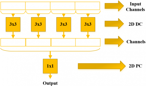
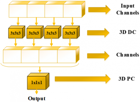
Within the developed multiscale technique, diverse attributes are acquired through the execution of multiple convolutional operations. Nevertheless, employing a multitude of convolutional kernels leads to an upsurge in the count of trainable parameters. DSC offers a viable strategy for curtailing the number of trainable parameters. DSC performs convolutional processing in two distinct stages. Firstly, Depthwise Convolution (DC) is executed, followed by Pointwise Convolution (PC). The PC is essentially a typical 1×1 convolution. Unlike conventional convolution, DSC dissects the process into two stages: DC autonomously filters each input channel, and subsequently, PC amalgamates the DC outputs by means of a 1×1 convolution. In this regard, DSC can also be characterized as a factorized convolution approach [36-38]. Illustrated in Figure 1a, the utilization of DSC in a 2D context involves executing convolutional procedures separately for each channel of the input image via DC, thereby enabling the extraction of spatial attributes in individual dimensions. Subsequently, PC with a 1×1 kernel is employed on the feature maps generated through DC. This PC amalgamates feature maps across channels. Given that HRSI is three-dimensional, the simultaneous capture of spatial-spectral characteristics is imperative. In such instances, 3D convolution procedures are enacted. However, the computational complexity associated with 3D convolution remains substantial. The objective is to mitigate this computational load by implementing 3D DSC. Thus, the concept of DSC naturally extends to 3D convolutions. This entails a straightforward transition by substituting 2D convolutions in 2D DSC with corresponding 3D operations. As depicted in Figure 1b, 3D DSC can be disassembled into two stages: DC and PC. While 3×3 DC and 1×1 PC are applied in the context of 2D DSC, 3D DSC integrates 3×3×3 DC and 1×1×1 PC layers.
The 3D conventional convolution and 3D DSC computational costs are as follows: The way to perform a convolution operation on a 3D feature matrix of (l,w,h,c) is to use a filter with size (k×k×k) to go over the 3D matrix. l,w,h,c indicate the length, width, height and channels, respectively, while k denotes side length of the filter. When a standard 3D convolution operation is applied to an input feature matrix (F) of size $l_F \times w_F \times h_F \times c_F$, a feature output matrix (G) of size $l_G \times w_G \times h_G \times c_G$ is obtained. $c_F$ and $c_G$ indicate the number of channels before and after 3D convolution. The 3D convolution kernel (K) will be $k \times k \times k \times c_F \times c_G$. As a result of the standard 3D convolution process, the computational cost will be as in Eq. (5).
$cost_{standart\_conv}=k \times k \times k \times c_F \times c_G \times l_F \times w_F \times h_F$ (5)
The 3D DSC operation consists of two stages, namely, 3D DC and 3D PC (or 1×1×1 convolution). With DC, a 3×3×3 kernel size convolution process is applied to each channel separately. As a result of this process, the computation cost is as in Eq. (6).
$cost_{DC}=k \times k \times k \times c_F \times l_F \times w_F \times h_F$ (6)
(a)
(b)
Figure 1. (a) 2D DSC, (b) 3D DSC
In order to bring together the separate channels and to ensure adequate information exchange between the channels, it is necessary to join these channels into a single new feature map. This operation is performed with PC. That is, the 1×1×1 filter is used to apply a linear combination to the feature maps acquired as a result of the output of the DC. The computational cost of the PC is as in Eq. (7).
$cost_{P C}=c_G \times c_F \times l_F \times w_F \times h_F$ (7)
The total computational cost obtained by combining DC and PC is as in Eq. (8).
${cost}_{D C}+{cost}_{P C}=k \times k \times k \times c_F \times l_F \times w_F \times h_F+c_G \times c_F \times l_F \times w_F \times h_F$ (8)
When comparing 3D DSC with standard 3D convolution, the result is obtained as in Eq. (9).
$\frac{{cost}_{D C}+{cost}_{P C}}{cost_{standart\_{conv}}}=\frac{k \times k \times k \times c_F \times l_F \times w_F \times h_F+c_G \times c_F \times l_F \times w_F \times h_F}{k \times k \times k \times c_F \times c_G \times l_F \times w_F \times h_F}=\frac{k \times k \times k \times c_F+c_G \times c_F}{k \times k \times k \times c_F \times c_G}=\frac{1}{c_G}+\frac{1}{k^3}\approx\frac{1}{k^3}$ (9)
$c_G$ channel size is big number (usually 32, 64, 128, 256, etc.). This makes $\frac{1}{c_G}$ very small. $\frac{1}{k^3}$ is depending on the side length of kernel. Even when the kernel is small and of side length 2, $\frac{1}{k^3}$ is approaching to 0.1 already. Joining the $\frac{1}{c_G}$ and $\frac{1}{k^3}$, Eq. (9) is easy to get to less than 0.1 which means that the computational cost is reduced by approximately 10 times at Eq. (9) [39].
2.3 Datasets
The analysis of classification performance for Hybrid DSCNet and the various methods employed for comparison was carried out using datasets such as WHU-Hi (LongKou, HanChuan, and HongHu) and Indian pines.
2.3.1 Indian pines (IP)
The IP was captured using the AVIRIS sensor at the Indian pine test site situated in the North-western region of Indiana. IP possesses dimensions of 145×145×200, where 145×145 designates the spatial dimensions representing width and height, and 200 signifies the count of spectral bands. IP encompasses 16 distinct classes and comprises a total of 10249 samples [40].
2.3.2 WHU-Hi LongKou (WHU-LK)
The WHU-LK was captured using a Headwall Nano-Hyperspec imaging sensor mounted on the DJI M600 Pro UAV platform, over the region of Longkou Town in Hubei province, China. The images were obtained with the UAV flying at an altitude of 500 m, resulting in spatial dimensions of 550×400 pixels. The acquired images from the UAV exhibit a spatial resolution of approximately 0.463 m and encompass 270 spectral bands, spanning wavelengths from 400 nm to 1000 nm [41]. Within WHU-LK, there are 9 distinct classes, comprising a total of 204542 samples.
2.3.3 WHU-Hi HanChuan (WHU-HC)
The WHU-HC was obtained utilizing the Headwall Nano-Hyperspec imaging sensor, which was mounted on the Leica Aibot X6 UAV V1 platform within the region of Hanchuan, located in Hubei province, China. The images were procured by the UAV during flight at an altitude of 250 m, resulting in image dimensions measuring 1217×303 pixels. The images captured by the UAV possess an estimated spatial resolution of around 0.109 m and encompass 274 spectral bands spanning the wavelength range from 400 nm to 1000 nm [41]. Within WHU-HC, there are 16 distinct classes, comprising a total of 257530 samples.
2.3.4 WHU-Hi HongHu (WHU-HH)
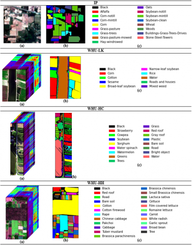
The WHU-HH was procured using the Headwall Nano-Hyperspec imaging sensor. It was deployed atop the DJI M600 Pro UAV platform within Honghu City, positioned in Hubei province, China. The images were captured by the UAV while flying at an elevation of 100 m, resulting in image dimensions measuring 940×475 pixels. These images, acquired by the UAV, possess an approximate spatial resolution of 0.043 m and comprise 270 spectral bands spanning the wavelength spectrum from 400 nm to 1000 nm. This particular dataset embodies various types of the same product, forming a complex agricultural landscape housing numerous product classes [41]. WHU-HH encompasses 22 distinct classes and consists of 386693 samples. Elaborated details regarding WHU-(LK, HC, and HH) and IP can be found in Table 1. Additionally, ground truth information, false-color images, and the color map for all four datasets are provided in Figure 2.
Table 1. Comprehensive data pertaining to the IP, WHU (LK, HC, and HH)
|
No |
IP |
WHU-HC |
WHU-LK |
|||||
|
Classes |
Samples |
Classes |
Samples |
Classes |
Samples |
|||
|
1 |
Alfalfa |
46 |
Strawberry |
44735 |
Corn |
34511 |
||
|
2 |
Corn-notill |
1428 |
Cowpea |
22753 |
Cotton |
8374 |
||
|
3 |
Corn-mintill |
830 |
Soybean |
10287 |
Sesame |
3031 |
||
|
4 |
Corn |
237 |
Sorghum |
5353 |
Broad-leaf soybean |
63212 |
||
|
5 |
Grass-pasture |
483 |
Water spinach |
1200 |
Narrow-leaf soybean |
4151 |
||
|
6 |
Grass-trees |
730 |
Watermelon |
4533 |
Rice |
11854 |
||
|
7 |
Grass-pasture-mowed |
28 |
Greens |
5903 |
Water |
67056 |
||
|
8 |
Hay-windrowed |
478 |
Trees |
17978 |
Roads and houses |
7124 |
||
|
9 |
Oats |
20 |
Grass |
9469 |
Mixed weed |
5229 |
||
|
10 |
Soybean-notill |
972 |
Red roof |
10516 |
|
|
||
|
11 |
Soybean-mintill |
2455 |
Gray roof |
16911 |
|
|
||
|
12 |
Soybean-clean |
593 |
Plastic |
3679 |
|
|
||
|
13 |
Wheat |
205 |
Bare soil |
9116 |
|
|
||
|
14 |
Woods |
1265 |
Road |
18560 |
|
|
||
|
15 |
Buildings-grass-trees-drives |
386 |
Bright object |
1136 |
|
|
||
|
16 |
Stone-steel-towers |
93 |
Water |
75401 |
|
|
||
|
Total Number |
10249 |
|
257530 |
|
204542 |
|||
|
WHU-HH |
||||||||
|
No |
Classes |
Samples |
No |
Classes |
Samples |
|||
|
1 |
Red roof |
14041 |
12 |
Brassica chinensis |
8954 |
|||
|
2 |
Road |
3512 |
13 |
Small Brassica chinensis |
22507 |
|||
|
3 |
Bare soil |
21821 |
14 |
Lactuca sativa |
7356 |
|||
|
4 |
Cotton |
163285 |
15 |
Celtuce |
1002 |
|||
|
5 |
Cotton firewood |
6218 |
16 |
Film covered lettuce |
7262 |
|||
|
6 |
Rape |
44557 |
17 |
Romaine lettuce |
3010 |
|||
|
7 |
Chinese cabbage |
24103 |
18 |
Carrot |
3217 |
|||
|
8 |
Pakchoi |
4054 |
19 |
White radish |
8712 |
|||
|
9 |
Cabbage |
10819 |
20 |
Garlic sprout |
3486 |
|||
|
10 |
Tuber mustard |
12394 |
21 |
Broad beans |
1328 |
|||
|
11 |
Brassica parachinensis |
11015 |
22 |
Tree |
4040 |
|||
|
Total Number |
386693 |
|||||||
2.4 Proposed multipath Hybrid DSCNet
The majority of techniques found in the existing literature for classifying HRSIs are rooted in either 2D CNN, 3D CNN or Hybrid CNN approaches. While 2D CNN can effectively extract spatial features, it tends to overlook the abundant spectral feature data present in HRSIs. Meanwhile, the utilization of 3D CNN introduces heightened computational complexity, which can potentially lead to decreased classification accuracy. Recently, Hybrid CNN methodologies have emerged, merging the strengths of both 2D and 3D CNNs to address challenges associated with both. In this investigation, we propose a distinctive approach - a multipath hybrid 3D/2D Hybrid DSCNet, constructed from layers of 2D and 3D DSC components - designed specifically for HRSIC. The rationale behind adopting DSC layers is as follows:
1. In contrast to the conventional hybrid CNN approach, this method effectively diminishes the count of trainable parameters within the network and concurrently decreases the computation duration. Consequently, the network training process gains speed, while also mitigating the risk of overfitting during classification.
2. Due to their demand for a reduced number of computations, they are associated with lower computational expenses.
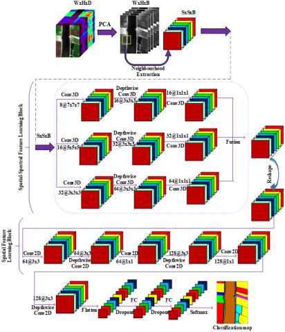
The structure of the Hybrid DSCNet encompasses three components, illustrated in Figure 3. These components are as follows: (1) PCA and the establishment of 3D patches (neighbourhood extraction), (2) the block for learning spatial-spectral features, and (3) the block for learning spatial features.
2.4.1 PCA and the establishment of 3D patches
In the initial phase of the hybrid DSCNet categorization framework, the spatial-spectral HRSI denoted as (X), is portrayed as a three-dimensional cube measuring W×H×D. X stands as the input data for HRSI. W and H symbolize the spatial width and height of the HRSI, while D signifies the count of spectral bands. Each pixel within HRSI encompasses D spectral measurements and constructs a one-hot encoded label array $Y=\left(y_1, y_2, \ldots, y_C\right)$, where C represents the quantity of categories present in the input information. Notwithstanding, the HRSI pixels demonstrate areas of overlap and nesting, substantial similarity between different classes, as well as notable variability within the same class. These aspects call for significant endeavor when employing any classification technique.
Dealing with these issues presents a considerable hurdle for any approach. Addressing these challenges necessitates the elimination of redundant spectral bands. In this pursuit, by utilizing conventional PCA on the HRSI data, the count of bands is adjusted to the desired level. Subsequent to the application of PCA, the spatial dimensions W and H remain unaltered, while the number of spectral bands is diminished from D to B. While PCA retains the spatial dimensions, it curtails the spectral dimension. Following PCA, the HRSI takes on the form of W×H×B, where W denotes width, H signifies height, and B denotes the count of newly acquired bands. To enable classification through DL methods, the HRSI cube is fragmented into compact 3D patches. These 3D patches, measuring S×S×B, are derived from the HRSI cube, centered at spatial coordinates (a,b), and encompassing the spatial dimensions of S×S, as well as all spectral bands in B. The overall count of 3D patches (n) generated from the HRSI cube is determined by (W-S+1)×(H-S+1). Therefore, these sections located at position (a,b) cover the width from $a-(S-1) / 2$ to $a+(S-1) / 2$, the height from $b-(S-1) / 2$ to $b+(S-1) / 2$, and all spectral bands (B) of the HRSI cube [23].
2.4.2 The block for learning spatial-spectral features
During the subsequent phase, inputting 3D hypercubes with dimensions of S×S×B, the spatial-spectral feature learning component comes into play. This component encompasses three distinct strategies for enhancing spatial-spectral features, each involving the integration of 3D CNN and 3D DSC layers. In all three strategies, the initial 3D CNNs exhibit varying filter sizes and kernels. Specifically, the 3D convolution specifications for the 3D CNNs are as follows: 8 filters with a 7×7×7 kernel in the first approach, 16 filters with a 5×5×5 kernel in the second approach, and 32 filters with a 3×3×3 kernel in the third approach. The 3D DSC layers within all three strategies encompass a 3x3x3 DC combined with a 1×1×1 PC. However, the quantity of filters differs for each strategy, being 16, 32, and 64 respectively. As a result, a distinct neural network architecture is tailored for each approach. Leveraging multiple strategies facilitates the extraction of diverse features, thus attaining a more distinct feature representation. Subsequently, these features are consolidated. The feature cubes derived from all three strategies possess identical spatial dimensions, although their depths vary. This is followed by the application of a 3D convolution with dimensions of 1×1×1 and 64 filters, accompanied by a resizing operation.
2.4.3 The block for learning spatial features
In the third phase, operations in the block for learning spatial features are performed after the resizing operation. In order to perform 2D convolution and 2D DSC operations in this block, the input image must be 3D. Therefore, by resizing before this block, the input size is prepared for 2D CNN. In the spatial feature learning block, DSC and 2D CNN are applied to learn more spatial features. Within this module, a 2D convolution with a kernel size of 3×3 and utilizing 64 filters is initially executed on the feature map obtained through the resizing procedure. Then, 64 filters and 3×3 kernel size DC, 64 filters and 1×1 kernel size PC , 128 filters and 3×3 kernel size DC, 128 filters and 1×1 kernel size PC, and finally 128 filters and 3×3 kernel size DC are applied. The features extracted after both feature learning blocks are flattened and given as input to FC layers for HRSIC. The Hybrid DSCNet employs a pair of FC layers, comprising 128 and 256 neurons, respectively. For the purpose of averting overfitting, a dropout layer is introduced following each FC layer, featuring a dropout rate set at 0.4. The outcome from the FC layer is then fed into a basic softmax classifier, yielding the classification outcome. Comprehensive details regarding the Hybrid DSCNet technique are presented in Table 2. The count of parameters available for training in the Hybrid DSCNet technique, in the case of WHU-LK, is 776.089.
Figure 2. (a) Images in false-color representation, (b) maps depicting the ground truth, and (c) color maps associated with the WHU (LK, HC, and HH) and IP
Figure 3. Hybrid 3D-2D depthwise separable convolution networks (Hybrid DSCNet)
Table 2. Detailed information about Hybrid DSCNet for WHU-LK
|
Layer Name |
Layer Details |
Parameters |
Output |
Connected to |
|
InputLayer |
- |
0 |
7×7×20×1 |
- |
|
Conv3D_1a |
filters=8, kernel_size=7×7×7, padding=‘same’ |
2752 |
7×7×20×8 |
InputLayer |
|
Conv3D_1b |
filters=16, kernel_size=5×5×5, padding=‘same’ |
2016 |
7×7×20×16 |
InputLayer |
|
Conv3D_1c |
filters=32, kernel_size=3×3×3, padding=‘same’ |
896 |
7×7×20×32 |
InputLayer |
|
Depthwise_conv3D_1a |
kernel_size=3×3×3, depth_multiplier=2 |
448 |
5×5×18×16 |
Conv3D_1a |
|
Conv3D_2a |
filters=16, kernel_size=1×1×1, padding=‘same’ |
272 |
5×5×18×16 |
Depthwise_conv3D_1a |
|
Depthwise_conv3D_1b |
kernel_size=3×3×3, depth_multiplier=2 |
896 |
5×5×18×32 |
Conv3D_1b |
|
Conv3D_2b |
filters=32, kernel_size=1×1×1, padding=‘same’ |
1056 |
5×5×18×32 |
Depthwise_conv3D_1b |
|
Depthwise_conv3D_1c |
kernel_size=3×3×3, depth_multiplier=2 |
1792 |
5×5×18×64 |
Conv3D_1c |
|
Conv3D_2c |
filters=64, kernel_size=1×1×1, padding=‘same’ |
4160 |
5×5×18×64 |
Depthwise_conv3D_1c |
|
Concatenate |
5×5×18×112 |
Conv3D_2a, Conv3D_2b, Conv3D_2c |
||
|
Conv3D_3a |
filters=64, kernel_size=1×1×1, padding=‘same’ |
7232 |
5×5×18×64 |
Concatenate |
|
Reshape |
- |
0 |
5×5×1152 |
Conv3D_3a |
|
Conv2D_1a |
filters=64, kernel_size=3×3 |
663616 |
3×3×64 |
Reshape |
|
Depthwise_conv2D_1a |
kernel_size=3×3, depth_multiplier=1 |
640 |
3×3×64 |
Conv2D_1a |
|
Conv2D_1b |
filters=64, kernel_size=1×1 |
4160 |
3×3×64 |
Depthwise_conv2D_1a |
|
Depthwise_conv2D_1b |
kernel_size=3×3, depth_multiplier=2 |
1280 |
1×1×128 |
Conv2D_1b |
|
Conv2D_1c |
filters=128, kernel_size=1×1 |
16512 |
1×1×128 |
Depthwise_conv2D_1b |
|
Depthwise_conv2D_1c |
kernel_size=3×3, depth_multiplier=1 |
1280 |
1×1×128 |
Conv2D_1c |
|
Flatten |
- |
0 |
128 |
Depthwise_conv2D_1c |
|
FullyConnected1 (FC) |
units=256 |
33024 |
256 |
Flatten |
|
Dropout_1 |
dropout-ratio 0.4 |
0 |
256 |
FullyConnected1 (FC) |
|
FullyConnected2 (FC) |
units=128 |
32896 |
128 |
Dropout_1 |
|
Dropout_2 |
dropout-ratio 0.4 |
0 |
128 |
FullyConnected2 (FC) |
|
output_layer |
Output_units=9 |
1161 |
9 |
Dropout_2 |
|
Total number of trainable parameters |
776.089 |
|||
3.1 Experimental setup
The experimental studies using the four datasets were written in python using Google Colab. Colab has TPU (Tensor Processing Units) and GPU (Graphics Processing Units) as hardware accelerator. TPU is used in our applications. TPU provides 35GB of RAM and approximately 107GB of storage to run codes. The test-train ratio was taken as 95-5% in all three datasets. Besides, Adam was utilized as the optimizer, and the learning rate was 0.001. Training is performed in 100 epochs and 256 batch sizes. While IP use 25×25 (S=25) window size/patch size for convolution, WHU-LK, WHU-HC and WHU-HH use 7×7 (S=7) window size/patch size. Once PCA is applied to the HRSI data, originally sized WxHxD, the spectral band count is reduced, resulting in a new image size of W×H×B. In various applications, the values selected for B are 30 for IP and 20 for WHU (LK, HC and HH). The dimensions of the 3D patches provided as input to all the DL-based methods employed for comparison are as follows: 7×7×20 for WHU-LK, WHU-HC, WHU-HH and 25×25×30 for IP.
3.2 Evaluation metrics
The assessment of the classification performance of the proposed Hybrid DSCNet across the four datasets was carried out using metrics such as the Average accuracy (AA), Kappa coefficient (K) and Overall accuracy (OA). The calculation of AA involves determining the mean accuracy values on a per-class basis. The OA is expressed as the proportion of accurately classified test samples to the total count of test samples. The K serves as a statistical metric capable of gauging the degree of agreement between the ground truth map and the classification map obtained through estimation.
3.3 Comparison with existing methods and performance analysis
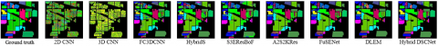
The performance of Hybrid DSCNet was evaluated against eight distinct DL methods introduced in recent years. These methods encompass S3EResBoF [1], A2S2KRes [21], HybridSN [22], FC3DCNN [23], FuSENet [24], DLEM [25], 3D CNN [42], and 2D CNN [43]. The outcomes of the assessments conducted on the IP are presented in Table 3, revealing the classification performance based on both class-specific and overall evaluation metrics (AA, OA, and K). Figure 4 displays the ground truth map alongside the classification maps obtained from the predictive results. Upon reviewing Table 3, it becomes evident that the Hybrid DSCNet achieved the most favorable classification outcomes, boasting an AA of 88.86%, a K value of 93.73%, and an OA of 94.51%. The Hybrid DSCNet method outperforms DLEM, which is one of the methods used for comparison, by 6.74% AA, 3.95% K and 3.43% OA. Similarly, it results in better classification accuracy of 6.42%, 7.31% and 3.77% compared to FuSENet, 4.96%, 5.69% and 2.16% compared to A2S2KRes, 7.25%, 8.26% and 7.77% compared to S3EResBoF, 8.6%, 9.95% and 15.56% compared to HybridSN, 17.62%, 20.3% and 25.56% compared to FC3DCNN, 15.49%, 18.24% and 28.15% compared to 3D CNN, 19.26%, 22.45% and 26.33% compared to 2D CNN. The least favorable outcomes were observed in the case of 2D CNN, yielding an OA of 75.25% and a K value of 71.28%. Similarly, 3D CNN exhibited suboptimal performance, registering an AA of 60.71%. The AA outcome from the 3D CNN demonstrates a situation where the class-specific classification results exhibit a notably diminished level of accuracy for each individual class. Considering the accuracies for individual classes, it becomes evident that the Hybrid DSCNet method yielded the most superior classification outcomes for classes 2, 3, 4, 5, 6, 8, 12, and 14, showcasing values of 93.66%, 91.38%, 95.55%, 98.47%, 95.67%, 100%, 94.14%, and 99.92% respectively. In the case of class 7 and 16, the highest accuracy in classification was achieved through the utilization of the FuSENet and S3EResBoF methods, both attaining a perfect 100% accuracy. The highest classification accuracies for class 10 and 11 were obtained in DLEM with 92.36% and 97.56%, respectively. The highest classification performances were obtained in FuSENet with 100% for class 1, HybridSN with 78.95% for class 9, FC3DCNN with 98.38% for class 13 and S3EResBoF with 98.41% for class 15. Furthermore, the durations for both training and testing across all methodologies are presented in Table 3. The training duration is expressed in minutes, while the testing duration is quantified in seconds. Upon analyzing the training and testing durations of the eight distinct approaches, it is evident that the Hybrid DSC approach, as proposed, exhibited comparatively swifter training and testing procedures in comparison to the other seven methodologies, with the exception of 2D CNN. The reason why it is lower in 2D CNN is due to the inability to obtain spectral feature information.
Upon conducting assessments on the WHU-LK, the outcomes of the classifications, considering both class-specific and comprehensive evaluation metrics (AA, OA, and K), are detailed in Table 4. The visual representation of the ground truth map alongside the classification maps within the predictive outcome is illustrated in Figure 5. Based on the data in Table 4, it is evident that the most favorable classification outcomes were achieved by the Hybrid DSCNet, showcasing an impressive 99.36% AA, 99.72% K, and 99.78% OA. The closest classification results to the Hybrid DSCNet were obtained in DLEM with 99.20% AA, 99.68% K, 99.76% OA and in A2S2KRes with 99.21% AA, 99.51% K and 99.63% OA. The classification results (AA, K and OA) obtained by other methods are as follows: 99.18%, 99.40%, 99.54% with FuSENet, 99.11%, 99.52%, 99.63% with HybridSN, 99.07%, 99.64%, 99.64% with FC3DCNN, 98.96%, 99.46%, 99.59% with S3EResBoF, 98.79%, 99.46%, 99.59% with 3D CNN, 98.09%, 99.24%, 99.42% with 2D CNN. The worst AA result was acquire with 2D CNN. According to class-wise classification accuracies, the classification results of 100%, 99.91%, 100% and 98.76% were obtained in the 3, 4, 6 and 8 classes, respectively, with the proposed Hybrid DSCNet method. The proposed approach demonstrates its superiority across these specific classes, delivering the most impressive results. Notably, the DLEM exhibited the highest classification performance, boasting an impressive 99.99% and 99.89% accuracy for class 1 and 2, respectively. In similar fashion, A2S2KRes achieved 99.84% accuracy for class 5, FuSENet excelled with 99.99% accuracy for class 7, and S3EResBoF attained a notable 99.55% accuracy for class 9. With the exception of classes 3, 4, 6, and 8, the proposed Hybrid DSCNet method approached the performance of the top-performing method across the remaining classes. The training and testing durations of the methods using the WHU-LK are presented in Table 4. Upon analyzing Table 4, it becomes apparent that the proposed Hybrid DSC method exhibited faster training and testing processes than other methods, excluding the 2D CNN. Factoring in all the information from Table 4, it is evident that the Hybrid DSCNet method achieves enhanced classification outcomes within a shorter time frame.
Table 3. The outcomes of classification achieved through the utilization of the IP dataset (%)
|
No |
Train/Test |
2D CNN |
3D CNN |
FC3DCNN |
HybridSN |
S3EResBoF |
A2S2KRes |
FuSENet |
DLEM |
Hybrid DSCNet |
|
1 |
2/44 |
26.67 |
22.22 |
26.83 |
40.00 |
0.0 |
81.19 |
100 |
55.55 |
59.09 |
|
2 |
71/1357 |
75.31 |
69.17 |
70.27 |
89.60 |
77.39 |
83.86 |
92.41 |
88.74 |
93.66 |
|
3 |
41/789 |
48.82 |
64.10 |
66.13 |
70.81 |
74.94 |
82.97 |
85.25 |
89.69 |
91.38 |
|
4 |
12/225 |
23.48 |
3.04 |
50.23 |
50.00 |
90.70 |
91.23 |
90.91 |
53.91 |
95.55 |
|
5 |
24/459 |
48.19 |
72.07 |
77.01 |
68.66 |
97.03 |
93.77 |
96.32 |
83.58 |
98.47 |
|
6 |
37/693 |
91.10 |
95.20 |
84.93 |
90.68 |
88.79 |
94.11 |
83.14 |
90.54 |
95.67 |
|
7 |
1/27 |
62.96 |
11.11 |
8.00 |
51.85 |
100 |
84.73 |
100 |
62.96 |
96.30 |
|
8 |
24/454 |
83.62 |
100 |
98.84 |
100 |
100 |
96.09 |
100 |
100 |
100 |
|
9 |
1/19 |
89.47 |
21.05 |
5.56 |
78.95 |
28.81 |
43.45 |
22.22 |
68.42 |
42.10 |
|
10 |
49/923 |
74.23 |
78.15 |
86.40 |
87.38 |
75.63 |
88.96 |
78.03 |
92.36 |
91.66 |
|
11 |
123/2332 |
88.41 |
96.30 |
79.91 |
96.85 |
96.31 |
91.54 |
91.33 |
97.56 |
95.32 |
|
12 |
30/563 |
62.78 |
64.00 |
49.62 |
66.09 |
88.55 |
86.41 |
81.86 |
77.74 |
94.14 |
|
13 |
10/195 |
77.39 |
85.43 |
98.38 |
83.92 |
84.95 |
91.24 |
60.36 |
85.93 |
92.82 |
|
14 |
63/1202 |
99.92 |
90.79 |
90.08 |
96.49 |
95.96 |
95.29 |
96.32 |
98.70 |
99.92 |
|
15 |
19/367 |
33.69 |
38.77 |
61.09 |
66.04 |
98.41 |
95.74 |
83.29 |
89.30 |
82.56 |
|
16 |
5/88 |
14.44 |
60.00 |
59.52 |
35.55 |
100 |
86.61 |
100 |
78.89 |
93.18 |
|
OA |
512 / 9737 |
75.25 |
79.02 |
76.89 |
85.91 |
87.26 |
89.55 |
88.09 |
91.08 |
94.51 |
|
K |
71.28 |
75.49 |
73.43 |
83.78 |
85.47 |
88.04 |
86.42 |
89.78 |
93.73 |
|
|
AA |
62.53 |
60.71 |
63.30 |
73.30 |
81.09 |
86.70 |
85.09 |
82.12 |
88.86 |
|
|
Training Time (min.) |
1.27 |
54.1 |
18.3 |
14.1 |
10.96 |
7.22 |
13.3 |
9.55 |
1.5 |
|
|
Testing Time (sec.) |
1 |
4.26 |
4.7 |
4.8 |
3 |
12 |
3.99 |
3.15 |
1.2 |
|
Figure 4. The classification maps derived from the estimation process for the IP
Table 4. The outcomes of classification achieved through the utilization of the WHU-LK dataset (%)
|
No |
Train/Test |
2D CNN |
3D CNN |
FC3D CNN |
HybridSN |
S3EResBoF |
A2S2KRes |
FuSENet |
DLEM |
Hybrid DSCNet |
|
1 |
1725/32786 |
99.95 |
99.89 |
99.90 |
99.99 |
99.97 |
99.31 |
99.83 |
99.99 |
99.90 |
|
2 |
419/7955 |
98.89 |
99.20 |
99.26 |
99.87 |
99.01 |
99.30 |
99.42 |
99.89 |
99.68 |
|
3 |
152/2879 |
97.48 |
99.83 |
99.76 |
98.98 |
100 |
99.13 |
99.82 |
99.42 |
100 |
|
4 |
3161/60051 |
99.67 |
99.71 |
99.62 |
99.46 |
99.88 |
99.81 |
99.31 |
99.85 |
99.91 |
|
5 |
207/3944 |
97.07 |
98.46 |
97.76 |
97.59 |
99.46 |
99.84 |
99.54 |
98.34 |
98.73 |
|
6 |
593/11261 |
99.57 |
99.86 |
99.92 |
99.88 |
99.99 |
99.63 |
99.97 |
99.87 |
100 |
|
7 |
3353/63703 |
99.98 |
99.97 |
99.98 |
99.96 |
99.88 |
99.98 |
99.99 |
99.98 |
99.93 |
|
8 |
356/6768 |
95.45 |
98.16 |
98.41 |
98.16 |
92.85 |
98.26 |
95.79 |
98.36 |
98.76 |
|
9 |
261/4968 |
94.75 |
94.08 |
97.06 |
98.13 |
99.55 |
97.64 |
98.91 |
97.08 |
97.40 |
|
OA |
10227 / 194315 |
99.42 |
99.59 |
99.64 |
99.63 |
99.59 |
99.63 |
99.54 |
99.76 |
99.78 |
|
K |
99.24 |
99.46 |
99.64 |
99.52 |
99.46 |
99.51 |
99.40 |
99.68 |
99.72 |
|
|
AA |
98.09 |
98.79 |
99.07 |
99.11 |
98.96 |
99.21 |
99.18 |
99.20 |
99.36 |
|
|
Training Time (min.) |
1.63 |
2.7 |
4.1 |
6.33 |
10.54 |
29.38 |
13.8 |
19 |
2.6 |
|
|
Testing Time (sec.) |
10.3 |
19 |
26 |
29 |
36 |
47.7 |
37 |
20.1 |
10.5 |
|
Figure 5. The classification maps derived from the estimation process for the WHU-LK
Table 5. The outcomes of classification achieved through the utilization of the WHU-HC dataset (%)
|
No |
Train/Test |
2D CNN |
3D CNN |
FC3D CNN |
HybridSN |
S3EResBoF |
A2S2KRes |
FuSENet |
DLEM |
Hybrid DSCNet |
|
1 |
2237/42498 |
96.61 |
96.80 |
98.46 |
97.19 |
91.61 |
95.26 |
97.49 |
98.41 |
98.24 |
|
2 |
1137/21616 |
93.65 |
93.14 |
95.73 |
94.38 |
95.07 |
97.44 |
97.16 |
96.69 |
96.44 |
|
3 |
514/9773 |
86.85 |
91.03 |
89.49 |
89.96 |
92.12 |
94.71 |
99.09 |
94.38 |
95.74 |
|
4 |
268/5085 |
98.21 |
97.82 |
98.46 |
98.28 |
98.14 |
97.67 |
99.61 |
98.77 |
98.74 |
|
5 |
60/1140 |
69.59 |
67.18 |
74.74 |
61.43 |
96.94 |
89.86 |
87.30 |
90.55 |
87.46 |
|
6 |
227/4306 |
68.41 |
67.36 |
69.82 |
70.00 |
79.46 |
78.51 |
57.36 |
75.96 |
82.05 |
|
7 |
295/5608 |
88.02 |
90.24 |
87.53 |
87.63 |
93.61 |
91.80 |
93.58 |
93.24 |
94.65 |
|
8 |
899/17079 |
87.54 |
90.41 |
94.72 |
91.68 |
94.11 |
92.96 |
92.87 |
95.30 |
96.58 |
|
9 |
473/8996 |
89.13 |
89.01 |
90.58 |
92.75 |
92.31 |
92.99 |
91.03 |
94.28 |
94.72 |
|
10 |
526/9990 |
99.01 |
97.80 |
98.13 |
98.99 |
98.33 |
98.84 |
96.78 |
98.67 |
99.01 |
|
11 |
845/16066 |
96.74 |
96.96 |
98.85 |
98.25 |
92.37 |
96.42 |
94.90 |
97.51 |
98.70 |
|
12 |
184/3495 |
66.74 |
87.31 |
80.44 |
69.36 |
84.98 |
84.95 |
57.56 |
82.18 |
87.87 |
|
13 |
456/8660 |
77.10 |
75.30 |
81.08 |
75.67 |
76.54 |
86.51 |
67.25 |
84.27 |
86.81 |
|
14 |
928/17632 |
90.05 |
91.82 |
87.45 |
91.65 |
91.31 |
98.42 |
98.74 |
94.68 |
96.25 |
|
15 |
57/1079 |
57.89 |
73.23 |
84.94 |
72.41 |
96.10 |
91.42 |
97.43 |
84.93 |
79.70 |
|
16 |
3770/71631 |
99.33 |
99.73 |
99.71 |
99.38 |
99.95 |
99.78 |
99.65 |
99.76 |
99.76 |
|
OA |
12876 / 244654 |
93.40 |
94.28 |
95.09 |
94.41 |
94.27 |
96.87 |
94.05 |
96.47 |
97.06 |
|
K |
92.28 |
93.30 |
94.25 |
93.45 |
93.28 |
96.34 |
93.05 |
95.87 |
96.56 |
|
|
AA |
85.30 |
87.82 |
89.38 |
86.94 |
92.06 |
92.97 |
89.24 |
92.47 |
93.30 |
|
|
Training Time (min.) |
1.7 |
4.40 |
4.5 |
4.71 |
11 |
26.05 |
12.17 |
29 |
3.47 |
|
|
Testing Time (sec.) |
19 |
23 |
23.3 |
43 |
37 |
117 |
37 |
60 |
20.3 |
|
Figure 6. The classification maps derived from the estimation process for the WHU-HC
Upon conducting experiments on the WHU-HC, the outcomes of the classification are depicted in Table 5, presenting evaluations based on class-specific and overall criteria (AA, OA, and K). The classification outcomes, alongside the ground truth map and classification maps, are visually presented in Figure 6 for all methods in the prediction results. Upon reviewing Table 5, it becomes evident that the most favorable classification outcomes were attained using the Hybrid DSCNet, yielding an AA of 93.30%, K of 96.56%, and OA of 97.06%. The Hybrid DSCNet yielded the most similar classification outcomes, closely followed by DLEM at 92.47%, 95.87%, and 96.47%, and A2S2KRes with 92.97%, 96.34%, and 96.87%, when evaluating AA, K, and OA classification criteria. The classification metrics (AA, K, and OA) obtained from other techniques are as follows: 92.06%, 93.28%, 94.27% with S3EResBoF, 89.24%, 93.05%, 94.05% with FuSENet, 89.38%, 94.25%, 95.09% with FC3DCNN, 87.82%, 93.30%, 94.28% with 3D CNN, 86.94%, 93.45%, 94.41% with HybridSN, and 85.30%, 92.28%, 93.40% with 2D CNN. Analyzing all methods reveals that the least favorable classification results are obtained with the utilization of 2D CNN. According to class-wise classification accuracies, the classification results of 82.05%, 94.65%, 96.58%, 94.72%, 99.01%, 87.87% and 86.81% were obtained in the 6, 7, 8, 9, 10, 12 and 13 classes, respectively, with the proposed Hybrid DSCNet method.
Among these classes, the Hybrid DSCNet approach delivers the most favorable classification outcomes. The top classification accuracy was achieved by the FuSENet technique, attaining 99.09%, 99.61%, 98.74%, and 97.43% for class 3, 4, 14, and 15, respectively. The highest classification results was obtained in the FC3DCNN with 98.46% and 98.85% for class 1 and 11, in the S3EResBoF method with 96.94% and 99.95% for class 5 and 16, in the A2S2KRes method with 96.94% for class 2. Except for the 3, 5, 14 and 15 classes, the proposed Hybrid DSCNet method in other classes acquired a classification result close to the method that gave the highest classification result. Furthermore, the training and testing durations for all approaches are displayed in Table 5. Analyzing the data in Table 5 reveals that, except for the 2D CNN method, the proposed Hybrid DSCNet technique exhibits faster training and testing times than other sophisticated methods. Taking into account the comprehensive details presented in Table 5, it can be inferred that the Hybrid DSCNet method attains superior classification outcomes in a more efficient timeframe.
Table 6. The outcomes of classification achieved through the utilization of the WHU-HH dataset (%)
|
No |
Train/Test |
2D CNN |
3D CNN |
FC3D CNN |
HybridSN |
S3EResBoF |
A2S2KRes |
FuSENet |
DLEM |
Hybrid DSCNet |
|
1 |
702/13339 |
98.41 |
98.05 |
98.05 |
97.60 |
93.77 |
99.28 |
99.34 |
97.94 |
98.78 |
|
2 |
176/3336 |
83.97 |
89.87 |
70.32 |
86.32 |
95.38 |
94.70 |
84.14 |
94.83 |
94.84 |
|
3 |
1091/20730 |
95.75 |
92.26 |
97.77 |
95.38 |
95.17 |
97.56 |
96.03 |
98.08 |
97.76 |
|
4 |
8164/155121 |
99.30 |
99.47 |
99.12 |
99.34 |
99.59 |
99.40 |
98.15 |
99.89 |
99.70 |
|
5 |
311/5907 |
78.36 |
71.53 |
81.22 |
57.72 |
52.48 |
91.65 |
88.43 |
78.25 |
90.89 |
|
6 |
2228/42329 |
97.13 |
97.31 |
97.89 |
96.98 |
98.52 |
98.95 |
97.77 |
98.26 |
98.22 |
|
7 |
1205/22898 |
90.16 |
90.70 |
95.65 |
88.30 |
98.24 |
93.99 |
94.47 |
95.92 |
95.80 |
|
8 |
203/3851 |
60.73 |
63.50 |
76.19 |
47.30 |
86.02 |
87.18 |
83.29 |
68.97 |
81.04 |
|
9 |
541/10278 |
97.69 |
97.90 |
99.32 |
98.11 |
100 |
99.29 |
99.38 |
99.01 |
98.42 |
|
10 |
620/11774 |
88.19 |
82.52 |
88.96 |
71.34 |
90.06 |
95.95 |
94.63 |
89.58 |
92.93 |
|
11 |
551/10464 |
84.29 |
82.31 |
85.93 |
75.27 |
82.45 |
93.14 |
89.65 |
90.90 |
91.98 |
|
12 |
448/8506 |
69.24 |
74.66 |
81.22 |
77.96 |
73.33 |
91.97 |
74.18 |
89.64 |
88.67 |
|
13 |
1125/21382 |
83.26 |
87.44 |
88.58 |
78.65 |
82.91 |
91.39 |
90.46 |
88.97 |
94.31 |
|
14 |
368/6988 |
92.35 |
91.74 |
95.35 |
90.22 |
99.20 |
96.73 |
99.05 |
93.29 |
95.92 |
|
15 |
50/952 |
71.60 |
80.14 |
85.18 |
91.36 |
50.10 |
92.21 |
99.71 |
93.31 |
82.67 |
|
16 |
363/6899 |
94.46 |
95.00 |
97.61 |
93.03 |
98.73 |
98.22 |
99.13 |
96.14 |
97.82 |
|
17 |
150/2860 |
87.57 |
89.83 |
77.12 |
87.16 |
76.87 |
97.96 |
92.86 |
96.74 |
89.47 |
|
18 |
161/3056 |
92.57 |
95.39 |
97.66 |
89.14 |
91.77 |
90.08 |
83.03 |
97.56 |
96.24 |
|
19 |
435/8277 |
90.85 |
92.59 |
93.35 |
88.26 |
89.79 |
94.69 |
98.53 |
93.99 |
95.52 |
|
20 |
174/3312 |
82.64 |
90.09 |
91.36 |
75.24 |
91.32 |
94.71 |
98.01 |
93.37 |
94.38 |
|
21 |
66/1262 |
34.24 |
76.94 |
44.72 |
43.71 |
50.26 |
64.35 |
55.78 |
39.13 |
91.52 |
|
22 |
202/3838 |
90.69 |
87.88 |
95.25 |
85.68 |
90.81 |
92.79 |
81.42 |
89.72 |
97.24 |
|
OA |
19334 / 367359 |
93.81 |
94.12 |
95.38 |
92.15 |
93.54 |
97.10 |
95.51 |
96.31 |
97.27 |
|
K |
92.17 |
92.56 |
95.38 |
90.05 |
91.90 |
96.34 |
94.31 |
95.33 |
96.54 |
|
|
AA |
84.70 |
87.60 |
88.08 |
82.46 |
85.76 |
93.46 |
90.79 |
90.16 |
93.82 |
|
|
Training Time (min.) |
2.64 |
19.78 |
13.48 |
11.12 |
24.07 |
43.9 |
27.75 |
47 |
5.42 |
|
|
Testing Time (sec.) |
65 |
334 |
269 |
195 |
126.5 |
341 |
254 |
277 |
119 |
|
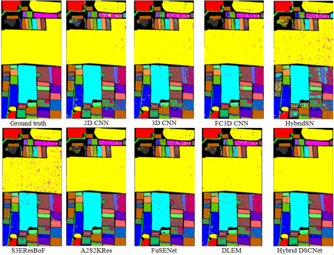
Figure 7. The classification maps derived from the estimation process for the WHU-HH
Upon conducting the experiments on the WHU-HH, the classification outcomes are detailed in Table 6, encompassing both class-specific and overall evaluation criteria (AA, OA, and K). Additionally, Figure 7 exhibits the ground truth map and the classification maps produced by various methods for predicting results. Upon scrutinizing Table 6, it becomes evident that the Hybrid DSCNet demonstrated superior classification accuracies, achieving 93.82% for AA, 96.54% for K, and 97.27% for OA. The proposed Hybrid DSCNet method outperforms A2S2KRes, which is one of the methods used for comparison, by 0.36% AA, 0.2% K and 0.17% OA. Similarly, it results in better classification accuracies of 1.76%, 2.23% and 3.03% compared to FuSENet, 0.96%, 1.21% and 3.66% compared to DLEM, 3.73%, 4.64% and 8.06% compared to S3EResBoF, 5.12%, 6.49% and 11.36% compared to HybridSN, 1.89%, 1.16% and 5.74% compared to FC3DCNN, 3.15%, 3.98% and 6.22% compared to 3D CNN, 3.46%, 4.37% and 9.12% compared to 2D CNN. Considering all methods, it is seen that the closest classification results to the Hybrid DSCNet are obtained with A2S2KRes. Upon analyzing the classification outcomes on a class-wise basis, it is evident that the Hybrid DSCNet method achieved the most favorable classification results in classes 5, 11, 13, 21, and 22, attaining accuracies of 90.89%, 91.98%, 94.31%, 91.52%, and 97.24%, respectively. The highest classification results for class 1, 15, 16, 19 and 20 were acquired in FuSENet with 99.34%, 99.71%, 99.13%, 98.53% and 98.01%. The highest classification results were obtained in S3EResBoF with 95.38%, 98.24%, 100%, 99.20% for class 2, 7, 9,14, DLEM with 98.08% and 99.89% for class 3 and 4, FC3DCNN with 97.66% for class 18 and A2S2KRes with 98.95%, 87.18%, 95.95%, 91.97%, 97.96% for class 6, 8, 10, 12, 17. Based on the data presented in Table 6, it is evident that the Hybrid DSCNet approach requires less time for training and testing when compared to other sophisticated methods, excluding the 2D CNN. Taking into account all the details provided in Table 6, it can be inferred that the proposed method yields improved classification results within a shorter timeframe.
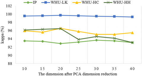
Figure 8. OA, AA, and K values obtained with different principal components for the four datasets
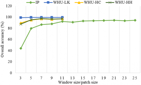
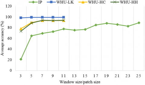
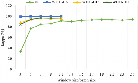
Figure 9. Effect of different spatial patch sizes on classification accuracy with 5% training samples on IP, WHU-LK, WHU-HC and WHU-HH datasets
In the Hybrid DSCNet method, classification accuracies were tested with different principal components in four different datasets to determine the number of principal components obtained after PCA dimension reduction method. Seven different principal component cases between 10 and 40 are considered in all datasets and classification accuracies for all principal components are given in Figure 8. When the classification accuracies in Figure 8 are examined, the number of reduced spectral bands after PCA in the proposed Hybrid DSCNet method was determined as 30, 20, 20 and 20 for IP, WHU-LK, WHU-HC and WHU-HH, respectively.
For the Hybrid DSCNet method, the effect of different spatial dimensions on the classification accuracies in four different datasets was analyzed and given in Figure 9. While only 3×3, 5×5, 7×7, 9×9 and 11×11 spatial dimensions (patch size) are taken into account in WHU-LK, WHU-HC and WHU-HH datasets, 12 different cases are tested between 3×3 and 25×25 spatial dimensions in IP. With increasing the spatial dimension in the WHU-LK, WHU-HC and WHU-HH datasets, the training time of the proposed method increases significantly. In addition, the need for graphics memory and internal memory are also increasing. To make a fair comparison and balance computational cost and accuracy, we determined the same spatial dimension of 7×7×B across all WHU-LK, WHU-HC, WHU-HH datasets. In the IP dataset, the most appropriate spatial patch size is 25×25. Because the best classification accuracies was obtained with the spatial patch size of 25×25.
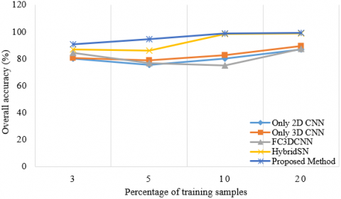
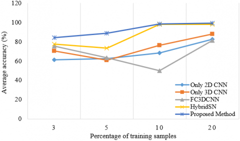
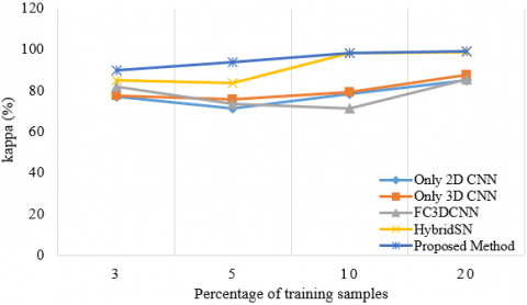
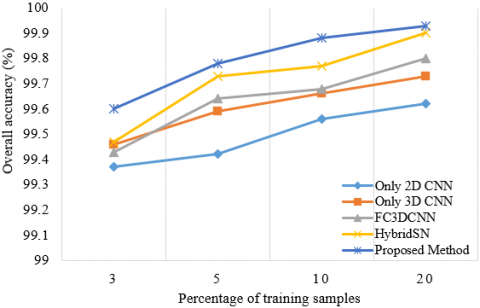
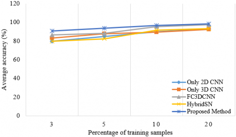
Figures 10-13 show that studies were carried out by taking different training samples (3%, 5%, 10% and 20%) for four datasets. The classification accuracies of the Hybrid DSCNet, 2D CNN, 3D CNN, HybridSN, FC3DCNN with different training examples in all datasets were examined. According to Figures 10-13, it is seen that the Hybrid DSCNet provides better classification accuracies than all methods as the number of training samples increases. Especially for complex scenes in WHU-HC and WHU-HH, the Hybrid DSCNet shows a more important advantage than other classifiers.
Figure 10. OA, AA and K values of different numbers of training samples for only 2D CNN, only 3D CNN, FC 3D CNN, HybridSN and the proposed method on IP dataset
Figure 11. OA, AA and K values of different numbers of training samples for only 2D CNN, only 3D CNN, FC 3D CNN, HybridSN and the proposed method on WHU-LK dataset
Figure 12. OA, AA and K values of different numbers of training samples for only 2D CNN, only 3D CNN, FC 3D CNN, HybridSN and the proposed method on WHU-HC dataset
Figure 13. OA, AA and K values of different numbers of training samples for only 2D CNN, only 3D CNN, FC 3D CNN, HybridSN and the proposed method on WHU-HH dataset
In this paper, Hybrid DSCNet based on multipath feature fusion is suggested for HRSI classification. With the Hybrid DSCNet, it is purposed to improve the classification results by decreasing the number of trainable parameters. In this direction, unlike the Hybrid CNN methods used in the literature, 3D-2D depthwise and pointwise convolution layers are used instead of standard 3D-2D CNN. With these layers, the number of trainable parameters is reduced and the classification performance is increased. In addition, a multipath feature fusion structure is created to extract more spatial-spectral and spatial features. Thanks to a multi-scale network structure, the features extracted from HRSI are getting richer. Classification results of the Hybrid DSCNet on IP, WHU (LK, HC and HH) datasets were examined. Using 5% training sample with IP, WHU-LK, WHU-HC and WHU-HH, OA values of 94.51%, 99.78%, 97.06% and 97.27% were acquired. In addition, the Hybrid DSCNet was compared with the latest technology methods from the literature. It has been seen that the Hybrid DSCNet produces successful classification performances. When the classification results obtained are examined, it is concluded that the Hybrid DSCNet can be used in real world applications. In the future, studies based on Generative Adversarial Networks, Vision transformer, Swin Transformer, ConvMixer are planned for HRSIC. With these methods, it is aimed to further increase the classification accuracy results.
|
CNN |
Convolutional Neural Networks |
|
HRSI |
Hyperspectral Remote Sensing Images |
|
DRM PCA |
Dimension Reduction Methods Principal Component Analysis |
|
LDA |
Linear Discriminant Analysis |
|
ICA |
Independent Component Analysis |
|
IPCA |
Incremental Principal Component Analysis |
|
LLE |
Locally Linear Embedding |
|
SVM |
Support Vector Machine |
|
KNN |
K-Nearest-Neighbors |
|
DL |
Deep Learning |
|
IP |
Indian Pines |
|
WHU-LK |
WHU-Hi-Longkou |
|
WHU-HC |
WHU-Hi-Hanchuan |
|
WHU-HH |
WHU-Hi-Honghu |
|
DC |
Depthwise convolution |
|
PC |
Pointwise convolution |
|
UAV |
Unmanned Aerial Vehicle |
|
ANN |
Artificial Neural Networks |
|
FE |
Feature Extraction |
|
DNN |
Deep Neural Network |
[1] Roy, S.K., Chatterjee, S., Bhattacharyya, S., Chaudhuri, B.B., Platos, J. (2020). Lightweight spectral-spatial squeeze-and- excitation residual bag-of-features learning for hyperspectral classification. IEEE Transactions on Geoscience and Remote Sensing, 58(8): 5277-5290. https://doi.org/10.1109/TGRS.2019.2961681
[2] Wang, A., Liu, C., Xue, D., Wu, H., Zhang, Y., Liu, M. (2021). Depthwise separable relation network for small sample hyperspectral image classification. Symmetry (Basel), 13(9): 1673. https://doi.org/10.3390/sym13091673
[3] Ahmad, M., Mazzara, M., Distefano, S. (2021). Regularized CNN feature hierarchy for hyperspectral image classification. Remote Sensing, 13(12): 1-11. https://doi.org/10.3390/rs13122275
[4] Firat, H., Hanbay, D. (2021). 3B ESA tabanlı ResNet50 kullanilarak hiperspektral görüntülerin siniflandirilmasi classification of hyperspectral images using 3D CNN based ResNet50. 29th Signal Processing and Communications Applications Conference (SIU), pp. 6-9. https://doi.org/10.1109/SIU53274.2021.9477899
[5] Cao, F., Guo, W. (2020). Deep hybrid dilated residual networks for hyperspectral image classification. Neurocomputing, 384: 170-181. https://doi.org/10.1016/j.neucom.2019.11.092
[6] Fırat, H., Hanbay, D. (2022). 4CF-Net: New 3D convolutional neural network for spectral spatial classification of hyperspectral remote sensing images. Journal of the Faculty of Engineering and Architecture of Gazi University, 37(1): 439-453. https://doi.org/10.17341/gazimmfd.901291
[7] Firat, H., Asker, M.E., Bayindir, M.İ., Hanbay, D. (2022). 3D residual spatial–spectral convolution network for hyperspectral remote sensing image classification. Neural Computing and Applications, 8. https://doi.org/10.1007/s00521-022-07933-8
[8] Ahmad, M., Shabbir, S., Raza, R.A., Mazzara, M., Distefano, S., Khan, A.M. (2021). Artifacts of different dimension reduction methods on hybrid CNN feature hierarchy for Hyperspectral Image Classification. Optik, 246: 167757. https://doi.org/10.1016/j.ijleo.2021.167757
[9] Firat, H., Asker, M.E., Hanbay, D. (2022). Classification of hyperspectral remote sensing images using different dimension reduction methods with 3D/2D CNN. Remote Sensing Applications: Society and Environment, 100694. https://doi.org/10.1016/j.rsase.2022.100694
[10] Mohan, A., Venkatesan, M. (2020). HybridCNN based hyperspectral image classification using multiscale spatiospectral features. Infrared Physics & Technology, 108. https://doi.org/10.1016/j.infrared.2020.103326
[11] Mohan, A., Meenakshi Sundaram, V. (2020). V3O2: Hybrid deep learning model for hyperspectral image classification using vanilla-3D and octave-2D convolution. Journal of Real-Time Image Processing, 18: 1681-1695. https://doi.org/10.1007/s11554-020-00966-z
[12] Wang, Y., Yu, W., Fang, Z. (2020). Multiple Kernel-based SVM classification of hyperspectral images by combining spectral, spatial, and semantic information. Remote Sensing, 12(1). https://doi.org/10.3390/RS12010120
[13] Li, J., Bioucas-Dias, J.M., Plaza, A. (2010). Semisupervised hyperspectral image segmentation using multinomial logistic regression with active learning. IEEE Transactions on Geoscience and Remote Sensing, 48(11): 4085-4098. https://doi.org/10.1109/TGRS.2010.2060550
[14] Ahmad., M. (2019). Spatial prior fuzziness pool-based interactive classification of hyperspectral images. Remote Sensing, 11(9): 1-19. https://doi.org/10.3390/rs11091136
[15] Palmason, J.A., Benediktsson, J.A., Sveinsson, J.R. (2005). Classification of hyperspectral data from urban areas based on extended morphological profiles. IEEE Transactions on Geoscience and Remote Sensing, 43(3): 480-491. https://doi.org/10.1109/TGRS.2004.842478
[16] Camps-Valls., G., Bruzzone., L. (2005). Kernel-based methods for hyperspectral image classification. IEEE Transactions on Geoscience and Remote Sensing, 43(6): 1351-1362. https://doi.org/10.1109/TGRS.2005.846154
[17] Fang, L., Li, S., Duan, W., Ren, J., Benediktsson, J.A. (2015). Classification of hyperspectral images by exploiting spectral-spatial information of superpixel via multiple kernels. IEEE Transactions on Geoscience and Remote Sensing, 53(12): 6663-6674. https://doi.org/10.1109/TGRS.2015.2445767
[18] Fang, L., Li, S., Kang, X., Benediktsson, J.A. (2014). Spectral-spatial hyperspectral image classification via multiscale adaptive sparse representation. IEEE Transactions on Geoscience and Remote Sensing, 52(12): 7738-7749. https://doi.org/10.1109/TGRS.2014.2318058
[19] Uzen, H., Turkoglu, M., Hanbay, D. (2021). Texture defect classification with multiple pooling and filter ensemble based on deep neural network. Expert Systems with Applications, 175: 114838. https://doi.org/10.1016/j.eswa.2021.114838
[20] Zhang, C. (2019). Joint deep learning for land cover and land use classification. Remote Sensing of Environment, 221: 173-187. https://doi.org/10.1016/j.rse.2018.11.014
[21] Roy, S.K., Manna, S., Song, T., Bruzzone, L. (2020). Attention-based adaptive spectral-spatial kernel ResNet for hyperspectral image classification. IEEE Transactions on Geoscience and Remote Sensing, 59(9): 7831-7843. https://doi.org/10.1109/TGRS.2020.3043267
[22] Roy, S.K., Krishna, G., Dubey, S.R., Chaudhuri, B.B. (2019). HybridSN: Exploring 3D-2D CNN feature hierarchy for hyperspectral image classification. arXiv, 17(2): 277-281. https://doi.org/10.1109/LGRS.2019.2918719
[23] Ahmad, M., Khan, A.M., Mazzara, M., Distefano, S., Ali, M., Sarfraz, M.S. (2020). A fast and compact 3-D CNN for hyperspectral image classification. IEEE Geoscience and Remote Sensing Letters, 19: 1-5. https://doi.org/10.1109/LGRS.2020.3043710
[24] Roy, S.K., Dubey, S.R., Chatterjee, S., Chaudhuri, B.B. (2020). FuSENet: Fused squeeze-and-excitation network for spectral-spatial hyperspectral image classification. IET Image Processing, 14(8): 1653-1661. https://doi.org/10.1049/iet-ipr.2019.1462
[25] Iyer, P., Sriram, A., Lal, S. (2021). Deep learning ensemble method for classification of satellite hyperspectral images. Remote Sensing Applications: Society and Environment, 23: 100580. https://doi.org/10.1016/j.rsase.2021.100580
[26] Xu, H., Yao, W., Cheng, L., Li, B. (2021). Multiple spectral resolution 3D convolutional neural network for hyperspectral image classification. Remote Sensing, 13(7). https://doi.org/10.3390/rs13071248
[27] Gao, H., Yang, Y., Li, C., Gao, L., Zhang, B. (2021). Multiscale residual network with mixed depthwise convolution for hyperspectral image classification. IEEE Transactions on Geoscience and Remote Sensing, 59(4): 3396-3408. https://doi.org/10.1109/TGRS.2020.3008286
[28] Fırat, H., Asker, M.E., Hanbay, D. (2022). Hybrid 3D convolution and 2D depthwise separable convolution neural network for hyperspectral image classification. Balkan Journal of Electrical and Computer Engineering, 10(1): 35-46. https://doi.org/10.17694/bajece.1039029
[29] Zheng, J., Feng, Y., Bai, C., Zhang, J. (2021). Hyperspectral image classification using mixed convolutions and covariance pooling. IEEE Transactions on Geoscience and Remote Sensing, 59(1): 522-534. https://doi.org/10.1109/TGRS.2020.2995575
[30] Sun, H., Zheng, X., Lu, X., Wu, S. (2020). Spectral-spatial attention network for hyperspectral image classification. IEEE Transactions on Geoscience and Remote Sensing, 58(5): 3232-3245. https://doi.org/10.1109/TGRS.2019.2951160
[31] Gong, H. (2021). Multiscale information fusion for hyperspectral image classification based on hybrid 2D-3D CNN. Remote Sensing, 13(12). https://doi.org/10.3390/rs13122268
[32] Ge, Z., Cao, G., Li, X., and Fu, P. (2020). Hyperspectral image classification method based on 2D-3D CNN and multibranch feature fusion. IEEE Journal of Selected Topics in Applied Earth Observations and Remote Sensing, 13: 5776-5788. https://doi.org/10.1109/JSTARS.2020.3024841
[33] Yang, X. (2020). Synergistic 2D/3D convolutional neural network for hyperspectral image classification. Remote Sensing, 12(12): 1-19. https://doi.org/10.3390/rs12122033
[34] Arı, A., Hanbay, D. (2018). Bölgesel evrişimsel sinir ağlari tabanli MR görüntülerinde tümör tespiti. Gazi Üniversitesi Mühendislik-Mimarlık Fakültesi Dergisi, 18(2): 1395-1408. https://doi.org/10.17341/gazimmfd.460535
[35] Türkoğlu, M., Hanbay, K., Sivrikaya, I.S., Hanbay, D. (2020). Derin evrişimsel sinir aği kullanilarak kayisi hastaliklarinin siniflandirilması. BEÜ Fen Bilimleri Dergisi, 9(1): 334-345.
[36] Ling, H., Chen, Y., Chen, J., Wu, L., Shi, Y., Deng, J. (2020). XwiseNet: Action recognition with Xwise separable convolutions. Multimedia Tools and Applications, 79(37-38): 26913-26926. https://doi.org/10.1007/s11042-020-09137-5
[37] Üzen, H., Turkoglu, M., Aslan, M., Hanbay, D. (2022). Depth-wise squeeze and excitation block-based efficient-unet model for surface defect detection. The Visual Computer. https://doi.org/10.1007/s00371-022-02442-0
[38] Uzen, H., Turkoglu, M., Hanbay, D. (2022). Multi-dimensional feature extraction-based deep encoder–decoder network for automatic surface defect detection. Neural Computing and Applications. https://doi.org/10.1007/s00521-022-07885-z
[39] Ye, R., Liu, F., and Zhang, L. (2019). 3D Depthwise convolution: Reducing model parameters in 3D vision tasks. Lecture Notes in Computer Science, 11489: 186-199. https://doi.org/10.1007/978-3-030-18305-9_15
[40] Scenes, H.R.S. Hyperspectral Remote Sensing Scenes. http://www.ehu.eus/ccwintco/index.php/Hyperspectral_Remote_Sensing_Scenes (accessed Mar. 17, 2021).
[41] Zhong, Y., Hu, X., Luo, C., Wang, X., Zhao, J., Zhang, L. (2020). WHU-Hi: UAV-borne hyperspdectral with high spatial resolution (H2) benchmark datasets and classifier for precise crop identification based on deep convolutional neural network with CRF. Remote Sensing of Environment., 250: 112012. https://doi.org/10.1016/j.rse.2020.112012
[42] Ben Hamida, A., Benoit, A., Lambert, P., Ben Amar, C. (2018). 3-D deep learning approach for remote sensing image classification. IEEE Transactions on Geoscience and Remote Sensing, 56(8): 4420-4434. https://doi.org/10.1109/TGRS.2018.2818945
[43] Makantasis, K., Karantzalos, K., Doulamis, A., Doulamis, N. (2015). Deep supervised learning for hyperspectral data classification through convolutional neural networks. International Geoscience and Remote Sensing Symposium (IGARSS), pp. 4959-4962. https://doi.org/10.1109/IGARSS.2015.7326945