Tirupathaiah Kanaparthi![]() | Ravi Sekhar Yarrabothu
| Ravi Sekhar Yarrabothu![]() | Ramesh Sundar*
| Ramesh Sundar*![]()
© 2023 IIETA. This article is published by IIETA and is licensed under the CC BY 4.0 license (http://creativecommons.org/licenses/by/4.0/).
OPEN ACCESS
The capacity of massive multiple-input multiple-output (MIMO) systems is significantly enhanced through the use of abundant antennas at the base station (BS), supporting a multitude of users. However, in Time Division Duplex (TDD) mode, the multiplexing of pilots inevitably leads to Pilot Contamination (PC). In this study, a novel approach to interference alignment and pilot purification in a large MIMO system was proposed, utilizing the principles of compressive sensing and deep learning. The primary aim of the Compressive Sensing-Based Location Scheduling System (CSLSS) is to mitigate PC issues while optimizing the pilot sequence for the user. By introducing an additional sequence, the pilot set is enhanced using our location-based decontamination technique. Furthermore, a Feed-Forward Convolutional Neural Network (FFCNN) is employed for interference alignment in the MIMO system. Experimental results indicate significant improvements in the parameters under consideration. The sum rate showed an increase of 74.6%, the Bit Error Rate (BER) improved by 57.8%, the Signal-to-Interference-plus-Noise Ratio (SINR) rose by 79.8%, and the spectral efficiency of the channel improved by 98% in terms of interference alignment. In addition, a compressive sensing-based parameter showed an enhancement of 98%. The Mean Square Error (MSE) for CSLSS was reduced by 64.5% for the Signal-to-Noise Ratio (SNR), and the BER for the proposed compressive sensing method improved by 41.2% for SNR. The throughput also improved, with an increase of 97.5% for SNR and 97.8% for the number of antennas used in the BS.
MIMO, PC, CSLSS, FFCNN, interference alignment, BS, TDD
The evolution from Fourth-generation (4G) to Fifth-generation (5G) mobile networks promises a significant enhancement in data throughput capacity. A pivotal element in this transformation is the incorporation of Multiple Input Multiple Output (MIMO) technology. A recent study conducted by mobile and wireless communications enablers for the 21st-century data society [1] underscored the critical role of massive MIMO in 5G, demonstrating a twenty-fold increase in throughput over 4G networks. This substantial increment is primarily attributed to the deployment of massive MIMO. Nevertheless, this promising transition is not without challenges such as pilot contamination (PC), which must be addressed to reap the full financial benefits of massive MIMO [2].
Channel estimation emerges as an essential operation in large MIMO systems, with the accuracy of estimation significantly influencing system performance. The expectation is for the channel response within the coherence block to remain constant across both time and frequency domains, necessitating only one channel estimate per coherent block [3]. Time Division Duplexing (TDD) allows for the exploitation of reciprocity between uplink (UL) and downlink (DL), thereby confining pilot signal transmissions to the UL. Consequently, in the coherence block, UL and DL data signal transmissions are divided into three types. To maintain spectrum efficiency, pilot signals are kept short in length. However, the growth in the number of User Terminals (UTs) necessitates an increase in the length of pilot signals to preserve orthogonality between each UT's signal. This condition ultimately limits the availability of data transmission blocks. To circumvent this limitation, cells reuse their pilot signals, which unfortunately disables the Base Station's (BS) ability to use co-pilots in other cells for signal isolation from UTs. The resulting inter-cell interference from the reuse of identical pilot signals in other cells, termed as PC [4], significantly degrades channel estimation performance.
Massive MIMO holds the potential to achieve asymptotic orthogonality between target and interfering users' vector channels, provided perfect channel estimation is assumed. However, the PC effect, which results in interference during UL channel estimation due to the reuse of the same pilot sequences, impairs the performance of these systems. The coherence time and bandwidth of the wireless channel limit the length of pilot sequences, and thus, pilot sequences are a finite resource. Consequently, the number of distinguishable users is restricted by the quantity of available orthogonal pilot sequences [5]. This limitation has been demonstrated to deteriorate the quality of Channel State Information (CSI) at the BS, leading to a reduction in realized spectral efficiency, cell-edge user throughput, and gains in beamforming. PC frequently occurs and impairs the performance of large MIMO systems significantly [6]. The use of pilots is defined by the pilot reuse factor, which subsequently influences the longevity of the devices adversely.
The performance of the MIMO system is dictated by the interference of users sharing the same pilot sequence. In this context, a substantial pilot reuse model can be employed to enhance the system's homogeneity and spectral efficiency. For instance, considering pilot factors 3, 4, and 7, one region adopts 7 as the pilot reuse factor while another region adopts 3. A Soft Pilot Reuse (SPR) divides the users in a cell into marginal and central user groups. The former group utilizes the same pilot reuse, whereas the latter employs mutually orthogonal pilot reuse, effectively alleviating marginal users' pilot contamination. A hierarchical pilot reuse mode is proposed to apply varying pilot reuse factors to users at different levels. However, pilot reuse factors fall within a specific group of integers U = {1, 3, 4, 7, 9, 12, 13, …}, which is a result of the constraints imposed by the traditional cell structure in a honeycomb pattern as a hexagon. Pilot reuse factors are neither integers nor non-integers outside the range of the group U, significantly restricting the flexibility of pilot reuse. In response to this limitation, a pilot reuse mode based on continuous pilot reuse factors is proposed. The pilot reuse factors of users are determined by a certain probability; therefore, a pilot reuse mode based on any pilot reuse factors can theoretically be achieved. The optimal pilot reuse factor under this pilot reuse mode is elucidated. This study contributes to the field in the following ways:
Reliable CSI is essential to harness the promise of massive MIMO systems fully. However, in a real-world communication setting, such precise CSI is not available [7]. As the number of antennas grows, the receiver must evaluate more channel coefficients, raising pilot overhead and processing complexity and lowering the system’s total throughput. It is a difficult problem that has been addressed in [8]. According to the literature [9], the massive MIMO channel exhibits sparse properties for computationally efficient channel estimation. The LS algorithm, MMSE algorithm, LMMSE, and others are examples of traditional channel estimation methods. The actual radio station has a multi-sparseness to it [10]. Many studies have employed compressive sensing to pilot-aided channel estimates in recent years, such as in study [11]. Research demonstrates that compressed channel estimation performs better with the same number of pilots in sparse channels. The techniques OMP [12], ROMP [13], and SP [14] are being employed in compressed sensing channel estimation. The channel sparsity must be predicted by the techniques listed above. However, channel sparsity is unknown in most communication environments, severely limiting the above technique’s applicability. The SAMP method can recover sparsity-unknown channels [15], but it is highly reliant on repetitive steps, resulting in the pursuit of enhanced performance while also increasing computing complexity. Massive MIMO systems must cope with enormous amounts of data, and typical compression-aware channel estimate algorithms struggle to balance accuracy and computing complexity. According to the literature [16], sub-channels between distinct transmitting and receiving antenna pairs in a huge MIMO system have the same sparse support set. An ASSP is proposed in study [17] for massive MIMO channel estimation. The computational complexities of accomplishing sparseness adaption and the shortcomings have been underestimated due to the step-by-step approach. According to study [18], utilizing a neural network can help enhance channel estimation performance. CNN [19] is described as a class of low-complexity channel estimators and is modeled by the MMSE channel estimator. The use of CNN and LSTM in fast time-changing channel estimation is demonstrated in study [20]. Signal identification and channel estimation are iteratively structured in the data-aided stage. Because the length of data symbols is substantially longer than that of pilot symbols, the predicted channel quality improves [21].
The paper follows this structure, with Section 2 thoroughly discussing the suggested network model. Section 3 contains the experimental analysis and its discussion, while Section 4 brings the work to a close.
The suggested pilot decontamination method is covered in this part. It uses a huge MIMO system and compressive sensing and deep learning algorithms. Figure 1 shows the general design for pilot decontamination.
Figure 1. Proposed architecture for compressive sensing with deep learning technique
In DL multicell massive MIMO systems, where each cell contains M antennas of BS to service K, (M>K), and runs at the same frequency, BS transmits signals to UEs [22]. When the IID (Independent and Identically Distributed) channel model for correlated Rayleigh fading is used, together with the characteristics of MMSE for channel estimation $h_{l j k} \in C^{M \times 1}$ assign various antenna correlations to each channel between users in BS $l$ and $M$ in BS $j$. In $\theta_{l j k} \in C^M, M \times 1$ is mini scale fading channel and $\psi_{l j k} \in C^{M \times M}$ accounts for the corresponding channel correlation matrix for massive scale fading [23]. In $\left[D_{l j}\right]_{k, k}=\sqrt{\Psi_{l j k}}, D_{l j k}$ is a diagonal matrix whose diagonal elements are $\sqrt{\Psi_{l j}}=\left[\sqrt{\Psi_{l j 1}}, \sqrt{\Psi_{l j 2}}, \cdots, \sqrt{\Psi_{l j K}}\right]$. Channel between BS $l$ and $k$-th user in cell $j$ is represented as Eq. (1):
$\underline{h}_{l j k}=\sqrt{\Psi_{l j k}} \theta_{l j k}$ (1)
Let us consider channel as a superposition of a large number of paths in Eq. (2) and Eq. (3). The $h_{i j k}$ refers to the channel estimation, and the $\beta_{i j k}$ refers to the transmission length, and B refers to the maximum bandwidth of the nodes, which is counted from 1 to the maximum value, and $a,d,p$ refers to the different channels for the elements $\theta_{i j k}^{(b)}$.
$h_{l j k}=\sqrt{\frac{\beta_{l j k}}{B}} \sum_{b=1}^B a\left(\theta_{l j k}^{(b)}\right) \alpha_{l j k}^{(b)}$ (2)
$\begin{gathered}R_{l j k}=E\left[h_{l j k}\left(h_{l j k}\right)^H\right]= \frac{\beta_{l j k}}{B} \int_0^{2 \pi} p\left(\theta_{i j k}\right) a\left(\theta_{i j k}\right) a^H\left(\theta_{i j k}\right) d \theta_{i j k}\end{gathered}$ (3)
M×1 vector of the received signal in DL by $k$-th user in cell $i$, assuming linear filters is represented by Eq. (4). The coherence interval length is $\rho$ , and the $\rho_D$ represent the signal to noise error. The $H_{j, l_k}, V_{j_k}, s_{j_k}$ represent the channel lengths, and represent the $z_{l_k}$ represent the overall elements.
$y_{i_k}^D=\sqrt{\rho_D} \sum_{j=1}^L \sum_{i=1}^K H_{j, i_k} V_{j_i} S_{j_i}+z_{i_k}$ (4)
The desired signal is decoded at the user side by utilizing a combiner matrix. $\underline{U}_{l_k} \subset C^{M \times d}$ as $\hat{y}_{i_k}^D=U_{i_k}^H y_{i_k}^D \underline{\Phi}^H$.
2.1 Uplink training
Users broadcast pilot symbols in the uplink, and each BS then evaluates its users' channels. Users from different cells transmit the same set of pilots due to the pilot reuse factor being one. $K$ users' pilot signals were given by a $K \times \tau$ matrix $\underline{\Phi}^H$ with the orthogonality characteristic $\underline{\Phi}^H \Phi=I_K$, $(K \leq \tau)$. $G_{i l}$ refers to the initial channel which is then added with the calculation of channel $g_{i j k}$. An $M \times \tau$ matrices $Y_i$ represents received pilot symbols at BS $i$ as in Eq. (5):
$Y_i=\sum_{i=1}^L \sqrt{q} G_{i l} \Phi^H+N_i g_{i i k}$ (5)
For calculation of channel $g_{i j k}$ at BS $i$, a sufficient statistic is given by Eq. (6) and Eq. (7):
$Z_{i k}=\frac{1}{\sqrt{q} \tau} Y_i \phi_k=\sum_{i=1}^L g_{i i k}+C N\left(0, \frac{1}{\tau q} I_M\right)$ (6)
$\zeta_{i k} \triangleq \sum_{i=1}^L \beta_{i l k}+\frac{1}{\tau q}$ (7)
It is well known that $\tau$ is the coherence interval, and $q$ is the threshold value for the same interval, which is added and calculated for the channel $\beta$ which is directly proportional to the $\zeta_{i k}$ channel [24].
2.2 Uplink pilot transmission
This proposed work is based on a pilot multiplexing assignment since each cell uses the identical set of pilot sequences that are provided to each user $\Phi=\left(\varphi_1, \varphi_2, \cdots, \varphi_k, \cdots, \varphi_K\right)^T$. T is $k$-dimensional pilot sequence matrix were assigned to entire K users in cell i. τ is pilot sequence length that fulfils $\Phi \underline{\Phi}^H=I_K$, orthogonality between pilots. A $K \times K_1$ where K dimension unit matrix is $I_K$. Finally, BS in a cell I received the pilot $Y_i^p$, which can be represented as in Eq. (8):
$Y_i^p=\sqrt{P_p} \sum_{j=1}^L \sum_{k=1}^K h_{j k i} \varphi_k+N_i^p$ (8)
The received signal is represented in Eq. (9):
$r_n^{\wedge}=\sqrt{p_u} a_n^{\wedge H} g_n x_n$ + $\sqrt{p_u} \sum_{i=1, i \neq n}^N \quad a_n^{\wedge H} g_i x_i + n a_n^{\wedge H}$ (9)
The signal is obtained by adding the interval length of the channels $\rho_u$, within the channels $a, g, x$ up to $n$ number of elements, along with the addition of highest threshold value $a_n^H$.
2.3 Compressive Sensing-Based Location Scheduling System (CSLSS)
This part shows a position scheduling method based on compressed sensing to increase the massive MIMO network's uplink sum rate. We presume that the BS has access to location information for all network users. Now, look at UL rate expression in (10). The derivation continues for the channels with maximum threshold $a_n^H$ to $g_i$, with LOS representing the loss of signal in that channel, and the NLOS to the net signal loss in the channel. When using ZF detection, BS represents the interference term in the denominator of (11) as follows:
$a_n^{\wedge H} g_i=\left[\frac{g_n^{\wedge }}{g_n^{\wedge H} g_n^{\wedge}}\right]^H, g_i=\frac{g_n^{\wedge H} g_i}{g_n^{\wedge H} g_n^{\wedge}}$ (10)
$\begin{gathered}g_n^{\wedge H} g_i=\left(g_n^{L O S}\right)^H g_i^{L O S}+\left(g_n^{L O S}\right)^H g_i^{N L O S}+\sum_{j \in m, j \neq n}\left(g_j^{N L O S}\right)^H\left(g_i^{L O S}+g_i^{N L O S}\right)+ \left(\frac{1}{\sqrt{p_p} N_n}\right)^H g_i^{L O S}+\frac{1}{\sqrt{p_p}\left(N_n\right)^H g_i^{N L O S}}\end{gathered}$ (11)
LOS interference $I_{n i} \triangleq\left(g_n^{L O S}\right)^H g_i^{L O S} / g_n^{\wedge H} g_n^{\wedge}$ is defined as Eq. (12):
$\left(g_n^{L O S}\,\right)^H g_i^{L O S}=\Omega_{n i}\left[1+\cdots+e^{j(M-1) d \theta_{n i}}\,\,\,\,\right]$ (12)
It is depicted using the property of the sum of exponentials in Eq. (13) and Eq. (14):
$\begin{aligned} & \left(g_n^{L O S}\right)^H g_i^{L O S}=\Omega_{n i} \frac{e^{M j d \theta_{n i-1}}}{e^{j d \theta_{n i-1}}}= \Omega_{n i} \frac{-e^{j \frac{p}{2} d \theta_{n i}}\left(-e^{-j \frac{\mu}{2} d \theta_{n i}}-e^{j \frac{\mu}{2} d \theta_{n i}}\right)}{-e^{j \frac{j}{2} d \theta_{n i}}\left(-e^{-j \frac{1}{2} d \theta_{n i}}-e^{j \frac{j}{2} d \theta_{n i}}\right)}= \Omega_{n i}\left[\frac{\sin \sin \left(\frac{M d \theta_{n i}}{2}\right)}{\sin \sin \left(\frac{d \theta_{n i}}{2}\right)}\right] e^{j d \theta_{n i}\left(\frac{M-1}{2}\right)} \\ & \end{aligned}$ (13)
$\begin{gathered}\frac{1}{M} g_n^{\wedge H} g_n=\frac{1}{M}\left(g_n^{L O S}+g_n^{N L O S}+\sum_{\frac{j \in \psi_\,m,}{j \neq n}} g_j^{N L O S}+\right.\left.\frac{1}{\sqrt{p_p}} N_n\right)^H \times\left(g_n^{L O S}+g_n^{N L O S}+\sum_{\frac{j \in N_\,m}{j \neq n},} g_j^{N L O S}+\right.\left.\frac{1}{\sqrt{p_p}} N_n\right)\end{gathered}$ (14)
The channels grow progressively orthogonal in the M-MIMO regime, as represented by Eq. (15).
$\frac{1}{M} h_i^H h_j=\{1, \forall i=j 0$, otherwise. (15)
Using this property, Eq. (16) and Eq. (17) shows:
$\frac{1}{M} g_n^{\wedge H} g_n^{\wedge} \rightarrow^{a . s} \beta_n+\sum_{j \in m, j \neq n} \,\,\frac{\beta_j}{1+K_j}+\frac{1}{p_p}$ (16)
$\left|I_{n i}\right|^2=\frac{\Omega_{n i}^2}{M^2\left(\beta_n+\sum_{\frac{j \in i}{j \neq n}} \frac{\beta_j}{1+K_j}+\frac{1}{p_p}\right)^2}\left[\frac{\sin \left(\frac{M d \theta_{n i}}{2}\right)}{\sin \left(\frac{d \theta_{m i}}{2}\right)}\right]^2$ (17)
The proposed channel estimator is represented by Eq. (18):
$g_{i i k}^{\wedge p r o p}=M \beta_{i i k} \frac{z_{i k}}{\left\|z_{i k}\right\|^2}$ (18)
About M, it approaches the ideal MMSE estimator asymptotically. It is represented by $\eta_{i k}^{\text {prop }} \triangleq \frac{1}{M} E\left\{\left\|g_{i i k}^{\wedge \text { prop }}-g_{i i k}\right\|^2\right\}$ which is given in Eq. (19):
$\eta_{i k}^{\text {prop }}=\frac{M}{M-1} \frac{\beta_{i i k}^2}{\zeta_{i k}}+\beta_{i i k}-2 \beta_{i i k} \theta_{i k}$ (19)
where, the reward matrix is $k$, and the shape of the matrix is $ixk$, $t$ is the time taken for the transmission of the signal.
$\theta_{i k}=\int_0^1 \int_{-1}^1 \frac{\kappa_{i k}^2(1-t)+\kappa_{i k}\, w \sqrt{t(1-t)}}{\kappa_{i k}^2(1-t)+2 \kappa_{i k}\, w \sqrt{t(1-t)}+t} f_T(t) f_W(w) d w d t$ with $\kappa_{i k} \triangleq \sqrt{\frac{\beta_{i i k}}{\zeta_{i k}-\beta_{i i k}}}$, and $f_T(t)$ and $f_W(w)$ are given by Eq. (20):
$\begin{gathered}f_T(t)=\frac{\Gamma(2 M)}{(\Gamma(M))^2}(t(1-t))^{M-1}, 0<t<1 \,\,f_W(w)= \frac{M}{\pi} B\left(\frac{1}{2}, M\right)\left(1-w^2\right)^{M-\frac{1}{2}},|w|<1\end{gathered}$ (20)
Algorithm for Pilot scheduling:
|
1. Start by randomly allocating users to pilots, one pilot for each user in each cell. 2. The uplink SINR is used to order all users. 3. Take into account the user with the lowest overall uplink SINR. a) After selecting a new user in cell k with the best SINR to switch to, say I. b) After switching. I. Try looking for a different user in cell k if the least SINR is not improved; then, move on to step (b). STOP when there are no longer any users in cell k. II. Once the least SINR has been improved, move on to step 2. |
Algorithm for Location scheduling system:
|
1. PILOT ASSIGNMENT Procedure ($\theta, d, \tau$) 2. $d^{\prime} \leftarrow \operatorname{sort}(d$, ascend $)$ 3. $N=\operatorname{len}\left(d^{\prime}\right)$, padlen$=\operatorname{rem}(N, \tau)$ 4. if padlen >0 then 5. $d^{\prime} \leftarrow\left[d^{\prime}\right.$ zeros $(1$, padlen $\left.)\right]$ 6. end if 7. $D \leftarrow$ ve c 2 mat $\left(d^{\prime}, \tau\right)$ 8. $t_1 \leftarrow$ determine $\left(d^{\prime}==D(1,:)\right), \theta_{t_1} \leftarrow s$ 9. $x \leftarrow$ rowlen $(D)$ 10. for $i \leftarrow 2, x d o$ 11. $t^{\prime} \leftarrow$ find $\left(d^{\prime}==D(i,:)\right)$ 12. $\theta_{t^{\prime}} \leftarrow \sin \left(\theta\left(t^{\prime}\right)\right)$ 13. for $m \leftarrow 1$, len $\left(\theta_{t_1}\right) d o$ 14. for $n \leftarrow 1$, len $\left(\theta_{t^{\prime}}\right) d o$ 15. $d \theta_{m n} \leftarrow \pi\left(\theta_{t_1}(m)-\theta_{t^{\prime}}\right.)$ 16. $I(m, n)=\left|I_{m n}\right|^2$ 17. end for 18. $\Psi_i(n) \leftarrow \min (I(m,:))$ 19. End for 20. $T=\left[\Psi_1, \Psi_2, \ldots \Psi_T\right]^T$ An index of the users who receive the same pilot sequence is contained in each column of T. 21. End process |
Algorithm for compressive sensing-based location scheduling system:
|
Matrix of observations B, M antennas, and z input receives the pilot signal channel $h^{\prime}$ Estimation of output Block support set location index Initialized $S_1=\varnothing$, Support set location index $S_2=\varnothing$, $h^{\prime}=0$, Threshold $f=E\left\{[\operatorname{Ts}(i)]^2, i=K+1, K+2, \ldots, L\right\}, r=z$. Iteration procedure 1) Evaluating vector T and placing its components in decreasing order will produce a vector T s and its associated index set S1. 2) Set the element number to m if an item in T s exceeds threshold f; if m=0, stop; otherwise, proceed to step 3. 3) The vector s (1:m+1) denotes the largest backward difference between consecutive items as t in the vector $s(1: m+1)$. 4) In the vector $s(1: t)$, regularise the entries $=T s(1: t), J=S_1(1: t)$, $|u(i)| \leq 2|u(j)|, I, j \in J$ , select the energy of the largest group of a chosen support set after it has been divided into several groups. If the length of vector $V$ is $U$, $s_2=S_2 \cup[(V(k)-1) M+1: V(k) M]$, $k=1,2, L, U$. 5) Determine matrix of relevant columns in the observation matrix $B_{S_2}$ based on the location index $S_2$. 6) Use the least square approach to solve the estimated channel $h^{\prime}=\left(B_{S_2}{ }^H B_{S_2}\right)^{-1} B_{S_2}{ }^H Z$. 7) Update residual $r=z-B_{S_2} h^{\prime}$ , make $S_1=\emptyset$, $V=\varnothing$. 8) Repeat Step 1. |
2.4 Feed-Forward Convolutional Neural Network (FFCNN) based interference alignment
The deep learning technology is used to locate the pilots in an effective manner and, thus, reduce the traffic between them. The main objective of this paper is to optimize the pilot sequence for the user. The Feed Forward Convolution Neural Network model does interference alignment in MIMO. The internal weight parameters of NN compute input-output correspondence and underlying loss function are described as follows (21).
$L=E\left[\left\|h_{l l k}-f\left(h_{l l k}^{\wedge LS}\right)\right\|_2^2\right]$ (21)
NN-based IA: There are 4 million nodes in the first layer, 64 million in the second layer, and 2 million in the final layer of the NN-based IA model. ReLU is the activation function, and r(x)=max (x, 0). The weight parameters for the i-th layer of the NN-based estimate FFCNN model are given as Wi and bi (22).
$f_{F F C N N}(x)=W_3 \cdot r\left(W_2 \cdot r\left(W_1 x+b_1\right)+b_2\right)+b_3$ (22)
Here, $x \in R^{2 M}$ is input for FFCNN, and is converted from the complex into real, $\underline{x}=\left[\left(h_{l l k}^{\wedge LS}\right)^T, \operatorname{Im}\left(h_{l l k}^{\wedge LS}\right)^T\right]^T$. Thus, the desired channel is attained from $h^{\wedge}{ }_{l l k}^{{ }^{p r o p p}}={ }^{u n} f^{\prime}\left(h_{l l k}^{\wedge LS}\right)= f_{F F C N N}(x)$. Numerous batches of datasets are handled at the same time in practice.
Consider a fully-connected ReLU FFCNN with a DL estimator D. D's input and outputs are indicated by the letters xRd and hRd, respectively. We'll use the term "denote" in the discussion that follows by Eq. (23).
$Z=\left\{\left(x_m, h_m\right)\left|x_m, h_m \in R^d, m=1, \ldots,\right| Z \mid\right\}$ (23)
The ReLU activation function, the hidden layers, and the neuron assignment with $d=\left(d_0, d_1, \ldots, d_l, d_{l+1}\right) \in N^{l+2}$ with $d_0=d_{l+1}=d$. The depth of D is equal to the number of hidden layers l. $\max \left(d_1, \ldots, d_l\right)$ and $\sum_{i=1}^l d_l$ denotes the width and size of D, respectively by Eq. (24).
$\Theta=\left\{\theta=\left(\operatorname{vec}\left(W_0\right), b_0, \ldots, \operatorname{vec}\left(W_l\right), b_l\right) \in R^{d_u}\right\}$ (24)
$b$ represent the bias of the weights. Set of all D parameters, where $d_u=\sum_{i=0}^l d_{i+1} \times\left(d_i+1\right), W_i \in R^{d_{i+1} \times d_i}$ and $b_i \in R^{d_{i+1}}$ are weight matrix and bias vector of $i$-th layer for $i \in\{0,1 \ldots, l\}$. The underlying function that D represents for a constant network structure d can be written as Eq. (25):
$f_\theta(x)=A_l \circ \varphi_{d_l} \circ A_{l-1} \circ \varphi_{d_{l-1}} \circ \cdots \circ \varphi_{d_1} \circ A_0(x)$ (25)
where, $A_i: R^{d_i} \rightarrow R^{d_{i+1}}$.
The affine transformation depends on the weight. $W_i$ and bias $b_i, \varphi_{d_i}: R^{d_i} \rightarrow R^{d_i}$. The purpose of DL estimator is to enhance to approximate MMSE estimator. The neurons in D have only two possible states since the ReLU function is piecewise linear: replicating input or zero output. Whenever the θ is fixed, a set $\underline{K} \subseteq\{0,1\}^d$ presents all potential activation patterns of neurons in D, where $d^{-}=\sum_{i=1}^l d_i$ is the whole neurons in D. The fact that $|K|$ is upper bounded by $2^d$ is self-evident by Eq. (26).
$X_k \subseteq X, k=1, \ldots, K=|K|$ (26)
Let $x_i^{\sim}=\left[x_{i, 1}, \ldots, x_{i, d_i}\right]^T$ be $i$-th layer output with ${\tilde{x}}_0=x$. Next, for all input $x \in X_k, A_i\left({\tilde{x_i}}\right)$ computed by using Eq. (27):
$\begin{gathered}A_i\left(\tilde{x}_i\right)=\left\{W_0 x+b_0, i=0 \,\,W_i A_{i-1}\left(\tilde{x_{i-1}}\right)+b_i, i\right. \geq 1\end{gathered}$ (27)
Further express $A_i\left(\tilde{x}_i\right)$ as by recursively increasing $A_i\left(\tilde{x}_i\right)$ layer by Eq. (28):
$\begin{aligned} & A_i\left(\tilde{x}_i^{\sim}\right)=\prod_{j=0}^i W_j^{\sim} x+\sum_{j=0}^{i-1}\left(\prod_{p=0}^j W_{j+1-p}^{\sim}\right) b_{i-1-j} +b_i=W_i^{\wedge} x+b_i^{\wedge}, b_i \quad=\sum_{j=0}^{i-1}\left(\prod_{p=0}^j W_{j+1-p}^{\sim}\right) b_{i-1-j}+b_i, x \in X_k\end{aligned}$(28)
As a result, $f_\theta(x)$ becomes an affine function for $x \in X_k$ is expressed as in Eq. (29):
$\mathrm{f}_\theta(\mathrm{x})=\mathrm{f}_{\mathrm{X}_{\mathrm{k}}}(\mathrm{x})=\mathrm{W}_{\mathrm{X}_{\mathrm{k}}} \mathrm{x}+\mathrm{b}_{\mathrm{X}_{\mathrm{k}}}$ (29)
where, $W_{X_k}=W_l^{\wedge}$ and $b_{X_k}=b_l^{\wedge}$ by using Eq. (30).
$\|f(x)\|_2=\left[\sum_{i=1}^d E\left\{\left\|f_i(x)\right\|_2^2\right\}\right]^{1 / 2}<+\infty$ (30)
Define in Eq. (31):
$J(f)=E\left\{\|f(x)-h\|_2^2\right\}$ (31)
MSE is estimation of f(x). From the orthogonal principle given in Eq. (32):
$\begin{gathered}J(f)=E\left\{\left\|f(x)-h_{M M S E}+h_{M M S E}-h\right\|_2^2\right\}= \\E\left\{\left\|f(x)-h_{M M S E}\right\|_2^2\right\}+E\left\{\left\|h_{M M S E}-h\right\|_2^2\right\}+2 E\left\{\left(f(x)-h_{M M S E}\right)^T\left(h_{M M S E}-h\right)\right\}=\\E\{\| f(x)-\left.f_o(x) \|_2^2\right\}+J_{M M S E}\end{gathered}$ (32)
The DL estimator's input-output relationship is expressed as a function, $f_\theta(x)$, given a ReLU DNN with parameter.
Then, $\left(J\left(f_\theta\right)=E\left\{\left\|f_\theta(x)-h\right\|_2^2\right\}\right.$ by Eq. (33).
Denote,
$\theta_o=\arg \min _{\theta \in \Theta_R} J\left(f_\theta\right), J\left(f_{\theta_o}\right)=\min _{\theta \in \Theta_R} J\left(f_\theta\right)$ (33)
Similarly, denoted by Eq. (34):
$\theta_Z=\arg \min _{\theta \in \Theta_R} J_Z\left(f_\theta\right), J_Z\left(f_{\theta_Z}\right)=\min _{\theta \in \Theta_R} J_Z\left(f_\theta\right)$ (34)
where, Eq. (35) as follows:
$J_Z\left(f_\theta\right)=\frac{1}{|Z|} \sum_{\left(x_m\,, h_m\right) \in Z}\left\|f_\theta\left(x_m\right)-h_m\right\|_2^2$ (35)
Therefore, Eq. (36) and Eq. (37) are:
$h_{D L}=f_{\theta_Z}(x)$ (36)
$x=f_u(\tau h+n)$ (37)
The first term $J\left(f_{\theta_o}\right)$ in (33) is again decomposed into, shown by Eq (38):
$J\left(f_{\theta_o}\right)=E\left\{\left\|f_{\theta_o}(x)-f_o(x)\right\|_2^2\right\}+J\left(f_o\right)$ (38)
Since, $J\left(f_o\right)$ has lowest MSE, $J\left(f_{\theta_0}\right)$ identified by $E\left\{\left\|f_{\theta_o}(x)-f_o(x)\right\|_2^2\right\}$, also known as approximation error.
2.5 Architecture of the FFCNN model
The following is the architecture of the given FFCNN algorithm consisting of 3 fully connected layers, that point towards 17 parameters for optimizing the network. The final value obtained refers to the position of the placement of the pilot in the network.
|
Layer |
Output Shape |
Parameters |
|
Dense1 |
(None, 16) |
144 |
|
Dense2 |
(None, 16) |
272 |
|
Dense3 |
(None, 1) |
17 |
|
Total Params: 433 Trainable Params: 433 Non-trainable Params:0 |
||
Consider a situation where K=30 MSs are uniformly dispersed within an 11km2 square and M=50 APs are. The results of the experiment are reviewed, and the parameters used for analysis include BER, sum rate, SINR, and spectral efficiency in terms of interference alignment. Compressive sensing parameters include MSE, BER, throughput versus the number of antennas in BS, and throughput versus SNR. Since, the interference alignment using deep learning and compressive sensing, comparative analysis has been conducted. Since, the interference alignment using deep learning and compressive sensing, comparative analysis has been conducted.
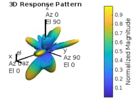
Figure 2. Response pattern of DL pilot decontamination
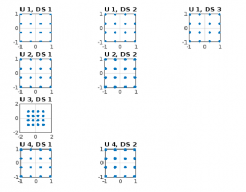
Figure 3. Equalized constellation per stream
The response pattern of the proposed system shows that each of the signaling pattern has the highest magnitude spread of waves shown through Figure 2 and the constellation steam of uplink and downstream in Figure 3.
SINR $=\frac{\text { signalpower }}{\text { noise }+ \text { interferencepower }}$ (39)
Table 1 shows comparative analysis based on the error occurrence for the number of bits transferred with the specified model.
Table 1. Comparative analysis based on error vector magnitude with no. of bits transferred
|
Parameters |
Error Vector Magnitude |
No. of Bits |
|
ROMP |
1.0311 |
3114 |
|
SAMP |
1.0024 |
6234 |
|
Pro_CSLSS |
0.38361 |
9354 |
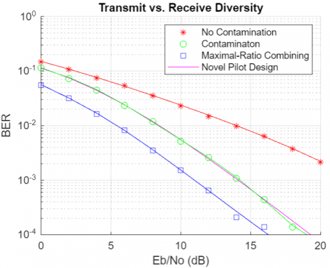
The comparison of various strategies representing their diversity with the receival value divergence. Figure 4 indicates the least divergence for the novel pilot contamination strategy having higher processing of lesser diversity between the transmitted and received signals.
Table 2. Comparative analysis based on compressive sensing between existing and proposed technique
|
Parameters |
ROMP [13] |
SAMP [15] |
Pro_CSLSS |
|
MSE versus SNR |
74.6 |
72.2 |
64.5 |
|
BER versus SNR |
54.9 |
52.8 |
41.2 |
|
Throughput versus the number of antennas in BS |
93.2 |
94 |
97.8 |
|
throughput versus SNR |
92.5 |
96 |
97.5 |
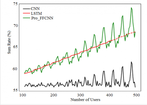
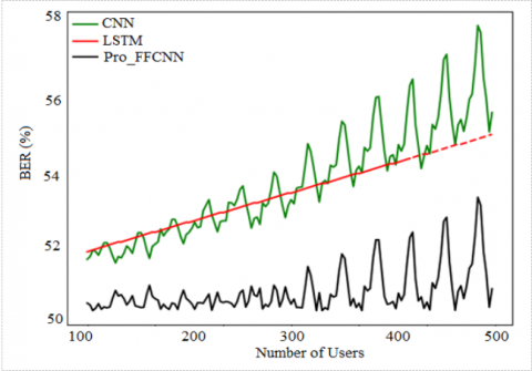
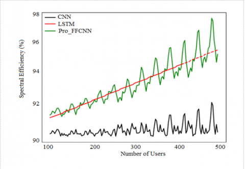
Table 3. Comparative analysis based on interference alignment using deep learning between existing and proposed technique
|
Parameters |
CNN [19] |
LSTM [20] |
Pro_FFCNN |
|
Sum rate versus number of users |
67.6 |
69.5 |
74.6 |
|
BER versus number of users |
53.8 |
54.5 |
57.8 |
|
SINR versus number of users |
75 |
76.8 |
79.8 |
|
Spectral efficiency versus the number of users |
93.5 |
96 |
98 |
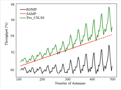
A comparison of the parameters between the existing and new compressive sensing approaches is shown in Table 2. MSE in terms of SNR, BER in terms of SNR, throughput in terms of the number of antennas in BS, and throughput in terms of SNR are the metrics taken into consideration in compressive sensing.
The comparison between the existing and proposed techniques is shown in Table 3 utilizing interference alignment and deep learning. The metrics taken into account for compressive sensing are BER, sum rate, SINR, and spectral efficiency in terms of user count.
Figure 5 comparison of parameter analysis between the proposed and existing compressive sensing techniques with respect to MSE, BER, throughput for the number of antennas, and throughput for SNR.
Figure 6 below illustrates a comparison of the existing and suggested solutions employing interference alignment and deep learning.
Sum rate, BER, SINR, and spectral efficiency in terms of user count are the variables up for comparison when it comes to interference alignment. From above comparative analysis, the proposed FFCNN based interference alignment system obtained optimal results when compared with the existing deep learning techniques. Interference has been aligned and improved sum rate by 74.6%, BER is improved by 57.8%, SINR by 79.8% and spectral efficiency of the channel has been improved by 98% for number of users. Therefore, proposed FFCNN based interference alignment system mitigates the interference of the network by enhancing the above-discussed parameters.
(a) MSE versus SNR
(b) BER versus SNR
(c) Throughput versus the number of antennas in BS
(d) Throughput versus SNR
Figure 5. Comparison of parameter analysis between the proposed and existing compressive sensing techniques; (a) MSE; (b) BER; (c) throughput for no. of antennas; (d) throughput for SNR
(a) Sum rate vs the number of users
(b) BER vs the number of users
(c) SINR vs the number of users
(d) spectral efficiency vs the number of users
Figure 6. Comparative analysis based on interference alignment using deep learning (a) sum rate, (b) BER, (c) SINR, (d) Spectral efficiency
In a large MIMO method, this research provided a novel technique for pilot decontamination and interference alignment-based channel estimation. Here, the goal is to lessen PC attacks by adopting a Compressive Sensing-Based Location Scheduling System (CSLSS) for a user-friendly pilot sequence. The pilot set will be optimised with an additional sequence thanks to our location-based decontamination technique. A feed-forward convolutional neural network is used to do interference alignment in MIMO (FFCNN). The results of the experiment are reviewed, and the parameters used for analysis include BER, sum rate, SINR, and spectral efficiency in terms of interference alignment. Compressive sensing parameters include MSE, BER, throughput versus the number of antennas in BS, and throughput versus SNR. The suggested technique has eliminated pilot contamination based on compressive sensing and interference alignment has been achieved by deep learning technique in channel modelling, according to experimental analysis based on both compressive sensing and deep learning techniques.
We would like to thank to the VFSTR Deemed University, Guntur and BIT Mesra, Ranchi for providing the infrastructure facilities in the Department of ECE to carry on this research work.
[1] Zhang, J.Y., Björnson, E., Matthaiou, M., Ng, D.W.K., Yang, H., Love, D.J. (2020). Prospective multiple antenna technologies for beyond 5G. IEEE Journal on Selected Areas in Communications, 38(8): 1637-1660. https://doi.org/10.1109/JSAC.2020.3000826
[2] Abdulateef, A.A., Ibrahim, S.M., Mohammed, A.H., Abdulateef, I.A. (2020). Performance analyses of channel estimation and precoding for massive MIMO downlink in the TDD system. In 2020 4th International Symposium on Multidisciplinary Studies and Innovative Technologies (ISMSIT), IEEE, pp. 1-6. https://doi.org/10.1109/ISMSIT50672.2020.9255189
[3] Gong, Z.J., Li, C., Jiang, F. (2019). Pilot decontamination in noncooperative massive MIMO cellular networks based on spatial filtering. IEEE Transactions on Wireless Communications, 18(2): 1419-1433. https://doi.org/10.1109/TWC.2019.2892775
[4] Xiong, C.Y., Chen, S.Y., Li, L., Wu, Y.C. (2021). Pilot assignment based on graph coloring and location information in multicell multiuser massive mimo systems. Wireless Communications and Mobile Computing, 2021: 1-12. https://doi.org/10.1155/2021/9913149
[5] Akbar, N., Yan, S.H., Yang, N., Yuan, J.H. (2016). Mitigating pilot contamination through location-aware pilot assignment in massive MIMO networks. In 2016 IEEE Globecom Workshops (GC Wkshps), IEEE, pp. 1-6. https://doi.org/10.1109/GLOCOMW.2016.7848962
[6] Khan, I., Singh, M., Singh, D. (2018). Compressive sensing-based sparsity adaptive channel estimation for 5G massive MIMO systems. Applied Sciences, 8(5): 754. https://doi.org/10.3390/app8050754
[7] Hirose, H., Ohtsuki, T., Gui, G. (2020). Deep learning-based channel estimation for massive MIMO systems with pilot contamination. IEEE Open Journal of Vehicular Technology, 2: 67-77. https://doi.org/10.1109/OJVT.2020.3045470
[8] Abdullah, Q., Abdullah, N., Salh, A., Audah, L., Farah, N., Ugurenver, A., Saif, A. (2021). Pilot contamination elimination for channel estimation with complete knowledge of large-scale fading in downlink massive mimo systems. arXiv Preprint arXiv: 2106.13507. https://doi.org/10.48550/arXiv.2106.13507
[9] Ma, J.P., Zhang, S., Li, H.Y., Zhao, N., Leung, V.C. (2018). Interference-alignment and soft-space-reuse based cooperative transmission for multi-cell massive MIMO networks. IEEE Transactions on Wireless Communications, 17(3): 1907-1922. https://doi.org/10.1109/TWC.2017.2786722
[10] Muppirisetty, L.S., Charalambous, T., Karout, J., Fodor, G., Wymeersch, H. (2018). Location-aided pilot contamination avoidance for massive MIMO systems. IEEE Transactions on Wireless Communications, 17(4): 2662-2674. https://doi.org/10.1109/TWC.2018.2800038
[11] Mohammadghasemi, H., Sabahi, M.F., Forouzan, A.R. (2019). Pilot-decontamination in massive MIMO systems using interference alignment. IEEE Communications Letters, 24(3): 672-675. https://doi.org/10.1109/LCOMM.2019.2959780
[12] de Figueiredo, F.A., Mathilde, F.S., Santos, F.P., Cardoso, F.A., Fraidenraich, G. (2016). On channel estimation for massive MIMO with pilot contamination and multipath fading channels. In 2016 8th IEEE Latin-American Conference on Communications (LATINCOM), IEEE, pp. 1-4. https://doi.org/10.1109/LATINCOM.2016.7811581
[13] Lahbib, N.D., Cherif, M., Hizem, M., Bouallegue, R. (2022). BER analysis and CS-based channel estimation and HPA nonlinearities compensation technique for massive MIMO system. IEEE Access, 10: 27899-27911. https://doi.org/10.1109/ACCESS.2022.3147353
[14] Sheikhi, A., Razavizadeh, S.M., Lee, I. (2020). A comparison of TDD and FDD massive MIMO systems against smart jamming. IEEE Access, 8: 72068-72077. https://doi.org/10.1109/ACCESS.2020.2987606
[15] Ge, L.J., Zhang, Y., Chen, G.J., Tong, J. (2019). Compression-based LMMSE channel estimation with adaptive sparsity for massive MIMO in 5G systems. IEEE Systems Journal, 13(4): 3847-3857. https://doi.org/10.1109/JSYST.2019.2897862
[16] Khan, I., Singh, D. (2018). Efficient compressive sensing based sparse channel estimation for 5G massive MIMO systems. AEU-International Journal of Electronics and Communications, 89: 181-190. https://doi.org/10.1016/j.aeue.2018.03.038
[17] Han, Y., Jin, S., Wen, C.K., Ma, X.L. (2020). Channel estimation for extremely large-scale massive MIMO systems. IEEE Wireless Communications Letters, 9(5): 633-637. https://doi.org/10.1109/LWC.2019.2963877
[18] Al-Salihi, H., Nakhai, M.R. (2017). Efficient Bayesian compressed sensing-based channel estimation techniques for massive MIMO-OFDM systems. EURASIP Journal on Wireless Communications and Networking, 2017(1): 1-10. https://doi.org/10.1186/s13638-016-0796-9
[19] Ramisetty, U.M., Chennupati, S.K., Gundavarapu, V.N.K. (2021). Design of training sequences for multi user-MIMO with accurate channel estimation considering channel reliability under perfect channel state information using cuckoo optimization. Journal of Electrical Engineering & Technology, 16(5): 2743-2756. https://doi.org/10.1007/s42835-021-00778-6
[20] Zhang, Y.S., Xiang, Y., Zhang, L.Y., Rong, Y., Guo, S. (2018). Secure wireless communications based on compressive sensing: A survey. IEEE Communications Surveys & Tutorials, 21(2): 1093-1111. https://doi.org/10.1109/COMST.2018.2878943
[21] Sun, B., Zhou, Y.Q., Yuan, J.H., Shi, J.L. (2020). Interference cancellation based channel estimation for massive MIMO systems with time shifted pilots. IEEE Transactions on Wireless Communications, 19(10): 6826-6843. https://doi.org/10.1109/TWC.2020.3006208
[22] Khwandah, S.A., Cosmas, J.P., Lazaridis, P.I., Zaharis, Z.D., Chochliouros, I.P. (2021). Massive MIMO systems for 5G communications. Wireless Personal Communications, 120(3): 2101-2115. https://doi.org/10.1007/s11277-021-08550-9
[23] Huang, C.W., Alexandropoulos, G.C., Zappone, A., Yuen, C., Debbah, M. (2019). Deep learning for UL/DL channel calibration in generic massive MIMO systems. In ICC 2019-2019 IEEE International Conference on Communications (ICC), IEEE, pp. 1-6. https://doi.org/10.1109/ICC.2019.8761962
[24] DeepMIMO 5G NR. https://deepmimo.net/versions/5gnr/, accessed on 25 May 2023.