Saraswathi Elumalai*![]() | Faritha Banu Jahir Hussain
| Faritha Banu Jahir Hussain![]()
© 2023 IIETA. This article is published by IIETA and is licensed under the CC BY 4.0 license (http://creativecommons.org/licenses/by/4.0/).
OPEN ACCESS
The economic health of a nation is significantly influenced by the productivity of its agricultural sector. Enhancing this productivity is directly linked to the early detection and management of plant diseases. Automated classification methodologies are instrumental in the early diagnosis of these diseases, offering improved precision over traditional methods. These automated systems initiate disease detection as soon as symptoms begin to manifest on plant leaves, following a four-step process involving pre-processing, segmentation, feature extraction, and classification. In this study, we present an automated methodology for the detection and classification of plant diseases using a deep-learning approach applied to varying quality leaf images. A deep convolutional neural network architecture was trained utilizing an image dataset. The proposed Deep Neural Network Plant Disease Classifier (DNN-PDC) was specifically designed for the multi-categorization of plant diseases. Tomato leaf images from the PlantVillage dataset on Kaggle were selected for the experiments. The proposed deep learning system demonstrated a high level of accuracy in the classification of various tomato leaf diseases, including Early Blight, Septoria Leaf Spot, and Late Blight. Experimental results indicate that the proposed method surpasses existing approaches in the image-based classification of tomato plant diseases. This study underscores the potential of the DNN-PDC model as a highly effective tool for plant disease detection and classification.
activation function, convolutional neural network, deep learning, feature extraction, image processing, plant disease classification, PlantVillage dataset, segmentation
Untimely detection of plant diseases can escalate food insecurity, thereby adversely impacting the yield and quality of agricultural products. Consequently, effective disease prevention and control hinge on early detection and forecasting, playing a pivotal role in agricultural production management and decision-making. Traditional methods of plant disease identification largely leaned on visual inspections by field specialists, a process that is labor-intensive, time-consuming, and unsuitable for large-scale applications [1]. Furthermore, real-time and rapid diagnosis of plant diseases remains unachievable with this approach. To assuage these challenges, Wang et al. [2] introduced an innovative approach for plant disease detection, which notably ameliorates classification efficacy while addressing issues linked to agricultural challenges.
Most plant diseases are initially detectable on plant leaves, opening avenues for automated detection through high-quality image processing. However, the task of plant disease detection through image processing is complicated due to considerable differences in leaf color, texture, and shape across different and related plant species. Several researchers have developed a range of data mining-based feature extraction methods in the initial stages, including block-level correlations following the Markov model, discrete wavelet differential clustering models, bags of visual words, and convolutional neural networks [3]. These techniques generate high-dimensional features without requiring human experts, yet the dimensionality of the image emerges as a significant challenge.
The loss of crops can profoundly influence a country's economy, making it critical to diagnose plant diseases promptly and take necessary measures to prevent crop losses. A wide array of diseases plague crops in the temperate, tropical, and subtropical regions of the world. Environmental variables such as rainfall and moisture levels can propagate certain plant diseases caused by various viruses, fungi, bacteria, and other pathogens [4]. These diseases can severely impact farmers' livelihoods. Therefore, early detection of plant diseases is crucial for maintaining crop health, especially as agricultural advancements promise enhancements in both crop yield and quality.
Traditionally, the diagnosis of plant diseases has heavily relied on human expertise, a reality that is not always feasible in remote and underdeveloped areas. Furthermore, traditional methods employed by farmers and field specialists for identifying plant diseases are time-consuming, expensive, and error-prone [5]. Thus, artificial intelligence-based methods can play a significant role in diagnosing plant disease in a rapid and accurate manner. Image processing and data modeling tools have assisted farmers and agricultural experts in identifying diseases. Automated methods for assessing the quality of agricultural and aquaculture products can also analyze images, which are then used to construct a detection model for plant diseases.
Significant strides have been made in applying deep learning techniques to agricultural problems such as insect detection, fruit and leaf disease detection, and plant and leaf categorization [6]. However, executing real-time disease diagnosis with typical machine learning algorithms poses significant challenges. Hence, deep learning methodologies can aid in the development of expert systems in the agricultural industry.
Complex phytopathological issues coupled with the vast variety of crops make it challenging for even agronomists to correctly identify plant diseases. As such, systems employing deep learning and computer vision can aid field specialists and farmers in diagnosing plant diseases by analyzing input images of leaf tissue. These state-of-the-art systems employ a large number of training parameters, necessitating long learning curves and powerful computational resources [7]. This study attempts to reduce the number of features used for prediction while maintaining classification accuracy for detecting plant diseases using the CAE network, significantly reducing training and prediction time.
Deep Learning approaches are modeled on the architecture of the human brain. They use variants like Convolutional and Recurrent Neural Networks to find hidden structures in data. Compared to Machine Learning, Deep Learning has two primary advantages: they extract multiple features from raw data automatically, eliminating the need for an additional feature extraction module, and they can process large datasets with many dimensions in a fraction of the time [8]. Many computer vision applications utilize two Deep Learning techniques, convolutional neural networks (CNNs), and convolutional autoencoders (CAEs) due to their efficacy with image data. Both strategies employ convolution operations to extract various spatial and temporal features from image data, with CAEs being more efficient in reducing the dimensionality of an image than CNNs in classifying input images.
While research and findings are promising, there remains a need to explore the potentials of developing artificial intelligence-based systems using advanced neural network designs with substantial accuracy in the field of plant species recognition and disease detection. To enhance the robustness and efficiency of these automatic classification models, they are modeled on a wide variety of crops from different types and quality settings [8]. The proposed effort in this study aims to develop a plant disease detection and classification system using deep learning. Plant leaves' images from diverse health and disease categories were analyzed. The compiled dataset includes images from databases from various countries, ensuring the proposed framework's global applicability [9-11].
Using both laboratory and field images, the framework is solidified. Multiple rounds of dense convolutional neural network models are trained on a big collection of images from diverse categories. Complex background factors contribute to a wide range of differences between and within classes. Training, validation, and testing sets are created from the collected data for testing and training purposes [12, 13]. The trained architecture is cross-validated five times and tested on unseen images to ensure that it is accurate and efficient. On fivefold cross-validation and other unseen test images, the suggested deep learning-based solution outperformed all previous methods by an accuracy of 96% [14]. For plant health monitoring and early disease diagnosis, the suggested framework has demonstrated good results with actual, fixed-resolution operation and integration [9].
The main contributions of the research conducted and presented in this paper are as follows:
With the advent of smartphones and the expansion of mobile apps, simple and easy-to-use applications may be designed to improve agricultural infrastructure and give information on plant disease identification [15]. Plant and crop monitoring using a live image capturing device to detect Phyto pathological concerns may be done using new prototypes created for use with autonomous agricultural vehicles. Using a mobile or computer application, these devices may be managed and monitored in an easy-to-use framework. The plant disease identification problem may be tackled with the use of image processing techniques and specific statistical characteristics. Mobile devices are used to identify wheat crop candidate hotspots [16].
Deep learning, an advanced form of machine learning, was developed as a result of advancements in the realm of graphics processing units (GPUs) and the availability of technology applications based on cognitive technologies. In contrast to ordinary neural networks, deep learning designs often consist of several layers. Plant disease identification has been aided by a variety of machine learning and deep learning methods [17]. The user-defined characteristics used in basic machine learning algorithms are used to distinguish images from different categories. To identify and classify characteristics, deep learning methods use the architecture's many levels to decide them on their own. Plant diseases including grape leaf disease, potato blight disease, palm oil leaf disease, and others have long been recognized using support vector machines (SVMs) [18].
Sustained learning techniques like SVM are used for data categorization, however, they require custom features in order to distinguish between distinct classes. SVM-trained ANN classifiers having an accuracy of 92.17 percent were used to extract texture and colour characteristics from plant leaves. The categorization of rice blasts, a significant problem, is aided by an enhanced KNN algorithm based on image processing and the k-means approach in Lab colour space. This approach was able to detect rice blasts with a 94% success rate [19]. Plants of black grime are susceptible to chlorosis, commonly known as yellowing sickness.
A support vector machine-based computer vision system for identifying Chlorosis in plant leaves was suggested and achieved a 95.69 percent accuracy rate. Machine learning and other statistical approaches suffer from a lack of performance since they require manual characteristics for their operation [20]. This led to the development of NN-based approaches with a diagnosis of crop diseases in big datasets. The plants of the Vigna were classified as good, moderate, and disease classes by a convolutional neural network. Different pre-processing approaches are used to train the sequential network. The model achieved a 97.403% accuracy value for different images. Transfer learning was utilised to train the EfficientNet architecture with a disease classifier, and numerous images were used for the training process in the experimentation [20, 21].
Disease identification in the alpine grasslands can also be accomplished using hyperspectral imaging techniques [22]. PCA (Principal component analysis), spatial catalogues, range elimination, and spinoffs were all employed in the arduous circumstances of high spatial homogeneity. A total of four machine learning-based techniques generated a 94.73 percent success rate. Bacteriosis, a prevalent disease in peach crops, was detected using an imaging and convolutional neural network technique. Pre-processing leaf images with a variety of adaptive processes, such as channel selection and gray-level slicing, allows for the most accurate results [23]. Bacteriosis detection using a deep learning model has an overall accuracy of 98.75 percent.
Plant diseases and their severity may be detected using a computer network called PD2 SE-Net. Five crops in three distinct groups and Resnet-50 architecture are used as a basic network for training images in different categories [24]. Using transfer learning, a system for detecting disease in the Casava plant was developed and found to be 93% accurate in unseen images. The development of AI (Artificial Intelligence) cleared the path for the creation of robotic machines which could achieve precise findings in disease detection. Today, artificial intelligence-based technologies that can identify a wide range of diseases are widely employed. Traditional machine learning methods have been suggested in the recent decade over disease classification [25].
Various researchers used Support Vector Machines (SVMs) to study the early detection and categorization of diseases in sugar beets (SVM). Using K-means and Artificial Neural Networks (ANN), some researchers were able to identify five different plant leaf diseases. To diagnose six distinct diseases on cotton leaves, some researchers came up with a novel technique. Image processing characteristics such as edges, colours, and textures may all be used to create a feature vector that can be used to pick the best features to use in a Particle Swarm Optimization (PSO)-based feature selection approach to classify disease [26]. In a separate investigation, researches used the SVM approach to identify and detect two distinct viruses that cause disease on tomato leaves [27-35]. In a separate study, some researchers used the Local Binary Pattern approach to identify three distinct vine leaf diseases via SVM. Images processing-based candidate hotspot identification and the Naive Bayes classifier were suggested by some researchers focused on early detection of three wheat illnesses by use of a mobile phone application. They tested a strategy on mobiles with a real-world setting to see if it worked [28].
The logistic algorithm Group Method Data Handling (GMDH) was recently introduced for automated plant disease detection. Classification performance is directly impacted by the difficulty of the feature extraction procedure necessary for machine learning classification. The discovery of novel approaches that can handle real-time data lacking the requirement for unique characteristics cleared the door for deep learning systems [29]. Many layers and neurons in deep neural networks can handle enormous amounts of data effectively to execute high-complexity tasks like speech and image recognition. Deep learning techniques are increasingly being used in the detection and categorization of diseases based on medical imagery [30].
Neural networks-based research identification of disease detection was investigated in a review paper published in 2019 and the possibilities of deep learning were appraised. Instead of identifying entirely disease detection-based dataset, it has been shown that the majority of research utilises the PlantVillage database to identify disease in a single plant or a few crops. In one of these researches, some researchers used Convolutional Neural Networks to classify 13 distinct plant diseases (CNN). A suggested model was trained on 30,880 images, and a test model was tested on 25,89 images, in this work. The accuracy of their proposed model was 96.3 percent on average. Some researchers used the DENS-INCEP deep transfer learning model to find rice plant disease in their study.
VGGNet has been an adapted module that allowed to perform of disease classification on maize and rice plants in a separate investigation. A total of 39 categories in the PlantVillage dataset, comprising five studies identified plant illnesses and a category of ambient images devoid of leaves. Various CNN models were used by researchers to classify plant diseases [31]. They were able to get a classification accuracy of 99.35 percent in their research. VGG16, Brainstorm V4, ResNet50, ResNet101, Resnet152, and Dense Nets 121 are only a few of the CNN models. With fewer parameters and less computation time than other models, the DenseNet architecture utilised in the study was shown to have the best test accuracy of 99.75 percent. With a varied epoch, batch size, and dropout, the researchers designed the 9-layer CNN model on the PlantVillage dataset and compared its performance with popular transfer learning algorithms.
In analysing the given dataset, their suggested model accomplished a classification accuracy of 96.46 percent. On the other side, two other studies have added additional images to the PlantVillage collection [32]. Ferentinos used the test dataset and the neural network architectures to classify 58 distinct plant diseases across 25 different species. With a 99.53 percent accuracy rate, the VGG architecture employed in the study was the most accurate. 79,265 images from the PlantVillage dataset were developed by some researchers in a second research attempt, which used the larger PlantDisease dataset. Both datasets were used in the experiments. Classifying leaves in the second stage of the proposed two-stage PlantDiseaseNet classification model is a key component of this approach [33]. In the Plant Disease dataset, the model they provided had an accuracy rate of 93.67%. Deep learning architectures have also been studied to see how well they classify plant diseases in both PlantVillage and commercial datasets. Image segmentation and image classification phases were included in the model described by some researchers for the identification of plant diseases [34].
In the image segmentation step, they suggested a hybrid segmentation technique based on hue, saturation, intensity, and LAB, and in the classification phase, they employed CNN models. As some colleagues expanded the which was before MobileNetV2 model by adding the Classification Activation Map (CAM), they came up with a new plant disease detection model dubbed MobileNet-Beta. The suggested model was evaluated using data from PlantVillage as well as data from the authors' research. The MobileNet-Beta model was shown to be 99.85 percent accurate, according to the test findings [34].
3.1 Image pre-processing
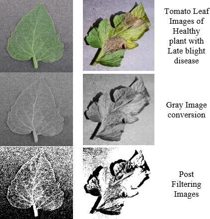
Imperfections in image acquisition, data transmission, and recording devices can produce poor visualizations and computer processing challenges during the image production process, degrading the image quality. There are several elements that can impact image quality such as imaging system noise, environmental conditions, and so on. Before performing any image analysis, it is required to perform images pre-processing such as grey transformation and image denoising. Sample Images in pre-processing stage are shown in Figure 1.
As a result of unequal lighting circumstances and varied times or locations for photography, we may suppose the plant leaf image $I_{x, y}$ is composed of a grey backdrop $G r_{x, y}$, leaf diseases $D_{x, y}$ and background errors $\operatorname{Err}_{x, y}$ in the image. Background images must be removed in order for the bilinear interpolation method to work properly, and this is done by using the grey transformation method. Each block of the image is used as a starting point for determining the image's backdrop colour. Despite the overall image's uneven lighting, it may be regarded as virtually uniform in the immediate vicinity. Using bilinear interpolation, we may create a continuous surface by interpolating four consecutive pixels that are contiguous to each other as part of the image's grey transformation process. So, the image can be represented as:
$I_{x, y}=G r_{x, y}+D_{x, y}+E r r_{x, y}$ (1)
Some noise in the image can be caused by external influences, which might have a detrimental effect on feature extraction. Consequently, image denoising is required, with traditional filtering algorithms like median filtering as well as Gaussian filtering being employed because of their widespread use and the fact that they are right and superior in certain issues over time. Using the predetermined median, a central template pixel's grey value is altered using the median filtering technique. The median of all the template pixels is calculated. Despite being less sensitive to noise and doing a better job of reducing salt and pepper noise, this approach may easily break up an image.
Using a gradient inverted weighted approach, the image edges and details are blurred while noise is suppressed, thus the median technique is compared on this basis. While the grayscale transformation in a region is smaller than the grayscale changes between regions, there is a greater difference in their absolute values. This can be seen in a $m \times m$ window by looking at how much each neighbour point's weight differs depending on where it is located in relation to the region's centre pixel, which has a larger weight value than the neighbour points on the periphery and outside of the area. It is therefore possible to use a weighted average instead of an arithmetic one to improve the algorithm and avoid blurring its boundaries.
When applying filters or convolutions to an image, such as blurring or smoothing filters, a common operation involves computing the average of neighbouring pixel values. In the case of an arithmetic average, all pixels within the filter's neighbourhood contribute equally to the computed value. This can result in blurring or smoothing across edges, as the intensity values on both sides of an edge are averaged together. In this approach, the weights are determined based on the distance from the center pixel or the application of edge detection algorithms to identify and assign higher weights to pixels along edges. By incorporating a weighted average, our algorithm can effectively balance the smoothing or blurring effect across an image while preserving important edge information. This can result in improved boundary delineation, sharper image features, and better overall image quality for tasks that require edge preservation or edge-aware processing.
Figure 1. Sample images in pre-processing stage
So, with these preliminaries, we are estimating the gradient inverse(h) based on the gray value as:
$h(x, y, m, n)=\frac{1}{g(x+m, y+m)-g(x, y)}$ (2)
$\forall m, n=-1$ or 0 or 1 and $m \neq n \neq 0$ (3)
The neighbourhood pixel gradient inverse(S) is estimated and we get the weight matrix in normalised form as:
$\begin{gathered}s={\left[\begin{array}{ccc}s(x-1, y-1) & s(x-1, y) & s(x-1, y+1) \\ s(x, y-1) & s(x, y) & s(x, y+1) \\ s(x+1, y-1) & s(x+1, y) & s(x+1, y+1)\end{array}\right]}\end{gathered}$ (4)
Assuming that the total of the weights of the eight other points is equal to 1, the centre point is given a weight of 0.5. The weight may therefore be calculated for each location as:
$S(x+m, y+n)=\frac{1}{2} \frac{h(x, y, m, n)}{\sum_m \sum_n h(x, y, m, n)}$ (5)
Grayscale conversion from colour images is a typical image processing technique. It's true that grayscale images don't convey as much information as colour ones, yet there are times when it's useful or even vital. In contrast to colour pictures, which use three different channels (red, green, and blue), grayscale images only use one (intensity). This simplification makes it less difficult to conduct specific operations on the picture by decreasing the computational complexity, memory requirements, and processing time.
3.2 Image segmentation
One of the most important techniques for analyzing and comprehending images is segmentation, which breaks an image into non-overlapping sections. Leaf image segmentation is used to differentiate diseased sections of leaves from healthy ones, resulting in a binary image that may be used for feature extraction and computation. For this reason, a unique grey threshold must be determined for each image because the colors of different varieties of leaves aren't identical. A large variation $(\delta)$ can be seen between the grey levels in various places, yet the grey levels within the same region are frequently identical. There is a high grey level difference $\left(\rho_C^2\right)$ between two sections separated by threshold u. If the difference in the average grey of the two regions is greater than that of the overall average grey of the image. This feature may be expressed using the regional grey variance, which has the following formula.
$\alpha_C^2=\rho_1(u)\left[\delta_1(u)-\delta\right]^2+\rho_2(u)\left[\delta_2(u)-\delta\right]^2$ (6)
$\delta=\delta_1(u) \gamma_1(u)+\delta_2(u) \gamma_2(u)$ (7)
$\rho_C^2=\delta_1(u) \delta_2(u)\left[\delta_1(u)-\delta_2(u)\right]^2$ (8)
where, $\alpha_C^2$ represents variance between two segmented regions in order to estimate the threshold t. It is important to identify when the variance between two segmented sections reaches its highest value as a result of this study, the threshold for binarizing the image might be the normalized grey value.
Finding a suitable threshold for image segmentation can be a challenging task, especially when manual selection or exhaustive calculation is not practical. The image is divided into smaller regions, and the threshold is determined for each region individually. Common adaptive thresholding techniques include mean thresholding, Gaussian thresholding, and median thresholding. In this approach, Gaussian thresholding is used, which is found to be suitable for thresholding.
3.3 Feature extraction
Image analysis is frequently concerned with an image's distinctive features and specifics. During recognition and classification, the image characteristics could be produced and extracted by separating usable information from non-useful information; this allowed for additional computation to be done. Automatic image identification or evaluation can be achieved by extracting relevant signs from images using a technique known as image feature extraction. Image identification and classification rely heavily on feature extraction, which directly impacts model quality. Many elements may be retrieved from leaf images, including geometric features, textures, and colours.
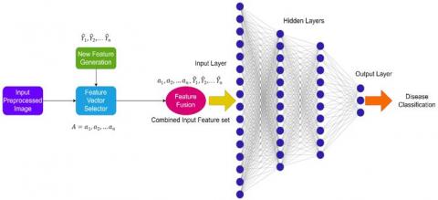
This work focuses on extracting the leaf images' features from the aforementioned aspects, such as geometric features, textures, and colours. Normal and sick leaves have highly distinct textures because of their various thicknesses and directions of the repeating patterns and rules that make up an image's texture. The grey scale may thus be used to quantify the disease spots' properties of roughness, sharpness, and texture. Because the grey-level co-occurrence matrix of an image contains all of the information needed to statistically define texture properties, it is frequently used as a starting point for analysing images. For example, HSI mode is more compatible with the human eye's perception of colour, and it can separate colour features first from the brightness information of an image, making it easier for a computer to modify the recognition pattern based on varied lighting conditions. An overview of Deep Learning model for multi-class classifiers is depicted in Figure 2.
Figure 2. Overview of deep learning model for multi-class classifier
However, because a single colour space may only hold so much information about a disease's symptoms, the HSI, as well as RGB properties, are combined to create a more complete colour space. The severity of the disease may be gauged by looking at the size and form of the disease spots on the leaves, which vary in size and shape depending on the disease severity. Spots are merely a reflection of the disease's form aspects, and it is not important to examine the leaf disease's colour. In this case, the grayscale images of leaves may be converted to binary images, which simplifies the process while also reducing the amount of storage required. The binary image is labelled with 0 or 1 depending on the value of the grayscale. The following are the features extracted for our proposed work:
1. $C=\sum_{m, n=0 S m n}|m-n|^2$ that determines the contrast value(C) and estimated from the co-occurrence matrix entries $S(m, n)$.
2. $E=\sum S(m, n)^2$ defines the energy(E) estimated by summing up all the elements by squaring them and ranges between 0 and 1.
3. $\operatorname{cor}=\sum_{m, n} \frac{\left(m-\mu_m\right)\left(n-\mu_n\right) s(m, n)}{\sigma_m \sigma_n}$ provides the correlation value(cor) that falls between -1 and 1.
4. $H=\frac{S(m, n)}{1+|m-n|}$ gives the homogeneity value (H) derived between 0 and 1.
While converting a grayscale image into a binary image during feature extraction, it typically involves applying a thresholding operation to separate the image into foreground and background regions. The resulting binary image contains only two intensity values, typically represented as black and white pixels, indicating the presence or absence of objects or features. Once the binary image is obtained, a feature extraction technique can be applied to analyze and describe the characteristics of the objects or regions present in the image. These extracted features capture important information about the shape, texture, size, or spatial distribution of objects, which can be useful for subsequent analysis, classification, or recognition tasks. These features can then be used for decision-making processes in leaf disease detection.
Multi-class data feature selection is a difficult process. The majority of known feature selection methods are based on binary datasets. Methods for selecting the most important characteristics from a huge number of features can be found by using the well-known area under the ROC (AUC) curve. Binary classification issues are commonly analysed using AUC. Multi-class AUC is used in this article to identify the most important characteristics for categorising the dataset. Multi-class AUC is briefly discussed here using an example of a multi-class situation to illustrate the point.
3.4 Dataset
The leaves of different crops are categorized into distinct groups. Using the input layer of the deep learning architecture, the images used in the proposed work were translated from several datasets with varying resolutions into the same dimensions. It is necessary to create a good dataset before dividing the acquired information into training, validation, and testing sets. A deep learning architecture is then taught utilising this data in numerous epochs. A variety of criteria are used to gauge the model's overall performance. Unseen images belonging to all categories were also examined by the trained model following 5-fold cross-validation. Models are trained and tested on a specific dataset in order to produce a competent leaf classification and the disease diagnosis procedure. The four datasets each contain a separate set of images, one for each type of damaged or healthy plant.
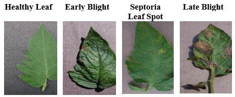
More than 25,000 images of plant leaves were gathered from the PlantVillage collection. These leaf images are from three different crops, including Apples, Potatoes, and Tomatoes. A total of 17 distinct levels are available. Only three classes of leaf images from each crop were classified as healthy, while the others were classified as unhealthy. We have chosen Tomato leaves images from the dataset and trained the model. The various combination of images with healthy tomato leaves, and the leaves affected with the diseases such as Early blight, Septoria leaf spot, and Late blight.
In the dataset, the number of tomato leaf images is up to 18,060. Out of which, 6,748 images were taken for the proposed work. The following details in Table 1 shows different categories and images.
Table 1. Categories of tomato leaf in PlantVillage dataset
|
S.No. |
Category |
Number of Images |
|
1. |
Bacterial Spot |
2027 |
|
2. |
Early bilght |
1000 |
|
3. |
Late bilght |
1909 |
|
4. |
Mold leaf |
952 |
|
5. |
Septoria Leaf spot |
1771 |
|
6. |
Spider mites |
1676 |
|
7. |
Target spot |
1404 |
|
8. |
Tomato mosaic virus |
373 |
|
9. |
Tomato yellow curl virus |
5357 |
|
10. |
Healthy |
1591 |
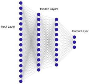
In the field of computer vision and image categorization, deep learning has had a significant impact. There are a variety of layers in deep convolutional neural networks, such as convolutional layers, pooling layers, and fully connected layers with various activation functions. The convolutional neural network's input layer transforms the incoming data to fit its specific dimensions. An object's classification is learned and differentiated from other sorts of objects by processing the incoming data layer by layer. It is believed that training a deep convolutional neural network will be faster, more accurate, and deeper if the connectivity between layers between input and output is kept as short as feasible. The proposed Deep Learning process has been explained with the diagram as shown in Figure 3.
Figure 3. Proposed deep learning process
Convolutional neural networks have a feed-forward connection structure, with each layer feeding information to the next. Traditional n-layer convolutional neural networks have $n$ connections between each layer, one for each succeeding layer in the network. However, with dense convolution, there are $\frac{n(n+1)}{2}$ direct connections. All previous layers' feature maps are utilised as inputs into the current layer, while the current layer's feature maps are used as inputs into the next layer. The first layer receives input and generates $\mathrm{k}$ feature maps, which are then combined with the input data. Additional $m$ set of feature maps is generated using the second layer, which is then combined with the first. This results in $m \times n$ feature maps being generated for each $N$ layered dense block. Table 2 shows the CNN layer structure.
Table 2. CNN layer structure
|
Layers |
Output Size |
Architecture |
|
Convolution |
112*112 |
Convolution |
|
Pooling |
56*56 |
MaxPool |
|
Dense Block 1 |
56*56 |
Convolution |
|
Transition Layer |
28*28 |
AveragePool |
|
Dense Block 2 |
14*14 |
Convolution |
|
Classification Layer |
3*1 |
SoftMax |
|
DNN-PDC Multi Class Classifier Algorithm |
||
|
Input: Pre-processed Leaf images Output: Classification into a Disease Class Steps: 1. Estimate the Feature score of the multiclass dataset. 2. Let Feature set $A=a_1, a_2, \ldots a_n$ and the disease classes as $B \in \mathbf{1}, 2,3$. 3. For any combination of $\left\{a_i, B\right\}$: a. Set threshold $\theta$ based on the ROC value of feature vectors. b. Generate corresponding n feature score values and compare with $\theta$. c. Create a new feature set with features $\boldsymbol{a}_i$ such that $a_i>\theta$. 4. For an $n$-dimensional feature vector from step 3, Calculate the output vector $\widehat{\boldsymbol{Y}}=\emptyset\left(\sum_{j=1}^n \boldsymbol{a}_j \boldsymbol{w}_j+\right.$ bias $)$, where $\boldsymbol{w}_j$ denotes weight value for the neuron. 5. Estimate connection weights by the backpropagation algorithm. 6. Compute error as $e r r=\frac{1}{2} \sum_{j=1}^n(Y-\widehat{Y})^2$. 7. Back propagate the error term err and adjust neuron weight in the hidden layer as: $w_{i j}^{\text {updated }}=w_{i j}^{\text {original }}-\rho \tau \widehat{Y}^y$ for the $y^{t h}$ hidden layer with the learning parameter $(\boldsymbol{\rho})$ $\mathbf{0} \leq \rho \leq 1$. 8. Estimate $(\boldsymbol{\tau})$ $\tau=\left\{\begin{array}{c}\text { err } \times \widehat{Y}, \text { For Output Layer nodes } \\ \widehat{Y} \sum_{i, j=1, y=1}^n \rho_y w_{i j}, \text { For hidden Layer nodes }\end{array}\right.$ 9. Train the model with newly identified features $a$ with the identified disease class labels. 10. Combine the feature sets $a_1, a_2, \ldots a_n$ and $\widehat{Y}_1, \widehat{Y}_2, \ldots \widehat{Y}_n$. 11. Input the new pre-processed image to check the classifier performance and accuracy. |
As opposed to other models, such as ResNet, AlexNet, and so on, the model has improved the precision of CNN architectures with a small number of attributes. Traditional convolutional neural networks have a lot more parameters than dense connection patterns, but they don't have to learn duplicate feature maps. There are several tiers in DenseNet201, and it has performed well. As the name implies, DenseNet is "dense", meaning that every layer is interconnected with every other layer. Architectures based on feature reuse and gradient flow are also advantageous. The compact network makes it simple to train the DenseNet201. There is a lot of variances in the succeeding layers' input because of the feature reuse functionality employed by various levels in order to improve speed.
Furthermore, DenseNet outperformed other deep learning architectures while using fewer parameters. A greater amount of information may be gleaned from dense networks than from simpler networks. This training deep learning compact model uses 224×224-pixel images of plant leaves as input. 16 output channels in DenseNet are utilised to convolution an input image that is supplied to the dense blocks. Each dense block has a direct feedforward connection between all the levels in the block. Each layer's feature maps are analysed individually and combined into a single tensor before being sent to the next layer. The activation function used is the Rectifier Linear Unit (ReLU) because of its computing efficiency. Batch normalisation and convolutions of three-by-three are also used to feature maps.
As a result of batch normalisation, a transition layer is added between the dense blocks, which are made up of convolutions of 1:1 and pooling averages of 2:2. One further layer of global average pooling connects the final dense block before a softmax classifier is added. After that, classification is performed on all of the previously taught labels, and a plant leaf image is tested using a similar technique. Several convolutional layers and dense blocks are used to process the plant leaf image. Predicted images in a given category are determined using block-by-block processing once a model has been trained. The first two layers of a fully connected layer utilise a dropout approach to prevent overfitting in deep learning architectures by randomly blocking particular neurons based on a preset probability value. Diseases alter the leaf's appearance by infecting it, and the resulting patterns can be used as visual cues by a machine learning system. Different patterns created by disease and the morphology of the leaf images are used to identify infected and healthy images in a deep learning network.
Deeper architectures allow for hierarchical feature extraction, capturing both low-level and high-level features. The increased capacity enables the model to capture more intricate relationships within the data, potentially improving accuracy. In this approach, Non-linear activation functions, such as ReLU (Rectified Linear Unit), introduce non-linearity into the neural network, enabling it to learn more complex and expressive representations. Non-linear activation functions can help the network model intricate decision boundaries and improve accuracy compared to linear activation functions. Also,used regularization techniques L1 regularization prevents overfitting, which occurs when a model becomes too specialized to the training data and performs poorly on unseen data. Regularization techniques encourage the model to generalize better and can improve accuracy.
GPU support was employed to compile all models in this investigation. An NVIDIA Tesla K80 with 12GB of memory and a 64-bit Debian GNU/Linux 9.11 operating system were used for all experimental tests in the Google cloud environment. Everything is developed in Python using the Keras 2.3.1 framework, an open-source deep neural network toolkit. A total of 90% of the original and augmented PlantVillage datasets were randomly divided into training and validation sets while 3% of the total datasets were randomly separated into test and validation sets. When building the model, the training and validation datasets were used only for that purpose, whereas the test set was used to determine how well the model predicted the outcomes of samples it had never seen before. The transfer learning strategy was employed in conjunction with already existing CNN models in this study.
Figure 4. Training and validation loss analysis
Pre-trained CNN models on the ImageNet dataset allowed us to quickly discover and categorise all of the categories in the dataset. It is estimated that the ImageNet database has 1.2 million photos grouped into 1,000 different classifications. For the deep learning models utilised in this work, pre-trained weights from the most recent generation of CNN models on ImageNet were employed to save training time. There were 39 outputs added to all models with 1000 outputs in response to the issue. All the layers of pre-trained models were set to be trainable. For the last layer, we used Softmax to activate the function and category cross entropy for the loss function. The early halting strategy was utilised with patience as 5 and a minimum change in loss as 1e-3 throughout training. Training and validation loss analysis has been shown in Figure 4.
Table 3. Performance comparison
|
Model |
Training Accuracy |
Training Loss |
Testing Accuracy |
Testing Loss |
|
DenseNet 201 |
99.9 |
0.02487 |
89.56 |
0.08954 |
|
EfficientNet B5 |
98.85 |
0.03458 |
91.35 |
0.12547 |
|
DNN-PDC |
99.94 |
0.002549 |
94.68 |
0.00324 |
The maximum epoch for training models was not determined because the early halting strategy was employed. It utilised the same optimization strategy that was used for ImageNet training. All other models are optimised using Adam, whereas the VGG16 model is optimised using SGD. There is a notable difference between the Adam and SGD methods when it comes to their learning rates. All models have their validation step set to one. After normalising each pixel value in the original and supplemented datasets, the results were compared. After that, the photos were downsized to fit the specifications of each model, which varied widely. Table 3 shows the performance comparison among various neural models.
Table 4. Model trainnig parameters
|
S. No. |
Training Parameters |
Values |
|
1. |
Learning Rate |
0.01 |
|
2. |
Batch Size |
128 |
|
3. |
Number of Epochs |
100 |
|
4. |
Optimizer |
Adam |
|
5. |
Loss Function |
cross-entropy loss |
Table 4 shows the training parameters of the model.Because of the constraints of our technology, we had to reduce the input image resolution for all models of EfficientNet architecture. 132*132 was found to be the greatest input size for which our hardware resources could train the model with the most parameters in the trial-and-error research. 132*132 has been chosen as the input size so that all models of EfficientNet architecture may be evaluated under the same circumstances. During backpropagation, weights and biases are updated using a mini-batch of data. In most cases, a value that can be divided by the total number of samples in the dataset is desirable for the mini-batch value. Network convergence and accurate prediction may be improved with the help of this value. Different parameters of the Neural Network model have been listed in Table 5.
Table 5. Neural network model parameters
|
Model Name |
Image Size |
Optimization Method |
Learning Rate |
|
DenseNet 201 |
113*113 |
Adam |
0.001 |
|
EfficientNet B5 |
132*132 |
Adam |
0.001 |
|
DNN-PDC |
132*132 |
Adam |
0.01 |
Figure 5. Confusion matrix
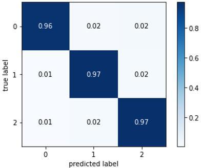
All models' hardware resources permitted a maximum mini-batch size of 16, hence that was the value used in this investigation. PlantVillage's dataset has 39 different categories, hence a multi-class classification algorithm was used to sort the data. False Positive (FP) and False Negative (FN) indices are used to create metrics based on the confusion matrix values acquired in such classifications (FN). For example, in this example, TP refers to the number of correctly classified diseased photos in each category, whereas TN indicates the total number of correctly categorised images in all other categories except for the relevant category. A number of photos that have been incorrectly categorised. Except for the appropriate category, FP displays the total number of images that were incorrectly categorised. In Figure 5, the confusion matrix for the proposed approach has been shown.
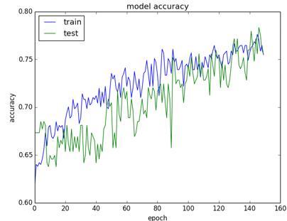
Figure 6. Proposed model training and testing accuracy analysis
Different measures, including Accuracy (A), Sensitivity (Sy), Specificity (Sp), and Precision (P) are used to evaluate EfficientNet's and other cutting-edge CNN models (P). Sensitivity is the percentage of true positives that are accurately anticipated. The ratio of accurately predicted negatives to all genuine negatives measures the degree of specificity. On the other hand, accuracy measures the percentage of samples that are properly categorised. Precision is the percentage of positive identifications that are accurately anticipated. EfficientNet deep learning architecture's performance in classifying plant leaf disease will be evaluated, and the results will be compared with those of other, more advanced CNN models that have been previously published. These models were all trained by transferring knowledge from one model to another. Figure 6 shows the proposed model training and testing accuracy analysis.
$S y=\frac{T P}{T P+F N}$
$S p=\frac{T N}{T N+F p}$
$A=\frac{T P+T N}{T P+F N+T N+F P}$
$P=\frac{T P}{T P+F P}$
All experiments were conducted using both original and enhanced datasets. It is important to note that in this context the average of the test dataset accuracy, sensitivity, specificity, and precision values achieved by all models on the test dataset. For training purposes, the period from when loss values began to rise to when they stopped was considered to be the entire training time. The entire training time was divided by the total number of epochs, and the result was presented as the time spent per epoch during model training. There was a lot of overlap between the models' average accuracy scores in the original dataset The EfficientNet model has the best average sensitivity across all classes in the original dataset. Sample Images from PlantVillage are shown in Figure 7.
Figure 7. Sample images from PlantVillage
In contrast, the average performance of models in predicting other classes was near to each other. The EfficientNet model's true positive classification rate (precision) was greater than the other models' true positive classification rate (precision). While the EfficientNet model took over years to complete a single epoch, the training took just 643.3 minutes. EfficientNet obtained the lowest training time per epoch. Using the ratio of properly identified samples to the total sample count, these test accuracy numbers were derived. In the original dataset, the EfficientNet model had 99.91 percent accuracy, whereas the proposed model had 99.97 percent accuracy in the enhanced dataset. Additionally, EfficientNet accuracy scores were 99.45% for the original datasets and 99.67% for the enhanced datasets, the lowest of any model. It is clear from the test accuracy curves that all models perform better on the enhanced dataset than on the original. The proposed model training and testing loss analysis has been depicted in Figure 8.
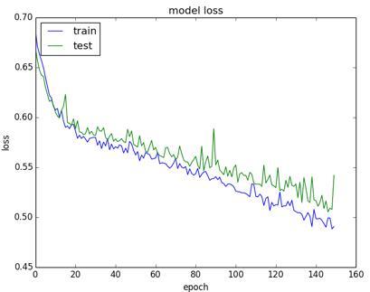
Figure 8. Proposed model training vs testing loss analysis
In the original and enhanced datasets, the EfficientNet and proposed models' results for the TP, TN, FP, FN, accuracy, sensitivity, specificity, and precision are summarised. EfficientNet obtained the greatest performance in the original dataset with a precision of 84.75 percent to 100 percent, whereas DNN-PDC earned a precision of 96.08 percent to 100 percent in the supplemented dataset with a precision of 96.28% to 100 percent It was found that for each class, the EfficientNet model achieved an accuracy rate between 99.54 and 100% in the original dataset whereas the DNN-PDC model achieved an accuracy rate of between 99.85 and 100% in the supplemented dataset while examining the test datasets for accuracy. For the EfficientNet and DNN-PDC models, the validation loss began to rise around the 20th and 11th epochs, respectively, due to the early halting approach utilised in training. Precision-Recall curve for the proposed approach has been depicted in Figure 9.
Figure 9. Precision-recall curve for the proposed approach
These models were tested on training sets and validation sets to see how well they performed on both. This dataset had an accuracy of 98 percent after just six iterations, and it reached its peak accuracy after 20 epochs of training. Loss in the enhanced dataset was minimised greatly after 11 iterations and its best accuracy was obtained at over 98% at that point. EfficientNet and DNN-PDC models scored the greatest accuracy and precision scores in the test dataset compared to other deep learning models, with 99.91 percent and 99.97 percent for accuracy and 98.42 percent and 99.39 percent for precision, respectively.
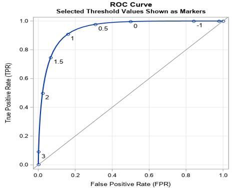
Figure 10. FPR vs TPR curve
Figure 10 shows the ROC curve obtained for the proposed approach. A tight range of 99.45 to 99.97 percent accuracy was observed in the models, while the precision metric showed that the accuracy values fluctuated more significantly between 90.26 percent and 99.39 percent. When the rate of false positives drops, so does precision, which measures how many out of every 100 samples the model predicts will be positive. The DNN-PDC model, which performed best on the expanded dataset, improved accuracy, and precision by 0.13 percent and 2.16 percent, respectively, while all other models improved accuracy and precision by varying degrees. It was clear from this that as the volume of data grew, so did the precision of the models' false-positive predictions. The prediction accuracy analysis has been depicted in Figure 11.
Figure 11. Prediction accuracy analysis
In this paper, we have proposed a deep learning model (DNN-PDC) for the classification of diseases of the Tomato plant leaves. The proposed approach has four stages such as pre-processing, segmentation, extraction of features, and classification. We have chosen tomato leaf images of the PlantVillage dataset from Kaggle for the experiments. The suggested deep learning-based system was found to be capable of accurately classifying a wide range of tomato leaf diseases such as Early blight, Septoria leaf spot, and Late blight. The proposed DNN-PDC model has been compared with the existing DenseNet 201 and EfficientNet B5 to analyse the performance of the existing approaches. From the experimental results, we can conclude that the proposed approach outperforms the existing approaches in the classification of disease of the tomato plant from the images. As an extension of this work, in the future, for achieving better performance than the proposed one, a self-organizing network structure can be created by applying a highly optimal layer-wise propagation strategy to data linkages specified within the related graph structure.
[1] Keceli, A. S., Kaya, A., Catal, C., Tekinerdogan, B. (2022). Deep learning-based multi-task prediction system for plant disease and species detection. Ecological Informatics, 69: 101679. https://doi.org/10.1016/j.ecoinf.2022.101679
[2] Wang, K., Chen, K., Du, H., Liu, S., Xu, J., Zhao, J., Liu, Y. (2022). New image dataset and new negative sample judgment method for crop pest recognition based on deep learning models. Ecological Informatics, 69: 101620. https://doi.org/10.1016/j.ecoinf.2022.101620
[3] Yang, C.K., Lee, C.Y., Wang, H.S., Huang, S.C., Liang, P.I., Chen, J.S., Chen, T.D. (2022). Glomerular disease classification and lesion identification by machine learning. Biomedical Journal, 45(4): 675-685. https://doi.org/10.1016/j.bj.2021.08.011
[4] Khan, A.I., Quadri, S.M.K., Banday, S., Shah, J.L. (2022). Deep diagnosis: A real-time apple leaf disease detection system based on deep learning. Computers and Electronics in Agriculture, 198: 107093. https://doi.org/10.1016/j.compag.2022.107093
[5] Shammi, S., Sohel, F., Diepeveen, D., Zander, S., Jones, M.G. (2022). A survey of image-based computational learning techniques for frost detection in plants. Information Processing in Agriculture, 10(2): 164-191. https://doi.org/10.1016/j.inpa.2022.02.003
[6] Pane, C., Manganiello, G., Nicastro, N., Ortenzi, L., Pallottino, F., Cardi, T., Costa, C. (2021). Machine learning applied to canopy hyperspectral image data to support biological control of soil-borne fungal diseases in baby leaf vegetables. Biological Control, 164: 104784. https://doi.org/10.1016/j.biocontrol.2021.104784
[7] Zenhausern, R., Day, A.S., Safavinia, B., Han, S., Rudy, P.E., Won, Y.W., Yoon, J.Y. (2022). Natural killer cell detection, quantification, and subpopulation identification on paper microfluidic cell chromatography using smartphone-based machine learning classification. Biosensors and Bioelectronics, 200: 113916. https://doi.org/10.1016/j.bios.2021.113916
[8] Zheng, Z., Zhang, C. (2022). Electronic noses based on metal oxide semiconductor sensors for detecting crop diseases and insect pests. Computers and Electronics in Agriculture, 197: 106988. https://doi.org/10.1016/j.compag.2022.106988
[9] Zhang, Z., Khanal, S., Raudenbush, A., Tilmon, K., Stewart, C. (2022). Assessing the efficacy of machine learning techniques to characterize soybean defoliation from unmanned aerial vehicles. Computers and Electronics in Agriculture, 193: 106682. https://doi.org/10.1016/j.compag.2021.106682
[10] Jiang, F., Lu, Y., Chen, Y., Cai, D., Li, G. (2020). Image recognition of four rice leaf diseases based on deep learning and support vector machine. Computers and Electronics in Agriculture, 179: 105824. https://doi.org/10.1016/j.compag.2020.105824
[11] Abinaya, S., Devi, M.K. (2022). Enhancing crop productivity through autoencoder-based disease detection and context-aware remedy recommendation system. Application of Machine Learning in Agriculture, pp. 239-262. https://doi.org/10.1016/B978-0-323-90550-3.00014-X
[12] Saravanan, T.M., Karthiha, K., Kavinkumar, R., Gokul, S., Mishra, J.P. (2022). A novel machine learning scheme for face mask detection using pretrained convolutional neural network. Materials Today: Proceedings, 58: 150-156. https://doi.org/10.1016/j.matpr.2022.01.165
[13] Neelakantan, P. (2021). Analyzing the best machine learning algorithm for plant disease classification. Materials Today Proceedings, 2214-7853.
[14] Ip, R.H., Ang, L.M., Seng, K.P., Broster, J.C., Pratley, J.E. (2018). Big data and machine learning for crop protection. Computers and Electronics in Agriculture, 151: 376-383. https://doi.org/10.1016/j.compag.2018.06.008
[15] Chlingaryan, A., Sukkarieh, S., Whelan, B. (2018). Machine learning approaches for crop yield prediction and nitrogen status estimation in precision agriculture: A review. Computers and Electronics in Agriculture, 151: 61-69. https://doi.org/10.1016/j.compag.2018.05.012
[16] Kumar, M., Kumar, A., Palaparthy, V.S. (2020). Soil sensors-based prediction system for plant diseases using exploratory data analysis and machine learning. IEEE Sensors Journal, 21(16): 17455-17468. https://doi.org/10.1109/JSEN.2020.3046295
[17] Saggi, M.K., Jain, S. (2022). A survey towards decision support system on smart irrigation scheduling using machine learning approaches. Archives of Computational Methods in Engineering, 29(6): 4455-4478. https://doi.org/10.1007/s11831-022-09746-3
[18] Ai, Y., Sun, C., Tie, J., Cai, X. (2020). Research on recognition model of crop diseases and insect pests based on deep learning in harsh environments. IEEE Access, 8: 171686-171693. https://doi.org/10.1109/ACCESS.2020.3025325
[19] Sharma, A., Jain, A., Gupta, P., Chowdary, V. (2020). Machine learning applications for precision agriculture: A comprehensive review. IEEE Access, 9: 4843-4873. https://doi.org/10.1109/ACCESS.2020.3048415
[20] Goluguri, N.R.R., Suganya Devi, K., Vadaparthi, N. (2021). Image classifiers and image deep learning classifiers evolved in detection of Oryza sativa diseases: Survey. Artificial Intelligence Review, 54: 359-396. https://doi.org/10.1007/s10462-020-09849-y
[21] Janarthan, S., Thuseethan, S., Rajasegarar, S., Lyu, Q., Zheng, Y., Yearwood, J. (2020). Deep metric learning based citrus disease classification with sparse data. IEEE Access, 8: 162588-162600. https://doi.org/10.1109/ACCESS.2020.3021487
[22] Liu, L., Xie, C., Wang, R., Yang, P., Sudirman, S., Zhang, J., Wang, F. (2020). Deep learning based automatic multiclass wild pest monitoring approach using hybrid global and local activated features. IEEE Transactions on Industrial Informatics, 17(11): 7589-7598. https://doi.org/10.1109/TII.2020.2995208
[23] Rajpal, N. (2020). Black rot disease detection in grape plant (Vitis vinifera) using colour based segmentation & machine learning. In 2020 2nd international conference on advances in computing, communication control and networking (ICACCCN), Greater Noida, India. pp. 976-979. https://doi.org/10.1109/ICACCCN51052.2020.9362812
[24] Bouguettaya, A., Zarzour, H., Kechida, A., Taberkit, A.M. (2022). Deep learning techniques to classify agricultural crops through UAV imagery: A review. Neural Computing and Applications, 34(12): 9511-9536. https://doi.org/10.1007/s00521-022-07104-9
[25] Albattah, W., Nawaz, M., Javed, A., Masood, M., Albahli, S. (2022). A novel deep learning method for detection and classification of plant diseases. Complex & Intelligent Systems, 8: 507-524. https://doi.org/10.1007/s40747-021-00536-1
[26] Perales Gómez, Á.L., López-de-Teruel, P.E., Ruiz, A., García-Mateos, G., Bernabé García, G., García Clemente, F.J. (2022). FARMIT: Continuous assessment of crop quality using machine learning and deep learning techniques for IoT-based smart farming. Cluster Computing, 25(3): 2163-2178. https://doi.org/10.1007/s10586-021-03489-9
[27] Saraswathi, E., FarithaBanu, J. (2023). A novel ensemble classification model for plant disease detection based on leaf images. In 2023 International Conference on Artificial Intelligence and Knowledge Discovery in Concurrent Engineering (ICECONF), Chennai, India, pp. 1-7. https://doi.org/10.1109/ICECONF57129.2023.10083902
[28] Liu, Z., Bashir, R.N., Iqbal, S., Shahid, M.M.A., Tausif, M., Umer, Q. (2022). Internet of Things (IoT) and machine learning model of plant disease prediction-blister blight for tea plant. IEEE Access, 10: 44934-44944. https://doi.org/10.1109/ACCESS.2022.3169147
[29] Khan, S., Tufail, M., Khan, M.T., Khan, Z.A., Anwar, S. (2021). Deep learning-based identification system of weeds and crops in strawberry and pea fields for a precision agriculture sprayer. Precision Agriculture, 22(6): 1711-1727. https://doi.org/10.1007/s11119-021-09808-9
[30] Nieuwenhuizen, A.T., Tang, L., Hofstee, J.W., Müller, J., Van Henten, E.J. (2007). Colour based detection of volunteer potatoes as weeds in sugar beet fields using machine vision. Precision Agriculture, 8: 267-278. https://doi.org/10.1007/s11119-007-9044-y
[31] Umamageswari, A., Deepa, S., Raja, K. (2022). An enhanced approach for leaf disease identification and classification using deep learning techniques. Measurement: Sensors, 24: 100568. https://doi.org/10.1016/j.measen.2022.100568
[32] Gill, T., Gill, S.K., Saini, D.K., Chopra, Y., de Koff, J.P., Sandhu, K.S. (2022). A comprehensive review of high throughput phenotyping and machine learning for plant stress phenotyping. Phenomics, 2(3): 156-183. https://doi.org/10.1007/s43657-022-00048-z
[33] Tee, C.A.T., Teoh, Y.X., Yee, L., Tan, B.C., Lai, K.W. (2021). Discovering the Ganoderma boninense detection methods using machine learning: A review of manual, laboratory, and remote approaches. IEEE Access, 9: 105776-105787. https://doi.org/10.1109/ACCESS.2021.3098307
[34] Gopalakrishnan, C., Iyapparaja, M. (2021). Multilevel thresholding based follicle detection and classification of polycystic ovary syndrome from the ultrasound images using machine learning. International Journal of System Assurance Engineering and Management, 1-8. https://doi.org/10.1007/s13198-021-01203-x
[35] Saleem, M.H., Potgieter, J., Arif, K.M. (2021). Automation in agriculture by machine and deep learning techniques: A review of recent developments. Precision Agriculture, 22: 2053-2091. https://doi.org/10.1007/s11119-021-09806-x