Shuhua Xu![]() | Mingming Qi
| Mingming Qi![]() | Xianming Wang
| Xianming Wang![]() | Yilin Dong
| Yilin Dong![]() | Zhongyi Hu
| Zhongyi Hu![]() | Hanli Zhao∗
| Hanli Zhao∗![]()
© 2023 IIETA. This article is published by IIETA and is licensed under the CC BY 4.0 license (http://creativecommons.org/licenses/by/4.0/).
OPEN ACCESS
Owing to the ill-posed problem of image restoration, how to find an effective method to obtain image prior information is still challenging. The total generalized variational model has been successfully applied to image denoising and/or deblurring. However, the high-order gradient of the image is described by using L1 norm in the traditional total generalized variational denoising and deblurring model, which can not effectively describe the local group sparse priors of the image gradient. As a result, the traditional total generalized variational model has some limitations in the ability to suppress the staircase artifacts. In order to solve this problem, one new model is proposed to restore images corrupted by Cauchy noise and/or blur in our paper, where the non-convex data fidelity term is combined with two regularization terms: group sparse representation prior and multi-directional total generalized variation. We use group sparse representation prior information to obtain the nonlocal self-similarity information of similar image block for preserving the details and texture features of the discontinuous or uneven region of the image. At the same time, the noise is fully removed in the uniform region, which improves the image visual quality. Moreover, the gradient information in multiple directions is calculated by the multi-directional total generalized variation regularization term, which can better preserve the edge information of the image. The model is divided into several sub-problems by split Bregman iteration, and each sub-problem is solved efficiently. The experimental results show that this model is superior to other existing models both in terms of visual quality and some image quality evaluation.
image restoration, Cauchy noise, group sparse representation, dictionary learning, multidirectional total generalized variation
Image restoration aims to estimate the original clear image based on an observed image. Cauchy noise [1, 2] is a prevalent impulse noise with the characteristic of a thick tail, which is widely present in radar imaging, astronomical images, biomedical images, and wireless communication systems. Numerous studies have been conducted to remove Cauchy noise, particularly in the wavelet domain. Zhao et al. [3] employed the maximum a posteriori (MAP) estimation of double tree complex wavelet transform for image noise removal. Hill et al. [4] proposed a new method of single-variable shrinkage in the DWT domain, using translation invariant wavelet decomposition for image denoising. Wu et al. [5] utilized a multi-level wavelet convolution neural network to train the denoiser, maintaining more detailed texture during the denoising process and better balancing the size of the receptive field with the computational load.
Recently, variational models based on total variation regularization have been extensively employed for image denoising. Sciacchitano et al. [1] introduced a total variation model [6] for denoising Cauchy noise in images. Mei et al. [2] applied a specialized multiplier alternating direction method [7] to solve the nonconvex total variation minimization problem. However, total variation is influenced by the staircase effect in smooth regions and cannot effectively recover the details and textures of an image, resulting in an oversmoothed image. To address the edge staircase effect, Yang et al. [8] incorporated higher-order total variation to reduce the staircase effect. Parrisoto et al. [9] introduced a high-order anisotropic total variation regularization term that retains and enhances the inherent anisotropy characteristics of an image, recovering the details and textures as much as possible. Shi et al. [10] proposed a nonlinear diffusion equation for denoising to better recover image detail features, including a diffusion coefficient based on gray scale to estimate noise amplitude and a gradient-based diffusion coefficient to control anisotropic diffusion in accordance with the local structure of an image. Liu and Gao [11] proposed a non-blind image deblurring method that combines multi-directional fractional total variation with traditional total variation, addressing the staircase effect and texture loss issues of total variation while effectively preserving texture and edge information.
For images containing not only flat regions but also inclined ones, the total generalized variation (TGV) model demonstrates strong denoising capabilities in single-image denoising. Bredies et al. [12] suggested using total generalized variation as a penalty function for modeling images with edges and smooth changes, exhibiting excellent denoising performance in single-image denoising. Lv [13] proposed a multilook M for total generalized variation-based multiplicative noise removal to eliminate speckle noise from images. Shi et al. [14] introduced a total generalized variation method for reconstructing electrical impedance tomography (EIT), combining the first and second derivative terms as regularizers to address issues related to Tikhonov regularization's excessive smoothness in image reconstruction and the staircase effect in total variation regularization reconstruction. To improve the denoising effect, Zhong et al. [15] presented a high-order TGV regularization variational model based on the automatic selection of spatial adaptive regularization parameters according to local image characteristics. To better restore image texture in a certain direction, Kongskov et al. [16] proposed a texture direction estimation algorithm and a novel direction total generalized variation model (DTGV), which significantly improves texture preservation and noise removal. Li et al. [17] introduced a weighted model of second-order total generalized variation for Gaussian noise removal by incorporating an edge indicator function into the regularizer of the second-order total generalized variation model [12]. To enhance the intensity of the diffusion tensor and improve the image's visual quality, the method employs first and second derivatives. Since the Shearlet transform can sparsely represent an image and generate the best approximation [18], Lv [19] combined the Shearlet transform with a second-order total generalized variation regularization term, proposing a new recovery model for images corrupted with Cauchy noise. Liu [20] developed a hybrid regularization model for image denoising and deblurring by combining the advantages of total generalized variation with the wavelet method. Zhu et al. [21] presented a second-order TGV and wavelet framework-based hybrid regularization method, inheriting the benefits of wavelet framework regularization and second-order TGV. This model not only removes the staircase effect but also preserves sharp edges while maintaining strong sparse estimation capabilities for piecewise smooth functions.
However, since the TGV model processes pixels independently, it disregards the similarity of processed images, resulting in weak robustness against high-amplitude noise. To address this issue, Zhang et al. [22] employed the nonlocal total generalized variation method for image repair and super-resolution reconstruction. To exploit the sparse representation of image block information, Jung and Kang [23] proposed a nonlocal total generalized variation model based on sparse representation, which improves the denoising performance by considering image block similarity. Zhang et al. [24] proposed a nonlocal total generalized variation model based on local similarity, which takes into account the similarity of image patches in the local area and addresses the over-smoothness issue in flat regions. Chen et al. [25] introduced the sparsity based on overlapping group in TGV model, which can improve the denoising effect of TGV by using structural similarity, and the robustness of TGV to strong noise pollution by using the first and second-order gradient information of domain difference.
Compared with the traditional method using local features, the recent variation method using nonlocal information of image has a great improvement of noise removal effect. Ding et al. [26] used the nonlocal self-similarity of natural images to treat a group of similar blocks as an approximate low rank matrix, and expressed the denoising problem of each group as a low rank matrix restoration problem. Laus et al. [27] used a nonlocal, completely unsupervised method to remove the Cauchy noise in the image. Kim et al. [28] used the weighted kernel norm as the regularization term, and used the similar blocks in the image to remove the additive Cauchy noise through nonlocal similarity.
Although the nonlocal method makes use of the similarity among image blocks to improve the denoising effect, the low similarity or dissimilarity among image blocks limits the applicability of the method. In order to overcome these limitations and better consider the structure of the processed image, group or structured sparse representation has been widely studied in the field of image restoration in recent years [29, 30]. The methods based on group or structured sparse representation can capture the internal characteristics of image structure, enhance the inherent local sparsity and nonlocal self-similarity of image, and improve the effect of image deblurring [30-32], image inpainting [33-35], and denoising [36].
Inspired by the fact that group sparse representation could further suppress the staircase effect of the traditional total generalized variational model and multidirectional total generalized variation can better protect the edge structure features of the image and further suppress false edges, we propose a new model to remove noise and/or blur in the image corrupted by Cauchy noise and/or blur. The model uses the prior knowledge of group sparse representation learned from dictionary and higher-order derivative based on nonlocal multi-directional total generalized variation. The prior of group sparse representation can effectively denoise the uniform region and preserve the texture and detail in formation of the image, while the nonlocal multi-directional total generalized variation based high-order derivative prior can denoise the smooth region and preserve the edge in formation of the image. In addition, an effective iterative algorithm is proposed to solve the model.
In this study, a new nonlocal total generalized variation (NLTGV) model for Cauchy noise removal that combines the advantages of total generalized variation and nonlocal means is proposed. The model effectively removes Cauchy noise while preserving image details and textures. The main contributions of this study are as follows:
The rest of this paper is organized as follows: Section 2 describes the proposed NLTGV model and the corresponding optimization algorithm. Section 3 presents experimental results and comparisons with other denoising methods. Finally, Section 4 concludes the paper and discusses future work.
This section briefly introduces the concepts of image restoration based on total variation, group sparse representation model, and total variation model based on overlapping group sparse for image restoration.
2.1 Image restoration based on total variation
The mathematical description of image restoration from an image contaminated with Cauchy noise is given by:
$y=Hx+\eta ,$ (1)
where, x represents an unknown original clear image, y denotes an observed image corrupted by noise, H expresses the degradation or blur operator, and n stands for the Cauchy noise. In other words, η represents a random variable that follows the Cauchy distribution, and its probability density function is:
$P(\eta )=\frac{\gamma }{\pi \left( {{\gamma }^{2}}+{{\left( \eta -\delta \right)}^{2}} \right)},$ (2)
where, γ>0 is a scale parameter that determines the noisy level, and $\delta \in \mathbb{R}$ is a location parameter, which determines the peak's position and is usually set to zero. Since H is irreversible, recovering the clear image x from y is an ill-posed problem.
The model for image restoration from an image contaminated with Cauchy noise includes a total variation regularization term [6] and a nonconvex data-fitting term derived from the probability density function in Eq. (2), as follows:
$\underset{x}{\mathop{\min }}\,\frac{\lambda }{2}<\log \left( {{\gamma }^{2}}+{{\left( Hx-y \right)}^{2}} \right),1>+TV(x).$ (3)
2.2 Group sparse representation model
Traditional sparse representation considers an image block as a sparse representation unit. Assuming an image with size $x \in \mathbb{R}^{\mathrm{N}}$ with size $\sqrt{N} \times \sqrt{N}$ is divided into $m$ image blocks $x_i \in \mathbb{R}^P(i=1,2, \cdots, m)$ with $\sqrt{P} \times \sqrt{P}$ size in step s. Extracting image blocks from an image can be described by the following formula:
${{x}_{i}}={{R}_{i}}(x),$ (4)
where, Ri(⋅)represents the operator to extract the image block, and $R_i^T(\cdot)$ represents the transpose operation of Ri(⋅) to return the image block to the original position of the image. For each image block xi and the given dictionary Di, image block xi can be sparsely represented by Di, as follows:
${{x}_{i}}\text{=}{{D}_{i}}{{\alpha }_{i}},$ (5)
where, αi is the sparse coding coefficient of xi under Di. The whole image recovered from the image blocks can be described by the following formula:
$x\text{=}{{\left( \sum\limits_{i=1}^{m}{R_{i}^{T}{{R}_{i}}} \right)}^{-1}}\sum\limits_{i=1}^{m}{\text{R}_{_{i}}^{T}({{x}_{i}})}\text{=}{{\left( \sum\limits_{i=1}^{m}{R_{i}^{T}{{R}_{i}}} \right)}^{-1}}\sum\limits_{i=1}^{m}{\text{R}_{_{i}}^{T}({{D}_{i}}{{\alpha }_{i}})}.$ (6)
Since the traditional sparse representation does not consider the similarity among image blocks, the group sparse representation model [29] was proposed, which takes the group consisting of image blocks as the unit of sparse representation. Following the study [37], the most similar h-1 image blocks with image block $x_i$ are found in a search window, and the $\mathrm{h}$ image blocks constitute a matrix $x_{G_i}=\left[x_{G_i, 1}, x_{G_i, 2}, \cdots, x_{G_i, h}\right] \in \mathbb{R}^{P \times h}$ by pulling each image block into a column. For each group $x_{G_i}(i=1,2, \cdots, n)$ and a given dictionary $D_{G_i}$, group $x_{G_i}$ consisting of image blocks can be sparsely represented by $D_{G_i}$, as follows:
${{x}_{{{G}_{i}}}}\text{=}{{\text{D}}_{{{G}_{i}}}}{{\alpha }_{{{G}_{i}}}},$ (7)
where, $\alpha_{G_i}$ is the sparse coding coefficient of $x_{G_i}$ under $D_{G_i}$. The whole image recovered from all groups can be described by the following formula:
$\begin{align} & x\text{=}{{\left( \sum\limits_{i=1}^{n}{R_{{{G}_{i}}}^{T}{{R}_{{{G}_{i}}}}} \right)}^{-1}}\sum\limits_{i=1}^{n}{\text{R}_{{{G}_{i}}}^{T}({{x}_{{{G}_{i}}}})} \\ & \text{=}{{\left( \sum\limits_{i=1}^{n}{R_{{{G}_{i}}}^{T}{{R}_{{{G}_{i}}}}} \right)}^{-1}}\sum\limits_{i=1}^{n}{\text{R}_{{{G}_{i}}}^{T}({{D}_{{{G}_{i}}}}{{\alpha }_{{{G}_{i}}}})}, \\\end{align}$ (8)
where, $R_{G_i}(\cdot)$ is the operator of extracting a group, and $R_{G_i}^T(\cdot)$ is the transpose operation of $R_{G_i}(\cdot)$, which returns a group to the original position in the image. $R_{G_i}(\cdot)$ and $R_{G_i}^T(\cdot)$ have the same meaning in the following equations unless stated otherwise.
The image restoration model for restoring x from y based on group sparse representation [29, 38] is as follows:
$\begin{align} & \underset{\left\{ {{\text{a}}_{{{G}_{i}}}} \right\},\{{{D}_{{{G}_{i}}}}\},x}{\mathop{\min }}\,\frac{\lambda }{2}\left\| y-x \right\|_{2}^{2} \\ & +\sum\limits_{i=1}^{n}{\left( {{\mu }_{{{G}_{i}}}}{{\left\| {{\alpha }_{{{G}_{i}}}} \right\|}_{0}}+\left\| {{D}_{{{G}_{i}}}}{{\alpha }_{{{G}_{i}}}}-{{R}_{{{G}_{i}}}}(x) \right\|_{2}^{2} \right)}, \\\end{align}$ (9)
where, $n$ represents the number of image block groups, $D_{G_i}$ denotes the dictionary, and $\alpha_{G_i}$ is the coefficient of sparse coding of image block group $x_{G_i}$ under dictionary $D_{G_i}$.
2.3 Total variation model based on overlapping group sparse
Liu et al. [39] defined the $K \times K$-point group of vector $\mathrm{x} \in \mathbb{R}^{\mathrm{N}}$ stacked by $\sqrt{N} \times \sqrt{N}$ matrix in columns:
$\tilde{x}_{i, j, K}=\left[\begin{array}{cccc}x_{i-m_1, j-m_1} & x_{i-m_1, j-m_1+1} & \cdots & x_{i-m_1, j+m_2} \\ x_{i-m_1+1, j-m_1} & x_{i-m_1+1, j-m_1+1} & \cdots & x_{i-m_1+1, j+m_2} \\ \vdots & \vdots & \ddots & \vdots \\ x_{i+m_2, j-m_1} & x_{i+m_2, j-m_1+1} & \cdots & x_{i+m_2, j+m_2}\end{array}\right] \in \mathbb{R}^{K \times K}$, (10)
where, $m_1=\left[\frac{K-1}{2}\right], m_2=\left[\frac{K}{2}\right],[K], x_{i, j, K}$ is obtained by stacking $\tilde{x}_{i, j, K} \in \mathbb{R}^{K \times K}$ in column order, that is, $x_{i, j, K}=$ $\tilde{x}_{i, j, K}(:)$, the sparse regularization term based on overlapping group [39] is defined as:
$\phi (x)=\sum\limits_{i,j=1}^{\sqrt{N}}{{{\left\| {{x}_{i,j,K}} \right\|}_{2}}}.$ (11)
The size of the group in Eq. (11) is K×K.
The overlapping group sparse total variation (OGS-TV) model [39] is defined as:
$\text{OGS}-\text{TV}(x)=\phi ({{\nabla }_{1}}x)+\phi ({{\nabla }_{2}}x),$ (12)
where, ∇1x and ∇2x represent the first-order gradients of x in the horizontal and vertical directions, respectively.
It is assumed that the Cauchy noise $\eta$ in Eq. (1) follows the Cauchy distribution $C(0, \gamma)$ with the location parameter set to $\delta=0$. In order to restore the unknown original image $\mathrm{x}$, the maximum a posteriori (MAP) estimation is commonly employed by maximizing the conditional posterior probability $p(x \mid y)$. Based on the Bayesian principle $p(x \mid y)=\frac{p(y \mid x) p(x)}{p(y)}$ and the application of negative logarithm operation, the MAP estimation $\mathrm{x}$ is obtained through the minimization of $-\log (p(y \mid x))-\log (p(x))$, which $-\log (p(y \mid x))$ serves as a data-fitting term, while $-\log (p(y \mid x))$ also being utilized as a regularizer. It is further assumed that an observed image $y \in \mathbb{R}^{\sqrt{N}\times \sqrt{N}} $ and its corresponding unknown original image $x \in \mathbb{R}^{\sqrt{N} \times \sqrt{N}}$ are transformed into column vectors according to the matrix columns, indexed by $A=\{1,2, \cdots, \sqrt{N}\} \times\{1,2, \cdots, \sqrt{N}\}$. Given that image pixels are considered independent and identically distributed, there are $p(x)=\prod_{j \in A} p\left(x_j\right)$. The relationship between $\delta=0$ and $p(y \mid x)=p(\eta)$ is established, resulting in $p\left(y_j \mid x_j\right)=\frac{\gamma}{\pi\left(\gamma^2+\left((H x)_j-y_j\right)^2\right)}$. By taking logarithms on both sides of this relationship, the following equation is derived:
$\begin{aligned} & -\log (\mathrm{p}(\mathrm{y} \mid \mathrm{x}))=-\sum_{\mathrm{j} \in \mathrm{A}} \log \left(\mathrm{p}\left(\mathrm{y}_{\mathrm{j}} \mid \mathrm{x}_{\mathrm{j}}\right)\right) \\ & =\sum_{\mathrm{j} \in \mathrm{A}} \log \left(\gamma^2+\left((\mathrm{Hx})_{\mathrm{j}}-\mathrm{y}_{\mathrm{j}}\right)^2\right)+\log \pi-\log \gamma .\end{aligned}$ (13)
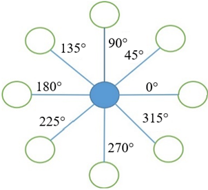
As discussed in Section 2.2, the nonlocal self-similarity of the image is leveraged, and a more robust geometric structure is preserved through the prior knowledge of group sparse representation. Consequently, the data fidelity term is combined with group sparse representation in the model for Cauchy noise removal. In order to further preserve edge information in multiple directions of an image, the multi-directional total generalized variation method introduces two additional diagonal directions, as depicted in Figure 1, in accordance with the traditional directional total generalized variation model. This allows for the detection of edge features in eight distinct directions during image restoration. In conjunction with overlapping group sparsity [39], the overlapping group sparse multidirectional total generalized variation (MDTGV) regularization term is defined as follows:
$\text{MDTGV}(x)=\underset{w}{\mathop{\min }}\,\left\{ {{\lambda }_{1}}\sum\limits_{j=1}^{4}{\begin{align} & \phi \left( {{\nabla }_{j}}x-{{w}_{j}} \right) \\ & +{{\lambda }_{0}}\sum\limits_{j=1}^{16}{\phi \left( {{\left[ \varepsilon \left( w \right) \right]}_{j}} \right)} \\\end{align}} \right\},$ (14)
where, $\nabla_1 x$ and $\nabla_2 x$ are described in Section 2.3, $\nabla_3 x$ and $\nabla_4 x$ represent the first-order gradients of $x$ in the diagonal $45^{\circ}$ and $135^{\circ}$ directions, respectively, and $\varepsilon(w)_j=\nabla_j w_j+\sum_{i=1 \text { and } i \neq j}^4 \frac{\nabla_i}{2} w_j(j=\{1,2,3,4\})$ denotes the second-order gradient operator.
Figure 1. Eight domain space of pixels
Building upon the overlapping group sparse multidirectional total generalized variation model, a method for eliminating Cauchy noise from an image is proposed as follows:
$\begin{align} & \underset{x,\text{w}}{\mathop{\min }}\,\frac{\lambda }{2}<\log \left( {{\gamma }^{2}}+{{\left( Hx-y \right)}^{2}} \right), \\ & 1>+{{\lambda }_{1}}\sum\limits_{j=1}^{4}{\phi \left( {{\nabla }_{j}}x-{{w}_{j}} \right)+{{\lambda }_{0}}\sum\limits_{j=1}^{16}{\phi \left( {{\left[ \varepsilon \left( w \right) \right]}_{j}} \right)}}. \\\end{align}$ (15)
In summary, two types of priors are combined: group sparse representation priors (GSR) and overlapping group sparse multidirectional total generalized variation (MDTGV). Thus, a new model for denoising images contaminated with Cauchy noise and/or blur is proposed in this study:
$\begin{align} & \underset{\{{{a}_{{{G}_{i}}}}\},\{{{D}_{{{G}_{i}}}}\},\{{{x}_{{{G}_{i}}}}\},\text{w}}{\mathop{\min }}\,\sum\limits_{i=1}^{n}{\left( \frac{\lambda }{2}<\log \left( {{\gamma }^{2}}+{{\left( H{{x}_{{{G}_{i}}}}-{{y}_{{{G}_{i}}}} \right)}^{2}} \right),\text{ }1>+{{\mu }_{{{G}_{i}}}}{{\left\| {{\alpha }_{{{G}_{i}}}} \right\|}_{0}}+\left\| {{D}_{{{G}_{i}}}}{{\alpha }_{{{G}_{i}}}}-{{x}_{{{G}_{i}}}} \right\|_{2}^{2}+{{\lambda }_{1}}\sum\limits_{j=1}^{4}{\phi \left( {{\nabla }_{j}}{{x}_{{{G}_{i}}}}-{{w}_{j}} \right)+{{\lambda }_{0}}\sum\limits_{j=1}^{16}{\phi \left( {{[\varepsilon \left( w \right)]}_{\text{j}}} \right)}} \right)}, \\ & \\\end{align}$ (16)
where, $x \in \mathbb{R}^{\sqrt{N} \times \sqrt{N}}, y \in \mathbb{R}^{\sqrt{N} \times \sqrt{N}}, D_{G_i} \in \mathbb{R}^{P \times k}(P<<k), \alpha_{G_i} \in \mathbb{R}^{k \times h}, x_{G_i} \in \mathbb{R}^{P \times h}$, and $\mathrm{n}$ represent the number of image block groups, as described in subsection 2.2. The regularization parameters $\lambda_1$ and $\lambda_0$ are utilized to balance the first-order difference and the second-order difference in multidirectional total generalized variation.
3.1 Decomposition of model (16)
The model (16) proposed in this study is non-convex due to data fidelity terms and the product of $D_{G_i}$ and $\alpha_{G_i}$. Auxiliary variables $p \in \mathbb{R}^N, q_j \in\left(\mathbb{R}^{P h}\right)^2(j=\{1,2,3,4\}), r_j \in\left(\mathbb{R}^{\mathrm{Ph}}\right)^4(j=\{1,2, \cdots, 16\})$ and $z \in \mathbb{R}^N$ are introduced, allowing the unconstrained model (16) to be rewritten as:
$\begin{align} & \underset{\{{{a}_{{{G}_{i}}}}\},\{{{D}_{{{G}_{i}}}}\},\{{{x}_{{{G}_{i}}}}\},\text{w,p,q,r,z}}{\mathop{\min }}\,\sum\limits_{i=1}^{n}{\left( \frac{\lambda }{2}<\log \left( {{\gamma }^{2}}+{{\left( z-{{y}_{{{G}_{i}}}} \right)}^{2}} \right),\text{ }1>+{{\mu }_{{{G}_{i}}}}{{\left\| {{\alpha }_{{{G}_{i}}}} \right\|}_{0}}+\left\| {{D}_{{{G}_{i}}}}{{\alpha }_{{{G}_{i}}}}-p \right\|_{2}^{2}+{{\lambda }_{1}}\sum\limits_{j=1}^{4}{\phi \left( {{q}_{j}} \right)+{{\lambda }_{0}}\sum\limits_{j=1}^{16}{\phi \left( {{r}_{j}} \right)}} \right)}, \\ & s.t. z=H{{x}_{{{G}_{i}}}},p={{x}_{{{G}_{i}}}},{{q}_{j}}={{\nabla }_{j}}{{x}_{{{G}_{i}}}}-{{w}_{j}},{{r}_{j}}=\varepsilon {{(w)}_{j}}. \\\end{align}$ (17)
By incorporating a penalty term into the constraint condition, the constrained model (17) is relaxed to the following unconstrained model:
$\underset{\{{{a}_{{{G}_{i}}}}\},\{{{D}_{{{G}_{i}}}}\},\{{{x}_{{{G}_{i}}}}\},\text{w,p,q,r,z}}{\mathop{\min }}\,\;\;\sum\limits_{i=1}^{n}{\left\{ \begin{align} & \frac{\lambda }{2}<\log \left( {{\gamma }^{2}}+{{\left( z-{{y}_{{{G}_{i}}}} \right)}^{2}} \right),\text{ }1>+{{\mu }_{{{G}_{i}}}}{{\left\| {{\alpha }_{{{G}_{i}}}} \right\|}_{0}}+\left\| {{D}_{{{G}_{i}}}}{{\alpha }_{{{G}_{i}}}}-p \right\|_{2}^{2}\text{+}{{\lambda }_{1}}\sum\limits_{j=1}^{4}{\phi \left( {{q}_{j}} \right)+}{{\lambda }_{0}}\sum\limits_{j=1}^{16}{\phi \left( {{r}_{j}} \right)} \\ & +\frac{{{\Upsilon }_{1}}}{2}\sum\limits_{j=1}^{4}{\left\| {{q}_{j}}\text{-(}{{\nabla }_{j}}{{x}_{{{G}_{i}}}}-{{w}_{j}}) \right\|_{2}^{2}\text{+}\frac{{{\Upsilon }_{2}}}{2}\sum\limits_{j=1}^{16}{\left\| {{r}_{j}}-\varepsilon {{(w)}_{j}} \right\|_{2}^{2}+\frac{\beta }{2}\left\| p\text{-}{{x}_{{{G}_{i}}}} \right\|_{2}^{2}+\frac{\xi }{2}\left\| z-H{{x}_{{{G}_{i}}}} \right\|_{2}^{2}}} \\\end{align} \right\}},$ (18)
where, $\beta, \Upsilon_1, \Upsilon_2$ and $\xi$ are parameters greater than 0 . In order to solve the model (18), an alternating minimization algorithm (AMA) [38] is employed, which minimizes one variable while keeping other variables fixed and iterates this process. When AMA is applied to model (18), the following subproblems arise:
$({{a}_{{{G}_{i}}}},{{D}_{{{G}_{i}}}})\in \underset{{{a}_{{{G}_{i}}}},{{D}_{{{G}_{i}}}}}{\mathop{\arg \min }}\,{{\mu }_{{{G}_{i}}}}{{\left\| {{\alpha }_{{{G}_{i}}}} \right\|}_{0}}+\left\| {{D}_{{{G}_{i}}}}{{\alpha }_{{{G}_{i}}}}-p \right\|_{2}^{2},$ (19)
$p\in \underset{p}{\mathop{\arg \min }}\,\left\| {{D}_{{{G}_{i}}}}{{\alpha }_{{{G}_{i}}}}-p \right\|_{2}^{2}+\frac{\beta }{2}\left\| p\text{-}{{x}_{{{G}_{i}}}} \right\|_{2}^{2},$ (20)
$q\in \underset{q}{\mathop{\arg \min }}\,{{\lambda }_{1}}\sum\limits_{j=1}^{4}{\phi \left( {{q}_{j}} \right)}\text{+}\frac{{{\Upsilon }_{1}}}{2}\sum\limits_{j=1}^{4}{\left\| {{q}_{j}}\text{-(}{{\nabla }_{j}}{{x}_{{{G}_{i}}}}-{{w}_{j}}) \right\|_{2}^{2}},$ (21)
$r\in \underset{r}{\mathop{\arg \min }}\,{{\lambda }_{0}}\sum\limits_{j=1}^{16}{\phi \left( {{r}_{j}} \right)}\text{+}\frac{{{\Upsilon }_{2}}}{2}\sum\limits_{j=1}^{16}{\left\| {{r}_{j}}-\varepsilon {{(w)}_{j}} \right\|_{2}^{2}},$ (22)
$\begin{align} & z\in \underset{z}{\mathop{\arg \min }}\,\frac{\lambda }{2}<\log \left( {{\gamma }^{2}}+{{\left( z-{{y}_{{{G}_{i}}}} \right)}^{2}} \right), \\ & \text{ }1>\text{+}\frac{\xi }{2}\left\| z-H{{x}_{{{G}_{i}}}} \right\|_{2}^{2}, \\\end{align}$ (23)
$\begin{align} & {{x}_{{{G}_{i}}}}\in \underset{{{x}_{{{G}_{i}}}}}{\mathop{\arg \min }}\,\frac{\beta }{2}\left\| p\text{-}{{x}_{{{G}_{i}}}} \right\|_{2}^{2}\text{+}\frac{{{\Upsilon }_{1}}}{2}\sum\limits_{j=1}^{4}{\left\| {{q}_{j}}\text{-(}{{\nabla }_{j}}{{x}_{{{G}_{i}}}}-{{w}_{j}}) \right\|_{2}^{2}} \\ & \text{+}\frac{\xi }{2}\left\| z-H{{x}_{{{G}_{i}}}} \right\|_{2}^{2}, \\\end{align}$ (24)
$\begin{align} & w\in \underset{w}{\mathop{\arg \min }}\,\frac{{{\Upsilon }_{1}}}{2}\sum\limits_{j=1}^{4}{\left\| {{q}_{j}}\text{-(}{{\nabla }_{j}}{{x}_{{{G}_{i}}}}-{{w}_{j}}) \right\|_{2}^{2}} \\ & \text{+}\frac{{{\Upsilon }_{2}}}{2}\sum\limits_{j=1}^{16}{\left\| {{r}_{j}}-\varepsilon {{(w)}_{j}} \right\|_{2}^{2}}. \\\end{align}$ (25)
3.2 Solving $\left(a_{G_i}, D_{G_i}\right)$ sub-problems
With $\mathrm{p}$ fixed, the subproblem (19) for $\left(a_{G_i}, D_{G_i}\right)$ is resolved. By fixing $D_{G_i}$ and $p$, the minimization problem of $a_{G_i}$ becomes:
$\underset{{{a}_{{{G}_{i}}}}}{\mathop{\min }}\,{{\mu }_{{{G}_{i}}}}{{\left\| {{\alpha }_{{{G}_{i}}}} \right\|}_{0}}+\left\| {{\text{D}}_{{{G}_{i}}}}{{\alpha }_{{{G}_{i}}}}-p \right\|_{2}^{2}.$ (26)
The Orthogonal Matching Pursuit (OMP) algorithm [40] can be utilized to solve the subproblem (26). OMP, an iterative greedy algorithm, selects the most relevant column to the current residuals in $D_{G_i}$ at each step. The OMP algorithm stops when the error $\left\|D_{G_i} \alpha_{G_i}-p\right\|_2^2$ falls below $\theta^2$ ( $\theta$ is a very small number). In order to obtain the dictionary $D_{G_i}$, the KSVD algorithm [41] is employed to solve the subproblem (19). In fact, the sparse coding and dictionary are repeatedly updated $\mathrm{J}$ times within the KSVD algorithm.
3.3 Solving p and z subproblems
The subproblem of solving $\mathrm{p}$ in (20) is a least square problem. Assuming $L=\min _p\left\|D_{G_i} \alpha_{G_i}-p\right\|_2^2+$ $\frac{\beta}{2}\left\|p-x_{G_i}\right\|_2^2$, the partial derivatives of $\mathrm{p}$ for $\mathrm{L}$ is $\frac{\partial L}{\partial p}=2\left(p-D_{G_i} a_{G_i}\right)+\beta\left(p-x_{G_i}\right)$, and letting $\frac{\partial L}{\partial p}=0$, the closed-form solution of the $p$ subproblem in (20) is as follows:
$p\text{=}{{\left( 2I+\beta I \right)}^{-1}}\left( 2{{D}_{{{G}_{i}}}}{{a}_{{{G}_{i}}}}+\beta {{x}_{{{G}_{i}}}} \right),$ (27)
where, I represents the identity matrix, and I maintains the same meaning in subsequent formulas unless stated otherwise.
When $8 \gamma \geq \frac{\lambda}{\xi}$, it can be demonstrated that the minimization problem $(23)$ is strictly convex, and its minimum can be obtained by solving its Euler-Lagrange equation. Assuming $L=\min _z \frac{\lambda}{2}<\log \left(\gamma^2+\left(z-y_{G_i}\right)^2\right), 1>$ $+\frac{\xi}{2}\left\|z-H x_{G_i}\right\|_2^2$, the partial derivatives of $z$ for $\mathrm{L}$ is $\frac{\partial L}{\partial z}=\lambda \frac{z-y_{G_i}}{\gamma^2+\left(z-y_{G_i}\right)^2}+\xi\left(z-H x_{G_i}\right)$, and letting $G(z)=$ $\frac{\partial L}{\partial z}=0$, the following equation can be deduced:
$\text{G(}z)=\lambda \frac{z-{{y}_{{{G}_{i}}}}}{{{\gamma }^{2}}+{{(z-{{y}_{{{G}_{i}}}})}^{2}}}+\xi (z-H{{x}_{{{G}_{i}}}})\text{=}0.$ (28)
In order to solve Eq. (28), Newton's method is employed to obtain by iterating the following Eq. (29), which converges after several iterations:
${{z}^{t+1}}={{z}^{t}}-\frac{G({{z}^{t}})}{{{G}^{'}}({{z}^{t}})}.$ (29)
3.4 Solving q and r sub-problems
A comprehensive analysis of this type of problem is provided in study [42]. The Majorization-Minimization (MM) algorithm [43, 44] aims to iteratively solve Eq. (30) in order to address the minimization problem of $q_j=\underset{q_j}{\operatorname{argmin}} \lambda_1 \phi\left(q_j\right)+\frac{\Upsilon_1}{2}\left\|q_j-\left(\nabla_j x_{G_i}-w_j\right)\right\|_2^2$:
$\mathrm{q}_{\mathrm{j}}^{\mathrm{t}+1}=\underset{\mathrm{q}_{\mathrm{j}}}{\arg \min } \frac{\lambda_1}{2}\left\|\Lambda\left(\mathrm{q}_{\mathrm{j}}^{\mathrm{t}}\right) \mathrm{q}_{\mathrm{j}}\right\|_2^2$$+\frac{\Upsilon_1}{2}\left\|\mathrm{q}_{\mathrm{j}}-\left(\nabla_{\mathrm{j}} \mathrm{x}_{\mathrm{G}_{\mathrm{i}}}-\mathrm{w}_{\mathrm{j}}\right)\right\|_2^2$, $\mathrm{j}=1,2,3,4, \mathrm{t}=0,1, \cdots$, (30)
where, $\Lambda\left(q_j^t\right)$ is the diagonal matrix, $\left[\Lambda\left(q_j^t\right)\right]_{l, l}=\sqrt{\left.\sum_{i_1, i_2=-m_1}^{m_2}\left[\sum_{k_1, k_2=-n_1}^{n_2} \mid q_{t_1-i_1+k_1, t_2-i_2+k_2}^{(j)}\right]^2\right]^{-\frac{1}{2}}}$ are diagonal elements, with $l=\left(t_2-1\right) P+t_1, m_1=\left[\frac{P-1}{2}\right], m_2=\left[\frac{P}{2}\right], n_1=\left[\frac{h-1}{2}\right], n_2=\left[\frac{h}{2}\right], t_1 \in\{1,2, \cdots, P\}$, $t_2 \in\{1,2, \cdots, h\}, \mathrm{P}$ and $\mathrm{h}$ as explained in Section 2.2. The symbol $q_{t_1-i_1+k_1, t_2-i_2+k_2}^{(j)}$ denotes the element values of the $t_1-i_1+k_1$ th row and the $t_2-i_2+k_2$ th column in the matrix $q_j$. The problem (30) is a least square problem. Setting the partial derivative of $q_j$ to 0 , the solution of $q_j$ is obtained:
$q_{j}^{t+1}={{\left( {{\Upsilon }_{1}}I+{{\lambda }_{1}}\Lambda {{\left( q_{j}^{t} \right)}^{T}}\Lambda \left( q_{j}^{t} \right) \right)}^{-1}}{{\Upsilon }_{1}}\left( {{\nabla }_{j}}{{x}_{{{G}_{i}}}}-{{w}_{j}} \right),$ (31)
where, $q_j^0=\nabla_j x_{G_i}-w_j$ and $j=\{1,2,3,4\}$.
Likewise, the solution of rj can be derived as follows:
$r_{j}^{t+1}={{\left( {{\Upsilon }_{2}}I+{{\lambda }_{0}}\Lambda {{\left( r_{j}^{t} \right)}^{T}}\Lambda \left( r_{j}^{t} \right) \right)}^{-1}}{{\Upsilon }_{2}}\varepsilon {{(w)}_{j}},$ (32)
where, $r_j^0=\varepsilon(w)_j, j=\{1,2, \cdots, 16\}, \Lambda\left(r_j^t\right)$ and $\left[\Lambda\left(r_j^t\right)\right]_{l, l}=\sqrt{\sum_{i_1, i_2=-m_1}^{m_2}\left[\sum_{k_1, k_2=-n_1}^{n_2}\left|r_{t_1-i_1+k_1, t_2-i_2+k_2}^{(j)}\right|^2\right]^{-\frac{1}{2}}}$ are diagonal matrices and diagonal elements, respectively. The terms $1, m_1, m_2, n_1, n_2, t_1, t_2$ have the same meaning as in equation (30) above, and $r_{t_1-i_1+k_1, t_2-i_2+k_2}^{(j)}$ represents the element value of the $t_1-i_1+k_1$ th row and the $t_2-i_2+k_2$ th column in the matrix $r_j$.
3.5 Solving $x_{G_i}$ sub-problem
$x_{G_i}$ sub-problem in (24) is a least square problem. Suppose $L=\min _{x_{G_i}} \frac{\beta}{2}\left\|p-x_{G_i}\right\|_2^2+\frac{r_1}{2} \sum_{j=1}^4 \| q_j-\left(\nabla_j x_{G_i}-\right.$ $\left.w_j\right)\left\|_2^2+\frac{\xi}{2}\right\| z-H x_{G_i} \|_2^2$, the partial derivative $x_{G_i}$ for $L$ is $\frac{\partial L}{\partial x_{G_i}}=\beta\left(x_{G_i}-p\right)+\Upsilon_1 \sum_{j=1}^4 \nabla_j^T\left(\nabla_j x_{G_i}-w_j-q_j\right)+$ $\xi H^T H x_{G_i}-\xi H^T z$. Let $\frac{\partial L}{\partial x}=0$, the closed form solution of the $x_{G_i}$ sub-problem in (24) is as follows:
${{x}_{{{G}_{i}}}}\text{=}{{\left( \beta I+{{\Upsilon }_{1}}\sum\limits_{j=1}^{4}{\nabla _{j}^{T}{{\nabla }_{j}}}+\xi {{H}^{T}}H \right)}^{-1}}\left( \beta p+{{\Upsilon }_{1}}\sum\limits_{j=1}^{4}{\nabla _{j}^{T}({{w}_{j}}+{{q}_{j}})}+\xi {{H}^{T}}z \right).$ (33)
3.6 Solving w1~w4 sub-problem
Suppose , the partial derivative w1 for L is . Let , we can deduce The solution of w1 is as follows:
$\operatorname{Suppose} L=\min _w \frac{\Upsilon_1}{2} \sum_{j=1}^4\left\|q_j-\left(\nabla_j x_{G_i}-w_j\right)\right\|_2^2+\frac{\Upsilon_2}{2} \sum_{j=1}^{16}\left\|r_j-\varepsilon(w)_j\right\|_2^2$, the partial derivative $w_1$ for L is $\frac{\partial L}{\partial w_1}=$$\Upsilon_1\left(w_1-\nabla_1 x_{G_i}+q_1\right)+\Upsilon_2 \varepsilon^T\left(\varepsilon(w)_1-r_1\right)$. Let $\frac{\partial L}{\partial w_1}=0$, we can deduce $\left(\Upsilon_1+\Upsilon_2 \nabla_1^T \nabla_1+\frac{\Upsilon_2}{2} \nabla_2^T \nabla_2+\frac{\Upsilon_2}{2} \nabla_3^T \nabla_3+\right.$ $\left.\frac{\Upsilon_2}{2} \nabla_4^T \nabla_4\right) w_1=\Upsilon_1\left(\nabla_1 x_{G_i}-q_1\right)+\Upsilon_2 r_1-\frac{\Upsilon_2}{2} \nabla_2^T\left(\nabla_1 w_2-2 r_5\right)-\frac{\Upsilon_2}{2} \nabla_3^T\left(\nabla_1 w_3-2 r_9\right)-\frac{\Upsilon_2}{2} \nabla_4^T\left(\nabla_1 w_4-2 r_{13}\right)$. The solution of $w_1$ is as follows:
$\begin{align} & {{w}_{1}}={{({{\Upsilon }_{1}}I+{{\Upsilon }_{2}}\nabla _{1}^{T}{{\nabla }_{1}}+\frac{{{\Upsilon }_{2}}}{2}\nabla _{2}^{T}{{\nabla }_{2}}+\frac{{{\Upsilon }_{2}}}{2}\nabla _{3}^{T}{{\nabla }_{3}}+\frac{{{\Upsilon }_{2}}}{2}\nabla _{4}^{T}{{\nabla }_{4}})}^{-1}} \\ & [{{\Upsilon }_{1}}({{\nabla }_{1}}{{x}_{{{G}_{i}}}}-{{q}_{1}})+{{\Upsilon }_{2}}{{r}_{1}}-\frac{{{\Upsilon }_{2}}}{2}\nabla _{2}^{T}({{\nabla }_{1}}{{w}_{2}}-2{{r}_{5}})-\frac{{{\Upsilon }_{2}}}{2}\nabla _{3}^{T}({{\nabla }_{1}}{{w}_{3}}-2{{r}_{9}})-\frac{{{\Upsilon }_{2}}}{2}\nabla _{4}^{T}({{\nabla }_{1}}{{w}_{4}}-2{{r}_{13}})]. \\\end{align}$ (34)
Through the above method, w2~w4 can be solved similarly as follows:
$\begin{align} & {{w}_{2}}={{({{\Upsilon }_{1}}I+\frac{{{\Upsilon }_{2}}}{2}\nabla _{1}^{T}{{\nabla }_{1}}+{{\Upsilon }_{2}}\nabla _{2}^{T}{{\nabla }_{2}}+\frac{{{\Upsilon }_{2}}}{2}\nabla _{3}^{T}{{\nabla }_{3}}+\frac{{{\Upsilon }_{2}}}{2}\nabla _{4}^{T}{{\nabla }_{4}})}^{-1}} \\ & [{{\Upsilon }_{1}}({{\nabla }_{2}}{{x}_{{{G}_{i}}}}-{{q}_{2}})+{{\Upsilon }_{2}}{{r}_{2}}-\frac{{{\Upsilon }_{2}}}{2}\nabla _{1}^{T}({{\nabla }_{2}}{{w}_{1}}-2{{r}_{6}})-\frac{{{\Upsilon }_{2}}}{2}\nabla _{3}^{T}({{\nabla }_{2}}{{w}_{3}}-2{{r}_{10}})-\frac{{{\Upsilon }_{2}}}{2}\nabla _{4}^{T}({{\nabla }_{2}}{{w}_{4}}-2{{r}_{14}})]. \\\end{align}$ (35)
$\begin{align} & {{w}_{3}}={{({{\Upsilon }_{1}}I+\frac{{{\Upsilon }_{2}}}{2}\nabla _{1}^{T}{{\nabla }_{1}}+\frac{{{\Upsilon }_{2}}}{2}\nabla _{2}^{T}{{\nabla }_{2}}+{{\Upsilon }_{2}}\nabla _{3}^{T}{{\nabla }_{3}}+\frac{{{\Upsilon }_{2}}}{2}\nabla _{4}^{T}{{\nabla }_{4}})}^{-1}} \\ & [{{\Upsilon }_{1}}({{\nabla }_{3}}{{x}_{{{G}_{i}}}}-{{q}_{3}})+{{\Upsilon }_{2}}{{r}_{3}}-\frac{{{\Upsilon }_{2}}}{2}\nabla _{1}^{T}({{\nabla }_{3}}{{w}_{1}}-2{{r}_{7}})-\frac{{{\Upsilon }_{2}}}{2}\nabla _{2}^{T}({{\nabla }_{3}}{{w}_{2}}-2{{r}_{11}})-\frac{{{\Upsilon }_{2}}}{2}\nabla _{4}^{T}({{\nabla }_{3}}{{w}_{4}}-2{{r}_{15}})]. \\\end{align}$ (36)
$\begin{align} & {{w}_{4}}={{({{\Upsilon }_{1}}I+\frac{{{\Upsilon }_{2}}}{2}\nabla _{1}^{T}{{\nabla }_{1}}+\frac{{{\Upsilon }_{2}}}{2}\nabla _{2}^{T}{{\nabla }_{2}}+\frac{{{\Upsilon }_{2}}}{2}\nabla _{3}^{T}{{\nabla }_{3}}+{{\Upsilon }_{2}}\nabla _{4}^{T}{{\nabla }_{4}})}^{-1}} \\ & [{{\Upsilon }_{1}}({{\nabla }_{4}}{{x}_{{{G}_{i}}}}-{{q}_{4}})+{{\Upsilon }_{2}}{{r}_{4}}-\frac{{{\Upsilon }_{2}}}{2}\nabla _{1}^{T}({{\nabla }_{4}}{{w}_{1}}-2{{r}_{8}})-\frac{{{\Upsilon }_{2}}}{2}\nabla _{2}^{T}({{\nabla }_{4}}{{w}_{2}}-2{{r}_{12}})-\frac{{{\Upsilon }_{2}}}{2}\nabla _{3}^{T}({{\nabla }_{4}}{{w}_{3}}-2{{r}_{16}})]. \\\end{align}$ (37)
Ultimately, to ensure that the solution of Eq. (18) converges to the solution of Eq. (17), and that the solution of Eq. (17) is consistent with the solution of Eq. (16), the value of the parameter $\beta, \Upsilon_1, \Upsilon_2, \xi$ should be set to a very large value. However, setting the parameter values to very large values initially may lead to numerical stability issues (as discussed in Chapter 17 of study [45]). Therefore, following the idea of the NAMA method [46], the parameter values are set to small values at the beginning and are gradually increased during the iteration process, enabling the solution of the model to converge to Eq. (17). Algorithm 1 provides a summary of the entire algorithm for solving model (16).
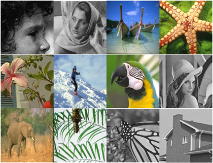
In this section, the experimental results obtained from the proposed model (16) are presented and compared with the SR + TGV method [23] and the TGV method [19]. A total of 12 natural images, as depicted in Figure 2 , were tested, assuming that the pixel value range in clean images is $[0,255]$. The dimensions of three images (FishingBoat, Skiing, and Elephant) are $481 \times 321$, while the remaining nine images have dimensions of $256 \times 256$. For this experiment, the degradation $y=H x+\eta=H x+\gamma \frac{\eta_1}{\eta_2}$ is employed to generate images with Cauchy noise, in which represents a Cauchy distribution, denotes the noise level, and $\eta_1, \eta_2$ are independent random variables following Gaussian distribution with a mean of 0 and a variance of 1 , respectively. In the denoising case, is an identity operation, and is only contaminated with Cauchy noise. Thus, the degradation $y=x+\eta=x+\gamma \frac{\eta_1}{\eta_2}$ is utilized to generate noisy images $\mathrm{y}$.
|
Algorithm 1: Algorithm for solving model (16) proposed in this paper |
|
Step 1. Input: Observed image y, degradation matrix H, parameters λ0, λ, μ, total number of image block groups n, image block size, number of image blocks per group, number of dictionary columns, number of inner-loop iterations, convergence threshold tol, growth rate $r_\beta, r_{\Upsilon_1}, r_{\Upsilon_2}, r_{\xi}$ Step 2: Initialization x=max(min(y,255),0) D=DCT i=1 Step 3: while i<=n do Step 4: t=0 Step 5: Initialization $\beta, \Upsilon_1, \Upsilon_2, \xi$ and $x_{G_i}^t=\mathrm{R}_{G_i}(x)$, $\mathrm{y}_{G_i}=\mathrm{R}_{G_i}(y)$, $\mathrm{D}_{G_i}=\mathrm{R}_{G_i}(D), p=\mathrm{x}_{G_i}^t, \mathrm{w}_j^t=0(j \in\{1,2,3,4\}), q_j^t=\left(\nabla_j x_{G_i}^t-w_j^t\right)(j \in\{1,2,3,4\})$, $\varepsilon\left(w^t\right)_j=\nabla_j w_j^t+\sum_{i=1 \text { and } i \neq j}^4 \frac{\nabla_i}{2} w_j^t(j \in\{1,2,3,4\})$, $r_j^t=\varepsilon\left(w^t\right)_j(j \in\{1,2, \cdots, 16\}), z=H x_{G_i}^t$ step 6: for t<=TI and $\frac{\left\|\hat{x}_{G_i}^t-\hat{x}_{G_i}^{t-1}\right\|_2}{\left\|\hat{x}_{G_i}^t\right\|_2}>t o l$ Step 7: t=t+1 Step 8: Update $a_{G_i}^t$ with OMP solving the solution of (26) Step 9: $p^t=(2 I+\beta I)^{-1}\left(2 D_{G_i} a_{G_i}^t+\beta x_{G_i}^{t-1}\right)$ Step 10: Update $z^t$ by using Newton method to solve the solution of Eq. (28) Step 11: $q_j^t=\left(\Upsilon_1 I+\lambda_1 \Lambda\left(q_j^{t-1}\right)^T \Lambda\left(q_j^{t-1}\right)\right)^{-1} \Upsilon_1\left(\nabla_j x_{G_i}^{t-1}-w_j^{t-1}\right)$ Step 12: $r_j^t=\left(\Upsilon_2 I+\lambda_0 \Lambda\left(r_j^{t-1}\right)^T \Lambda\left(r_j^{t-1}\right)\right)^{-1} \Upsilon_2 \varepsilon\left(w^{t-1}\right)_j$ Step 13: Obtain $x_{G_i}^t$ by using FFT to solve the solution of (33) Step 14: Obtain $w_j^t(j \in\{1,2,3,4\})$ by using FFT to solve the solutions of Eqns. (34)-(37) Step 15: Update dictionary $D_{G_i}$ with KSVD Step 16: $\beta=\beta \cdot r_\beta, \Upsilon_1=\Upsilon_1 \cdot r_{\Upsilon_1}, \Upsilon_2=\Upsilon_2 \cdot r_{\Upsilon_2}, \xi=\xi \cdot r_{\xi}$ Step 17: end for Step 18: i=i+1 Step 19: end while Step 20: Output: restored image $\hat{x}=\left(\sum_{i=1}^n R_{G_i}^T R_{G_i}\right)^{-1} \sum_{i=1}^n R_{G_i}^T\left(x_{G_i}\right)$ |
The PSNR and SSIM values are computed to evaluate the quality of the recovered images, with the calculation formula provided in (38).
$\operatorname{PSNR}(\mathrm{x}, \hat{\mathrm{x}})=$$10{{\log }_{10}}\left( \frac{\max _{x,\hat{x}}^{2}}{\left\| x-\hat{x} \right\|_{2}^{2}} \right),\text{ }SSIM=\frac{2Mea{{n}_{X}}Mea{{n}_{{\hat{x}}}}\left( 2\sigma +{{C}_{2}} \right)}{\left( Mean_{x}^{2}+Mean_{{\hat{x}}}^{2}+{{C}_{1}} \right)\left( \sigma _{x}^{2}+\sigma _{{\hat{x}}}^{2}+{{C}_{2}} \right)},$ (38)
where, $\mathrm{x}, \hat{\mathrm{x}}$ represent the original clean image and its corresponding recovered image, respectively. $\max _{x, \hat{x}}$ denotes the largest pixel value in image $\mathrm{x}, \hat{\mathrm{x}}$, Mean $n_X$ and Mean $_{\hat{x}}$ represent the mean value of $\mathrm{x}, \hat{\mathrm{x}}$, and $\sigma_x^2$, $\sigma_{\widehat{x}}^2$ represent the variance of $\mathrm{x}, \hat{\mathrm{x}}$, respectively, $\sigma$ is the covariance of $\mathrm{x}, \hat{\mathrm{x}}$, and $C_1, C_2$ are constants greater than 0 . A higher PSNR value and an SSIM value closer to 1 indicate that the restored image is more similar to its corresponding original clean image.
4.1 Parameter settings for the experiment
For this experiment, the image block size is set to $4 \times 4$, while the group size is configured as $16 \times 60$. Each group contains 60 image blocks, with 2 overlapping pixels between adjacent image blocks. A search window of $40 \times 40$ is employed, and the size of each dictionary is established as $16 \times 256$. Initial values for penalty parameters are given as $\left(\beta, \Upsilon_1, \Upsilon_2, \xi\right)=(1,0.1,0.1,10)$, with growth rates assigned as $\left(r_\beta, r_{\Upsilon_1}, r_{\Upsilon_2}, r_{\xi}\right)=(2 \%, 3 \%$ , $3 \%, 2 \%$ ). In the denoising scenario, the regularization parameters are set to 6 and 30 , while for deblurring they are 0.2 and 1. Parameters $\lambda$ and $\mu_{G_i}$ are adjusted according to the noise level. For example, when the noise level $\gamma=0.02, \lambda \in\{3,3.5,4,4.5,5,5.5,6\}$ and $\mu_{G_i}=6.25$. If the noise level $\gamma=0.04, \lambda \in\{4,4.5,5,5.5,6,6.5,7\}$ and $\mu_{G_i}=3.125$. When the noise level $\gamma=0.08, \lambda \in\{5,5.5,6,6.5,7,7.5,8\}$ and $\mu_{G_i}=1.5625$. The initial value of $x$ is set as $\max (\min (y, 255), 0)$, following the approach of $[2]$.
4.2 Image denoising results and analysis
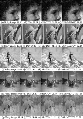
Initially, denoising results obtained by the TGV method, the SR+TGV method, and the proposed GSR+MDTGV method are compared in Figure 3 to Figure 8. The SR+TGV method combines the prior of sparse representation with TGV regularization, while the proposed GSR+MDTGV method incorporates the prior of group sparse representation with MDTGV regularization. Figure 3 displays denoised images produced by the three methods with a Cauchy noise level of γ=0.02.
It is evident from the results that the SR+TGV method improves upon the TGV method by restoring more texture without the staircase effect. The SR+TGV method also includes the prior of sparse representation, which better preserves texture in the uniform region by fully denoising it. This demonstrates the advantage of the sparse prior based on image blocks. In contrast, the denoised results of GSR+MDTGV and SR+TGV appear similar, but the GSR+MDTGV method yields clearer texture details, as demonstrated in the locally zoomed areas of restored images in Figure 4. Additionally, the proposed GSR+MDTGV method introduces two diagonal gradients compared to SR+TGV, recovering more edge features such as the texture area of Lena's brim and the shadow part of FishingBoat's bow, resulting in higher PSNR values. As the noise level increases, these phenomena become more apparent.
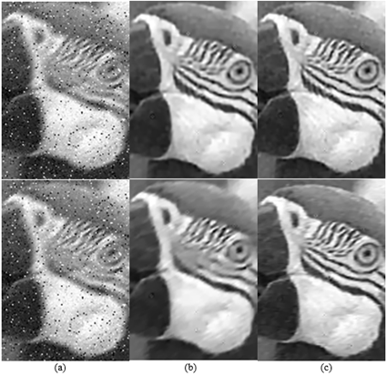
In Figure 5 and Figure 6, denoised results of the TGV, SR+TGV, and GSR+MDTGV methods are compared when the noise level is γ=0.04. The proposed GSR+MDTGV method retains more texture and detail, offering a more natural visual quality. This is attributed to the fact that GSR+MDTGV provides more information on similar image block structures than SR+TGV, as shown in the locally zoomed areas of restored images in Figure 6. For example, the texture area of white hair beneath the parrots, the details of the scarf texture area on Barbara's right shoulder, and the protruding bone texture in the starfish are more distinct, resulting in higher PSNR values.
Lastly, in Figure 7 and Figure 8, denoised images obtained by the TGV, SR+TGV, and GSR+MDTGV methods are compared when the noise level is high (i.e., γ=0.04 or 0.08). It can be observed that the image backgrounds restored by the TGV and SR+TGV methods are rough. However, the proposed method ensures smoothness in the background and further enhances the visual quality of natural images. These experiments confirm the advantages of GSR+MDTGV regularization compared to other prior knowledge. Specifically, although the restored results using GSR+MDTGV and SR+TGV are visually similar, GSR+MDTGV better preserves texture and detail, providing more visually natural images and achieving higher PSNR values.
Figure 2. Original clean images. Top to bottom (left to right): Girl, Barbara, FishingBoat(481×321), Starfish, Flower, Skiing(481×321), Parrot, Lena, Elephant(481×321), Leave, Butterfly, House
Figure 3. Results of recovered images obtained by different methods for eliminating Cauchy noise. The number under each image is the PSNR (dB) value. First column: noisy images (γ = 0.02); second column: recovered images using the TGV method; third column: recovered images using the SR+TGV method; fourth column: recovered images using our GSR+MDTGV method
Table 1. Denoised results when noise level γ = 0.02
|
Model |
(a) TGV model |
(b) SR+TGV model |
(c) Proposed model |
|||
|
Image |
PSNR |
SSIM |
PSNR |
SSIM |
PSNR |
SSIM |
|
Girl |
28.29 |
0.9205 |
29.78 |
0.9405 |
31.65 |
0.9592 |
|
Barbara |
25.26 |
0.7702 |
28.38 |
0.8453 |
30.24 |
0.8912 |
|
FishingBoat |
28.67 |
0.7613 |
29.74 |
0.7920 |
31.98 |
0.8544 |
|
Starfish |
30.02 |
0.8458 |
31.08 |
0.8912 |
32.97 |
0.9132 |
|
Flower |
30.21 |
0.8588 |
32.18 |
0.9038 |
32.65 |
0.8987 |
|
Skiing |
29.82 |
0.9052 |
31.25 |
0.9232 |
33.60 |
0.9459 |
|
Parrot |
30.43 |
0.8502 |
32.01 |
0.8699 |
33.09 |
0.9012 |
|
Lena |
30.63 |
0.8823 |
31.16 |
0.8736 |
32.14 |
0.9088 |
|
Elephant |
29.69 |
0.7684 |
31.11 |
0.8237 |
33.29 |
0.8846 |
|
Leave |
27.98 |
0.9102 |
30.45 |
0.9417 |
31.78 |
0.9599 |
|
Butterfly |
28.27 |
0.8641 |
30.10 |
0.8862 |
32.42 |
0.9285 |
|
House |
30.48 |
0.9045 |
32.86 |
0.9204 |
32.29 |
0.9016 |
Figure 4. Local zoomed areas of recovered images in Figure 3. (a) original images, (b) recovered images using the TGV method, (c) recovered images using the SR+TGV method, and (d) recovered images using our GSR+MDTGV method
Table 1 to Table 3 present the PSNR and SSIM values of the restored results obtained using the different methods. In most cases, the proposed model yields the highest values for both PSNR and SSIM. In general, the proposed model achieves superior denoising results based on these image quality measurements, which is closely related to the exceptional performance of the regularization model founded on group sparse representation prior and multi-directional total generalized variation.
Table 2. Denoised results when noisy level γ =0.04
|
Model |
(a) TGV model |
(b) SR+TGV model |
(c) Proposed model |
|||
|
Image |
PSNR |
SSIM |
PSNR |
SSIM |
PSNR |
SSIM |
|
Girl |
27.41 |
0.7912 |
28.69 |
0.8978 |
30.43 |
0.9309 |
|
Barbara |
23.47 |
0.7318 |
27.60 |
0.8242 |
28.84 |
0.8588 |
|
FishingBoat |
27.42 |
0.7414 |
28.70 |
0.7709 |
29.97 |
0.8099 |
|
Starfish |
28.04 |
0.8383 |
29.25 |
0.8663 |
31.48 |
0.9089 |
|
Flower |
28.11 |
0.8088 |
29.78 |
0.8538 |
30.65 |
0.8487 |
|
Skiing |
28.69 |
0.8765 |
29.45 |
0.8956 |
30.23 |
0.9102 |
|
Parrot |
29.32 |
0.8389 |
30.11 |
0.8456 |
31.14 |
0.8584 |
|
Lena |
28.11 |
0.7988 |
28.90 |
0.8155 |
28.48 |
0.8065 |
|
Elephant |
29.57 |
0.7753 |
30.12 |
0.7980 |
30.91 |
0.8266 |
|
Leave |
26.72 |
0.8946 |
28.14 |
0.9158 |
30.60 |
0.9469 |
|
Butterfly |
27.19 |
0.8542 |
29.38 |
0.8864 |
31.58 |
0.9179 |
|
House |
28.77 |
0.7745 |
29.86 |
0.7834 |
30.99 |
0.8016 |
Figure 5. Results of recovered images obtained by different methods for eliminating Cauchy noise. The number under each image is the PSNR (dB) value. First column: noisy images (γ = 0.04); second column: recovered images using the TGV method; third column: recovered images using the SR+TGV method; fourth column: recovered images using our GSR+MDTGV method
Table 3. Denoised results when noisy level γ = 0.08
|
Model |
(a) TGV model |
(b) SR+TGV model |
(c) Proposed model |
|||
|
Image |
PSNR |
SSIM |
PSNR |
SSIM |
PSNR |
SSIM |
|
Girl |
25.59 |
0.5955 |
26.22 |
0.6611 |
28.96 |
0.7502 |
|
Barbara |
22.63 |
0.6932 |
26.57 |
0.7827 |
27.41 |
0.8113 |
|
FishingBoat |
26.62 |
0.7217 |
26.77 |
0.7258 |
27.10 |
0.7344 |
|
Starfish |
26.87 |
0.7312 |
27.84 |
0.7810 |
30.03 |
0.8492 |
|
Flower |
25.99 |
0.7569 |
27.56 |
0.7985 |
28.34 |
0.8126 |
|
Skiing |
26.36 |
0.8312 |
27.96 |
0.8589 |
29.16 |
0.8898 |
|
Parrot |
27.42 |
0.8087 |
29.11 |
0.8299 |
30.22 |
0.8490 |
|
Lena |
26.16 |
0.7550 |
26.56 |
0.7650 |
27.51 |
0.7862 |
|
Elephant |
27.78 |
0.6868 |
28.23 |
0.7115 |
28.49 |
0.7253 |
|
Leave |
24.84 |
0.8519 |
26.02 |
0.8865 |
28.58 |
0.9201 |
|
Butterfly |
25.82 |
0.8099 |
26.85 |
0.8278 |
27.07 |
0.8354 |
|
House |
27.09 |
0.5628 |
28.00 |
0.7565 |
28.90 |
0.6595 |
Figure 6. Local zoomed areas of recovered images in Figure 5. (a) original images, (b) recovered images using the TGV method, (c) recovered images using the SR+TGV method, and (d) recovered images using our GSR+MDTGV method
Figure 7. Comparison of denoising results when γ = 0.04 (Rows 1 and 3), γ = 0.08 (Rows 2 and 4) with different regularization terms (TGV, SR+TGV, GSR+MDTGV) and the same data fidelity term in (16). PSNR: (top) (a) 28.77, (b) 29.86, (c) 30.99; (row 2) (a) 27.09, (b) 28.03, (c) 28.90; (row 3) (a) 28.11, (b) 29.78, (c) 30.65; (bottom) (a) 25.99, (b) 27.56, (c) 28.34
Figure 8. Local zoomed areas of the recovered house images when γ = 0.08 in Figure 7
Table 4. Comparisons of the performance of SR+TGV and our GSR+MDTGV method on PSNR, SSIM, and Time (in minutes) when noisy level γ =0.08
|
Image |
SR+TGV |
Ours |
||||
|
PSNR |
SSIM |
Time |
PSNR |
SSIM |
Time |
|
|
Parrot |
29.11 |
0.8299 |
0.78 |
30.22 |
0.8490 |
0.59 |
|
Flower |
27.56 |
0.7985 |
0.80 |
28.34 |
0.8126 |
0.61 |
|
Lena |
26.56 |
0.7650 |
0.99 |
27.51 |
0.7862 |
0.79 |
Finally, a comparison is made between the PSNR, SSIM, and time (in minutes) values of the SR + TGV and GSR + MDTGV methods in Table 4. Three images corrupted by the Cauchy noise level γ = 0.08 are selected for testing. The results show that the GSR + MDTGV method achieves higher values of PSNR and SSIM and runs faster, indicating that the computing time for group sparse representation is less than that of global sparse representation.
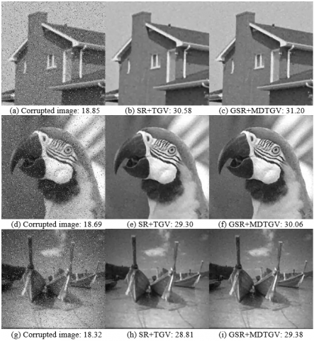
Figure 9. Restored images from deblurring-denoising images contaminated with one Gaussian blur and Cauchy noise using the SR+TGV and our GSR+MDTGV methods
Figure 10. Recovered images from deblurring-denoising images contaminated with one motion blur and Cauchy noise using the SR+TGV and our GSR+MDTGV methods
Table 5. The values of PSNR (dB) and SSIM of deblurring-denoising results with noise level γ = 0.02 and different blurring kernels using the SR+TGV and GSR+MDTGV methods
|
Corrupted |
Gaussian blur and Cauchy noise |
Motion blur and Cauchy noise |
||||||
|
Method |
SR+TGV |
Ours |
SR+TGV |
Ours |
||||
|
Image |
PSNR |
SSIM |
PSNR |
SSIM |
PSNR |
SSIM |
PSNR |
SSIM |
|
Girl |
28.71 |
0.8968 |
29.79 |
0.9389 |
25.93 |
0.6320 |
26.34 |
0.6912 |
|
Barbara |
27.80 |
0.8339 |
28.87 |
0.8319 |
26.02 |
0.8149 |
27.79 |
0.8330 |
|
FishingBoat |
28.81 |
0.7958 |
29.38 |
0.8055 |
27.98 |
0.7743 |
29.01 |
0.7950 |
|
Starfish |
29.12 |
0.8834 |
31.03 |
0.8905 |
28.85 |
0.8598 |
29.05 |
0.8581 |
|
Flower |
30.25 |
0.8598 |
30.02 |
0.8499 |
27.69 |
0.8289 |
27.98 |
0.8395 |
|
Skiing |
29.75 |
0.9045 |
31.02 |
0.9098 |
27.32 |
0.8778 |
28.12 |
0.8891 |
|
Parrot |
29.30 |
0.8502 |
30.06 |
0.8421 |
26.62 |
0.8303 |
29.36 |
0.8269 |
|
Lena |
29.09 |
0.8197 |
30.01 |
0.8213 |
27.78 |
0.8059 |
27.32 |
0.8012 |
|
Elephant |
29.43 |
0.8082 |
31.09 |
0.8109 |
28.09 |
0.7769 |
28.72 |
0.7906 |
|
Leave |
28.47 |
0.9195 |
29.99 |
0.9275 |
27.38 |
0.9079 |
28.69 |
0.9208 |
|
Butterfly |
28.35 |
0.9208 |
29.25 |
0.9302 |
26.59 |
0.8997 |
27.80 |
0.9042 |
|
House |
30.58 |
0.8241 |
31.20 |
0.8216 |
29.83 |
0.8143 |
30.86 |
0.8247 |
4.3 Image deblurring-denoising results and analysis
In this section, the restoration of images contaminated with Cauchy noise and blur is considered. Two blur kernels are examined: a Gaussian blur kernel with a size of 8x8 and a standard deviation of 1, and a motion blur kernel with len = 9 and theta = 50. Subsequently, Cauchy noise with a noise level γ = 0.02 is added to the blurred images.
Three images are selected for testing, and the restored results of deblurring-denoising are displayed in Figure 9 and Figure 10. The values of PSNR and SSIM obtained using different methods in the two blur kernels and various noise levels are listed in Table 5 and Table 6. It is evident from Tables 5 and 6 that the proposed GSR + MDTGV method achieves relatively high values of PSNR and SSIM. The images in Figure 9 and Figure 10 reveal that the images restored using the SR + TGV and GSR + MDTGV methods are visually similar, but the GSR + MDTGV method consistently obtains higher PSNR values and clearer texture features. This is particularly apparent in the local zoomed area of the restored parrot image from Figure 11, such as the texture area of white hair under the parrots. As a result, the GSR + MDTGV method not only retains good texture features but also effectively removes blur and Cauchy noise. This is closely related to the outstanding performance of the regularization model based on group sparse representation prior and multi-directional total generalized variation.
Table 6. The values of PSNR (dB) and SSIM of deblurring-denoising results with noisy level γ = 0.04 and different blurring kernels using the SR+TGV and our GSR+MDTGV methods
|
Corrupted |
Gaussian blur and Cauchy noise |
Motion blur and Cauchy noise |
||||||
|
Method |
SR+TGV |
Ours |
SR+TGV |
Ours |
||||
|
Image |
PSNR |
SSIM |
PSNR |
SSIM |
PSNR |
SSIM |
PSNR |
SSIM |
|
Girl |
27.52 |
0.8038 |
28.89 |
0.8689 |
24.23 |
0.492 |
24.84 |
0.5862 |
|
Barbara |
27.20 |
0.8130 |
27.93 |
0.8053 |
25.12 |
0.7836 |
26.38 |
0.7930 |
|
FishingBoat |
27.82 |
0.7737 |
27.75 |
0.7655 |
26.50 |
0.7412 |
26.57 |
0.7350 |
|
Starfish |
28.04 |
0.8467 |
30.05 |
0.8692 |
27.23 |
0.8047 |
27.58 |
0.8261 |
|
Flower |
28.71 |
0.8247 |
28.58 |
0.8212 |
25.38 |
0.7763 |
25.83 |
0.7965 |
|
Skiing |
28.65 |
0.8831 |
29.54 |
0.8911 |
25.68 |
0.8456 |
25.90 |
0.8610 |
|
Parrot |
28.33 |
0.8369 |
29.10 |
0.8247 |
25.17 |
0.8103 |
27.93 |
0.8008 |
|
Lena |
27.56 |
0.7835 |
28.47 |
0.7804 |
25.48 |
0.7399 |
25.01 |
0.7516 |
|
Elephant |
28.47 |
0.7708 |
29.49 |
0.7578 |
26.32 |
0.7110 |
26.65 |
0.7208 |
|
Leave |
26.99 |
0.9011 |
28.92 |
0.9142 |
25.17 |
0.8803 |
27.09 |
0.9009 |
|
Butterfly |
27.27 |
0.8992 |
27.47 |
0.9013 |
24.97 |
0.8705 |
25.13 |
0.8576 |
|
House |
28.96 |
0.7695 |
30.07 |
0.7409 |
27.40 |
0.7036 |
29.17 |
0.7323 |
Figure 11. Local zoomed areas of the recovered parrot images in Figure 9 and Figure 10. (a) Corrupted image, (b) recovered images using the SR+TGV method, (c) recovered images using the GSR+MDTGV method
In this study, a model fusing the prior knowledge of GSR and MDTGV is proposed to restore images contaminated with Cauchy noise and/or blur. The model is solved using a penalty method, variable splitting strategy, and alternating minimization scheme. The prior knowledge of GSR leverages the nonlocal self-similarity of images by considering the non-zero coefficients appearing in the form of clustering in sparse representation signals. This approach takes into account the sparsity of the group structure, preserves more geometric structures, and requires less computation time than global sparse representation. MDTGV regularization can describe the edge information in 8 directions of the image and reconstruct clearer detailed features, resulting in ideal visual results and better visual quality than TGV. Experimental results demonstrate that the proposed method outperforms comparison methods in terms of PSNR and SSIM values in most cases. It is important to note that in these methods, the Cauchy noise level and blur kernel are known; however, in real corrupted images, the Cauchy noise level and blur kernel may be unknown.
To address this limitation, future work will focus on improving the GSR + MDTGV method to adapt to nonparametric blind super-resolution, where the noise level and blur kernel are unknown. Initially, methods will be employed to estimate the noise level and blur kernel size. Subsequently, given the estimated noise level and blur kernel, the SR method based on GSR+MDTGV will be used to super-resolve the final high-resolution image. This extension of the proposed method has the potential to enhance its applicability in various real-world scenarios where the noise level and blur kernel are not readily available.
This work is supported by the Natural Science Foundation of Zhejiang Province (Grants No.: LGG22F020040, LZ21F020001, and LD21F020001); National Social Science Foundation of China (Grant No.: 19BTJ031); The project of Wenzhou Key Laboratory Foundation (Grant No.: 2021HZSY0071); The Key scientific and technological innovation projects of Wenzhou Science and Technology Plan (Grant No.: ZY2019020).
[1] Sciacchitano, F., Dong, Y., Zeng, T. (2015). Variational approach for restoring blurred images with Cauchy noise. SIAM Journal on Imaging Sciences, 8(3): 1894-1922. https://doi.org/10.1137/140997816
[2] Mei, J.J., Dong, Y., Huang, T.Z., Yin, W. (2018). Cauchy noise removal by nonconvex ADMM with convergence guarantees. Journal of Scientific Computing, 74: 743-766. https://doi.org/10.1007/s10915-017-0460-5
[3] Zhao, P., Zhao, X., Zhao, C. (2020). Image denoising based on bivariate distribution. Symmetry, 12(11): 1909. https://doi.org/10.3390/sym12111909
[4] Hill, P.R., Achim, A.M., Bull, D.R., Al-Mualla, M.E. (2014). Dual-tree complex wavelet coefficient magnitude modelling using the bivariate Cauchy–Rayleigh distribution for image denoising. Signal Processing, 105: 464-472. https://doi.org/10.1016/j.sigpro.2014.03.028
[5] Wu, T., Li, W., Jia, S., Dong, Y., Zeng, T. (2020). Deep multi-level wavelet-cnn denoiser prior for restoring blurred image with cauchy noise. IEEE Signal Processing Letters, 27: 1635-1639. https://doi.org/10.1109/LSP.2020.3023299
[6] Rudin, L.I., Osher, S., Fatemi, E. (1992). Nonlinear total variation based noise removal algorithms. Physica D: Nonlinear Phenomena, 60(1-4): 259-268. https://doi.org/10.1016/0167-2789(92)90242-F
[7] Wang, Y., Yin, W., Zeng, J. (2019). Global convergence of ADMM in nonconvex nonsmooth optimization. Journal of Scientific Computing, 78: 29-63. https://doi.org/10.1007/s10915-018-0757-z
[8] Yang, J.H., Zhao, X.L., Mei, J.J., Wang, S., Ma, T.H., Huang, T.Z. (2019). Total variation and high-order total variation adaptive model for restoring blurred images with Cauchy noise. Computers & Mathematics with Applications, 77(5): 1255-1272. https://doi.org/10.1016/j.camwa.2018.11.003
[9] Parisotto, S., Lellmann, J., Masnou, S., Schonlieb, C.B. (2020). Higher-order total directional variation: Imaging applications. SIAM Journal on Imaging Sciences, 13(4): 2063-2104. https://doi.org/10.1137/19M1239209
[10] Shi, K., Dong, G., Guo, Z. (2020). Cauchy noise removal by nonlinear diffusion equations. Computers & Mathematics with Applications, 80(9): 2090-2103. https://doi.org/10.1016/j.camwa.2020.08.027
[11] Liu, Q., Gao, S. (2020). Directional fractional-order total variation hybrid regularization for image deblurring. Journal of Electronic Imaging, 29(3): 033001-033001. https://doi.org/10.1117/1.JEI.29.3.033001
[12] Bredies, K., Kunisch, K., Pock, T. (2010). Total generalized variation. SIAM Journal on Imaging Sciences, 3(3): 492-526. https://doi.org/10.1137/090769521
[13] Lv, Y. (2020). Total generalized variation denoising of speckled images using a primal-dual algorithm. Journal of Applied Mathematics and Computing, 62(1-2): 489-509. https://doi.org/10.1007/s12190-019-01293-8
[14] Shi, Y., Zhang, X., Rao, Z., Wang, M., Soleimani, M. (2019). Reduction of staircase effect with total generalized variation regularization for electrical impedance tomography. IEEE Sensors Journal, 19(21): 9850-9858. https://doi.org/10.1109/JSEN.2019.2926232
[15] Zhong, Q., Wu, C., Shu, Q., Liu, R.W. (2018). Spatially adaptive total generalized variation-regularized image deblurring with impulse noise. Journal of Electronic Imaging, 27(5): 053006-053006. https://doi.org/10.1117/1.JEI.27.5.053006
[16] Kongskov, R.D., Dong, Y., Knudsen, K. (2019). Directional total generalized variation regularization. BIT Numerical Mathematics, 59(4): 903-928. https://doi.org/10.1007/s10543-019-00755-6
[17] Li, S., Zhang, B., Yang, X., Zhu, W. (2020). Edge-guided second-order total generalized variation for Gaussian noise removal from depth map. Scientific Reports, 10(1): 16329. https://doi.org/10.1038/s41598-020-73342-3
[18] Guo, K., Labate, D. (2007). Optimally sparse multidimensional representation using shearlets. SIAM journal on mathematical analysis, 39(1): 298-318. https://doi.org/10.1137/060649781
[19] Lv, Y. (2020). Shearlet-TGV based model for restoring noisy images corrupted by Cauchy noise. Nonlinear Differential Equations and Applications NoDEA, 27(2): 21. https://doi.org/10.1007/s00030-020-0623-1
[20] Liu, X. (2019). Total generalized variation and wavelet frame-based adaptive image restoration algorithm. The Visual Computer, 35(12): 1883-1894. https://doi.org/10.1007/s00371-018-1581-z
[21] Zhu, J., Li, K., Hao, B. (2019). Image restoration by second-order total generalized variation and wavelet frame regularization. Complexity, 2019: 1-16. https://doi.org/10.1155/2019/3650128
[22] Zhang, H.T., Yu, J., Wang, Z.F. (2018). Probability contour guided depth map inpainting and superresolution using non-local total generalized variation. Multimedia Tools and Applications, 77: 9003-9020. https://doi.org/10.1007/s11042-017-4791-x
[23] Jung, M., Kang, M. (2021). Image restoration under Cauchy noise with sparse representation prior and total generalized variation. Journal of Computational Mathematics, 39(1): 81. https://doi.org/10.4208/jcm.1907-m2018-0234
[24] Zhang, H., Tang, L., Fang, Z., Xiang, C., Li, C. (2018). Nonconvex and nonsmooth total generalized variation model for image restoration. Signal Processing, 143: 69-85. https://doi.org/10.1016/j.sigpro.2017.08.021
[25] Chen, Y., Peng, Z., Li, M., Yu, F., Lin, F. (2019). Seismic signal denoising using total generalized variation with overlapping group sparsity in the accelerated ADMM framework. Journal of Geophysics and Engineering, 16(1): 30-51. https://doi.org/10.1093/jge/gxy003
[26] Ding, M., Huang, T.Z., Ma, T.H., Zhao, X.L., Yang, J.H. (2020). Cauchy noise removal using group-based low-rank prior. Applied Mathematics and Computation, 372: 124971. https://doi.org/10.1016/j.amc.2019.124971
[27] Laus, F., Pierre, F., Steidl, G. (2018). Nonlocal myriad filters for Cauchy noise removal. Journal of Mathematical Imaging and Vision, 60: 1324-1354. https://doi.org/10.1007/s10851-018-0816-y
[28] Kim, G., Cho, J., Kang, M. (2020). Cauchy noise removal by weighted nuclear norm minimization. Journal of Scientific Computing, 83: 1-21. https://doi.org/10.1007/s10915-020-01203-2
[29] Zhang, J., Zhao, D., Gao, W. (2014). Group-based sparse representation for image restoration. IEEE transactions on image processing, 23(8): 3336-3351. https://doi.org/10.1109/TIP.2014.2323127
[30] Zhang, K.S., Zhong, L., Zhang, X.Y. (2018). Image restoration via group l 2, 1 norm-based structural sparse representation. International Journal of Pattern Recognition and Artificial Intelligence, 32(4): 1854008. https://doi.org/10.1142/S0218001418540083
[31] Ding, M., Huang, T.Z., Wang, S., Mei, J.J., Zhao, X.L. (2019). Total variation with overlapping group sparsity for deblurring images under Cauchy noise. Applied Mathematics and Computation, 341: 128-147. https://doi.org/10.1016/j.amc.2018.08.014
[32] Lee, S., Kang, M. (2020). Group sparse representation for restoring blurred images with Cauchy noise. Journal of Scientific Computing, 83: 1-27. https://doi.org/10.1007/s10915-020-01227-8
[33] Lin, J., Deng, D., Yan, J., Lin, X. (2017). Self-adaptive group based sparse representation for image inpainting. Journal of Computer Applications, 37(4): 1169-1173.
[34] Yang, M., Ling, G., Zhao, F.C. (2018). Self-adaptive group sparse representation method for image inpainting. Computer Science, 45(8): 272-276.
[35] Mo, J., Zhou, Y. (2019). The research of image inpainting algorithm using self-adaptive group structure and sparse representation. Cluster Computing, 22: 7593-7601. https://doi.org/10.1007/s10586-018-2323-8
[36] Kumar, A., Ahmad, M.O., Swamy, M.N.S. (2019). Image denoising via overlapping group sparsity using orthogonal moments as similarity measure. ISA Transactions, 85: 293-304. https://doi.org/10.1016/j.isatra.2018.10.030
[37] Xu, S.H., Gao, F. (2017). Single-image super resolution based on group sparse representation via gaussian. International Journal of Circuits, Systems and Signal Processing, 11: 118-128.
[38] Csiszár, I. (1984). Information geometry and alternating minimization procedures. Statistics and Decisions, Dedewicz, 1: 205-237.
[39] Liu, J., Huang, T.Z., Selesnick, I.W., Lv, X.G., Chen, P.Y. (2015). Image restoration using total variation with overlapping group sparsity. Information Sciences, 295: 232-246. https://doi.org/10.1016/j.ins.2014.10.041
[40] Park, S.W., Park, J., Jung, B.C. (2013). On the sparse signal recovery with parallel orthogonal matching pursuit. IEICE Transactions on Fundamentals of Electronics, Communications and Computer Sciences, 96(12): 2728-2730. https://doi.org/10.1587/transfun.E96.A.2728
[41] Aharon, M., Elad, M., Bruckstein, A. (2006). K-SVD: An algorithm for designing overcomplete dictionaries for sparse representation. IEEE Transactions on Signal Processing, 54(11): 4311-4322. https://doi.org/10.1109/TSP.2006.881199
[42] Chen, P.Y., Selesnick, I.W. (2014). Translation-invariant shrinkage/thresholding of group sparse signals. Signal Processing, 94: 476-489. https://doi.org/10.1016/j.sigpro.2013.06.011
[43] Hunter, D.R., Lange, K. (2004). A tutorial on MM algorithms. The American Statistician, 58(1): 30-37. https://doi.org/10.1198/0003130042836
[44] Figueiredo, M.A., Bioucas-Dias, J.M., Nowak, R.D. (2007). Majorization–minimization algorithms for wavelet-based image restoration. IEEE Transactions on Image Processing, 16(12): 2980-2991. https://doi.org/10.1109/TIP.2007.909318
[45] Nocedal, J., Wright, S.J., Mikosch, T.V., Resnick, S.I., Robinson, S.M. (1999). Numerical optimization. New York, NY: Springer New York.
[46] Wang, Y., Yang, J., Yin, W., Zhang, Y. (2008). A new alternating minimization algorithm for total variation image reconstruction. SIAM Journal on Imaging Sciences, 1(3): 248-272. https://doi.org/10.1137/080724265