Abdulwaheed Adebola Yusuf*![]() | Betul Ay
| Betul Ay![]() | Guven Fidan
| Guven Fidan![]() | Galip Aydin
| Galip Aydin![]()
© 2023 IIETA. This article is published by IIETA and is licensed under the CC BY 4.0 license (http://creativecommons.org/licenses/by/4.0/).
OPEN ACCESS
Zero hunger, the goal 2 of Sustainable Development Goals (SDGs), can only be achieved when food is available, affordable and accessible to the people. Food insecurity, a phenomenon where either or all of these ingredients for zero hunger are absent, remains a critical global issue that warrants coordinated strategies at regional scale; most especially for crop farming which serves as the major source of food for most humans. Therefore, efficient Land Use and Land Cover (LULC) classification is a pivotal tool in the development of apposite strategies for combating food insecurity. Open satellite missions like Sentinel 2 offer a cost effective way for acquiring regional imagery dataset for LULC classification; however, the relevance of such dataset is dependent on the quality of ground truth data from which the imagery dataset is created. Qualitative ground truth data are usually obtained through ground surveys which come at extra costs, warranting the need for elaborate community ground truth geo-database constructed from joint ground surveys. Such database is absent in the tropical belt that is mostly made up of developing countries where higher impacts of food insecurity are experienced. This remained the case, until recently when JECAM (Joint Experiment for Crop Assessment and Monitoring) database was developed for six countries in the tropical belt. JECAM database is an elaborate geo-database that consists of 27,074 agricultural LULC polygons (20,257 crops and 6,817 non crops). In this study, we built three deep learning models for agricultural LULC classification using the entire 13 bands of the satellite imagery dataset. Class-based performance evaluation metrics were used to evaluate the performances of the deep learning models on test set. LSTM (Long Short-Term Memory) model exhibited the highest capability for LULC class discrimination, followed by 2D-CNN (2 Dimension Convolution Neural Network) Autoencoder model, then the 2D-CNN model. In the future, we intend to exploit spectral indices and transfer learning paradigm to address class imbalance problem, which is inherent in the imagery dataset, for improved LULC class discrimination.
land cover, deep learning, convolution neural network, autoencoder, long short-term memory
Food insecurity is a global crisis that impacts over 800 million people to be either hungry or malnourished [1], warranting efficient and pragmatic agricultural strategies at regional scale. Accurate generation of Land Use and Land Cover (LULC) maps is fundamental to these strategies as they provide holistic views to evaluate land changes resulting from both natural and cultural phenomena. LULC classification for automating LULC map generation at regional scale can be achieved using imagery from satellite systems due to their wider imaging coverage and continuous data acquisition for prospective analysis. Deep learning techniques, a subset of machine learning methods developed to effectively overcome the problem of curse of dimensionality [2], have been employed to generate accurate LULC maps from satellite imagery in a number of studies via classification tasks [3-8]; however, it should be noted that the relevance of these satellite imagery are dependent on their conformity to ground truth for an area of interest. Thus, there is need to conduct surveys for obtaining ground truth, which come at prohibitive costs, especially when the area of interest is large. This has inhibited the adoption of satellite imagery for complex agriculture systems in developing countries [9] where impacts of food insecurity are greatly felt.
A cost effective approach for obtaining ground truth is through provision of open database that contains coordinates of area of interest with defined feature(s), gathered via joint physical surveys, which can be used to mask satellite imagery for LULC classification. Adopting this approach, a number of ground truth datasets have been released. However, these datasets are not suitable for developing countries due to exclusive scope of interest, broad taxonomy that reduces a number of agriculture land covers to single class and localization difficulties for crop practices [9]. For instance, a review of ground truth database available for global south has been presented by authors [10], where Land Cover-Climate Change Initiative (LC-CCI), Global Observation for Forest Cover and Land Dynamics (GOFC-GOLD), Food and Agriculture Organisation-Forest Resources Assessment (FAO-FRA) and Geo-Wiki datasets are discussed to have potential for broader applicability for multiple uses. Nevertheless, the wider applicability scope is threatened by absence of information on how these datasets can be used beyond their original scope. Besides, the GOFC-GOLD dataset generally contains a single nomenclature (“crop land” or “cultivated”) for crop types, except for GlobCover 2005 subset which has a “rainfed cropland”, rendering the dataset less useful for applications involving crop mapping [9].
Moreover, the authors [11, 12] collected crowdsourced ground truth dataset via Wiki tool, where the number of cropland samples are fairly large. Nonetheless, these cropland samples are referenced with only one class in the nomenclature. In addition, dataset generated through crowdsourcing are not suitable for circumstances where precise information must be collected in terms of plot boundaries, spatial resolution, and crop type nomenclatures, as crowdsourcing initiatives are principally based on visual interpretation of images which inhibit the identification and precise localization of cropping practices. JECAM ground truth database presented by authors [9] has the potential to address the draw backs of existing ground truth dataset for some developing countries.
Exploiting advancements in computing resources and data modeling algorithms, this study seeks to apply deep learning methods on Sentinel 2 satellite imagery acquired from JECAM open in situ database for agricultural LULC classification. We employed the entire 13 bands of the sentinel 2 L1C data for the classification tasks. The classified LULC maps generated from resulting deep learning models were evaluated using classification metrics.
The rest of this paper is structured as follows. Section 2 presents methodology where the JECAM database, dataset acquisition, modeling method and experiment are discussed. The result of the experiment is presented and discussed in Section 3. Section 4 concludes the paper with recommendations for further research.
2.1 JECAM database
This database is an aggregation of 24 harmonized datasets collected under the Joint Experiment for Crop Assessment and Monitoring (JECAM) initiative, spread across 9 sites in 6 tropical countries; and it consists of 27,074 polygons (20, 257 crops and 6,817 non crops), gathered between 2013 and 2020. (See Table 1 for polygons distribution per country). It supports layered imagery classification tasks for LULC discrimination and crop mapping, providing up to 11 LULC classes (Cropland, Herbaceous savannah, Built-up surface, Savannah with shrubs, Pasture, Mineral soil, Forest, Wetland, Water body, Savannah with trees, and Bare soil) and broader crop types of up to 47, which were majorly acquired through physical surveys [9].
Table 1. Polygons distribution per country
|
Country |
Number of Polygons |
|
Madagascar |
8351 |
|
Burkina Faso |
7114 |
|
Brazil |
6682 |
|
Senegal |
3600 |
|
South Africa |
1741 |
|
Kenya |
1647 |
|
Cambodia |
529 |
The merit of JECAM dataset does not only lies in its inherent quality possessed by its in situ data collection, but also in its large sample size and broader crop classes which present it as a suitable ground truth data source for acquisition of satellite imagery for agricultural systems in developing countries (of the tropical belts), where large ground truth datasets are rare due to mapping difficulty [13], caused by humble sizes of crop fields [14].
2.2 Imagery dataset acquisition
The satellite imagery dataset for this study was acquired from Antsirabe site in Madagascar. It is the only site of Madagascar captured in the JECAM database. Antsirabe, the capital of Vakinankaratra region, is the third biggest city in Madagascar and has a population of 391,000 as at 2022 [15]. It lies on 19°51'57.1"S latitude and 47°1'59.99"E longitude. The Antsirabe site has the maximum number (8351) of polygons and highest percentage (87%) of in situ data collected in the ground truth database. These motivated its choice as study site for this work.
Sentinel 2 L1C imagery dataset from January to December, 2018, was acquired and preprocessed using Google Earth Engine; an open cloud based Geographical Information System (GIS). In order to minimize storage and computational requirements for the imagery data, we averaged [6] reflectance values of the Sentinel 2 L1C images; and we exported the resulting pixel samples in Comma Separated Value (CSV) format for onward processing. The imagery dataset acquisition for this study is divided into two stages which are listed below:
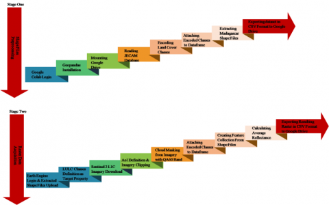
(a) Shape files preprocessing: In order to render shape files stored in the JECAM database suitable for raster data creation, we employed Geopandas library to extract required shape files for our study; and we conducted relevant preprocessing tasks on the shape files using Geopandas and python. These preprocessing tasks were carried out on Google Colab, an open Platform-as-a-Service. Below are steps followed at this stage:
(b) Raster data acquisition: At this stage, raster data for training our models are created using the shape files extracted from the JECAM database for Antsirabe site in Madagascar. Both raster data creation and necessary preprocessing operations to improve ease of computation and LULC classification were carried out on Google Earth Engine following steps listed below:
Figure 1 depicts the diagrammatic view of the imagery data acquisition stages.
Figure 1. Imagery data acquisition
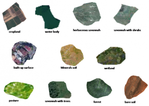
A total of 451, 455 pixels, at a dimension of 13×1, were obtained for this study. The choice of L12C product is due to its support for near real time earth monitoring. Table 2 illustrates pixels sample distribution per LULC class for the satellite dataset, while Figure 2 displays the imagery samples for each LULC class in red, green and blue (RGB) format.
Table 2. Sample distribution per LULC class for satellite imagery dataset
|
LULC Labels |
Number of Pixels |
|
Cropland |
268896 |
|
Water body |
59234 |
|
Herbaceous savannah |
35827 |
|
Savannah with shrubs |
22897 |
|
Built-up surface |
17617 |
|
Mineral soil |
11382 |
|
Wetland |
10980 |
|
Pasture |
10810 |
|
Savannah with trees |
8933 |
|
Forest |
4020 |
|
Bare soil |
859 |
Figure 2. Image samples for LULC classes in RGB format
2.3 Data modeling method
Owing to wider availability of data and improvements in computing resources, Machine Learning, a set of inductive learning techniques that focus on how computers can learn from experience without being explicitly programmed, has recently gained popularity in the data modeling space. However, a major pitfall of machine learning is its inability to effectively model voluminous data with high dimensionality (features), a phenomenon often referred to as curse of dimensionality [16]. This makes machine learning methods less suitable for analysis of satellite images which are characterized with a number of features.
Deep learning, a subset of advanced machine learning methods developed to address the problem of curse of dimensionality, is employed for the modeling of satellite imagery in this work. Deep learning methods are improved Artificial Neural Networks that are stacked with two or more hidden layers for effective feature extraction during inductive learning process [17]. In this study, we adopt three popular deep learning methods, which are Convolution Neural Network (CNN), Long Short-Term Memory (LSTM) and Autoencoder.
Convolution Neural Network is a supervised deep learning method that obtained local features from high dimension (resolution) input and progressively combines these local features into more complex ones at lower resolutions. The degradations in the spatial information are compensated by an increased number of feature maps provided at the higher layers [18]. Legacy CNN architecture consists of three layers: a convolution layer, a pooling layer and a fully connected layer. The convolution layer is a trainable layer made up of a collection of trainable kernels (filters) that extends fully into the depth of input volume, but are spatially small along the height and width [19]. These kernels extract applicable features [20], and employ activation function to create reduced dimension of the input from individual value of the feature map generated.
The pooling layer, a non trainable layer, down-samples the feature maps from the former layer and generate new feature maps of condensed resolution [21] to further reduce cost of computation and over fitting. The fully connected layer (sometimes referred to as dense layer) match convoluted non-linear discriminant functions within the feature expanse unto which the input components are mapped [22]. In this manner, the feature maps can be aggregated to produce the classification output.
Long Short-Term Memory (LSTM) is a form of recurrent neural network (RNN) that was developed to address the problem of optimization hurdles associated with existing (simple or short-termed memory) recurrent networks [23]. RNN is a neural network originally proposed for time series modeling in the 1980's [24, 25]. Its structure resembles that of a multilayer perceptron except that there are connections between hidden units, associated with time delay. In this manner, RNN’s can retain details about the past, making them to be able to detect temporal correlations between occurrences that are distant apart with in the data [26]. A major pitfall of RNN is exploding gradient and vanishing gradient problems that render it difficult to be trained properly [27].
LSTM was able to address the gradient problems by using a special kind of linear unit that has a self connection of value 1, where learned output and input gates guard flow of information in and out of the unit [28, 29]. Though LSTM was initially developed to model temporal data, it has evolved to be able to handle a number of difficult tasks across several problem domains [30].
Autoencoders are a special type of neural networks that provide a lossy data-specific compression mechanism, where compressions and decompressions are carried out automatically based on pattern learned from examples rather than manual human engineering [31]. Autoencoders, like other deep learning models, have input, output and hidden layers; however, the input and output layer are identical but fewer nodes exist at the hidden layer. With this kind of arrangement, autoencoders can capture concise applicable features during training, making them suitable for classification tasks [32, 33].
2.4 Experiment
Data modeling was carried out on Google Colab, which is an open Platform-as-a-Service with GPU provision. We use Tensorflow library for the development of our deep learning models. The satellite dataset was split into train, validation and test set in ratio 80:10:10 respectively and Table 3 displays pixel samples’ distribution per LULC class for each set.
Table 3. Distribution per LULC class for training, validation and test set
|
LULC Labels |
Training Set |
Validation Set |
Test Set |
|
Cropland |
215137 |
26882 |
26877 |
|
Water body |
47249 |
6105 |
5880 |
|
Herbaceous savannah |
28658 |
3595 |
3574 |
|
Savannah with shrubs |
18450 |
2197 |
2250 |
|
Built-up surface |
14157 |
1754 |
1706 |
|
Mineral soil |
9144 |
1127 |
1163 |
|
Wetland |
8784 |
1056 |
1140 |
|
Pasture |
8620 |
1027 |
1111 |
|
Savannah with trees |
7078 |
899 |
956 |
|
Forest |
3199 |
403 |
418 |
|
Bare soil |
688 |
100 |
71 |
We trained three deep learning models: 2D-CNN model, 2D-CNN Autoencoder and LSTM model. All models have seven numbers of trainable layers. The 2D-CNN model was made up of four convolution layers, four max pooling layers, a flatten layer, three dense layers and a dropout layer, making a total of thirteen layers. The first convolution layer serves as input layer with 32 units, followed by three convolution layers of 64, 128 and 256 units respectively. Each convolution layer was followed by a max pooling layer with pool size of 1 by 1, and all convolution layers were configured with kernel size of 1 by 1. The fourth max pooling layer is followed by flatten layer, then the dense layers with 512, 256 and 11 number of units respectively. The dropout layer was placed before the output layer (dense layer of 11 units) with 0.5 rate. All trainable layers in the 2D-CNN model were configured with RELU activation function, except the output layer which is configured with softmax activation function.
The 2D-CNN Autoencoder model was arranged in a manner similar to that of 2D-CNN model except that the first two convolution layers (encoder) has 224 and 16 units respectively, while the last two convolution layers (decoder) has 16 and 224 respectively; and each of the decoding convolution layers are followed by an upsampling layer. The 2D-CNN Autoencoder model also has a total number of thirteen layers. The LSTM model only differs from the 2D-CNN model by replacing layers before flatten and dense layers with four LSTM layers configured with TANH activation function instead of RELU, giving a total number of nine layers.
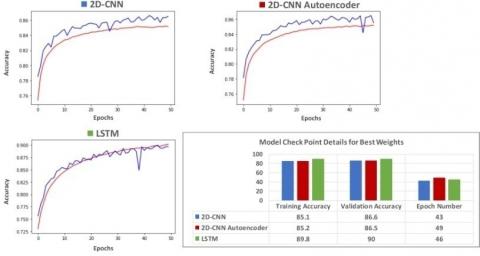
For each model, Adam and sparse categorical cross entropy were selected as optimization and loss function accordingly. The Adam optimizer was configured with default values; and all models were set to fit for 50 epochs. In order to minimize over fitting, model check point was configured to save best weights using validation accuracy as monitor for individual model. All the deep learning models were trained with a batch size of 32. Figure 3 shows the training details at which best weights are saved for each model, and displays the training and validation accuracy curves for the deep learning models.
Figure 3. Learning curves and details of deep models
An accuracy curve for a deep learning model illustrates changes in value of accuracy of the model as it is trained for successive epochs. In Figure 3, for every model, the training accuracy curves are represented in red, while the validation accuracy curves are represented in blue. The initial training accuracies for 2D-CNN and 2D-CNN Autoencoder models were approximately 75%, while initial validation accuracies were approximately 78%. As both models were trained for consecutive epochs, a steady raise in the training and validation accuracies were witnessed until it reached 35th epochs after which the training and validation accuracies hover around 85% and 86% respectively. This signifies that training the models for more epochs will not improve models’ performance.
As for the LSTM model, the training and validation accuracies at the first epochs were approximately 73% and 75%; and both accuracies kept on increasing till the 50th epoch. This suggests that there is tendency for the LSTM model’s performance to improve beyond 90% validation accuracy if it is trained for more epochs. All the three deep learning models did not experience over fitting as validation accuracies were higher than the training accuracies.
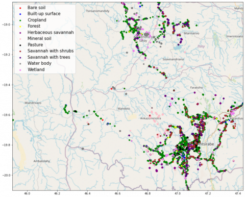
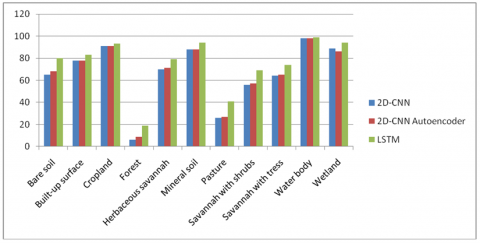
We included F1-score, along with accuracy, for the evaluation of resulting models’ performance on the test set, as the latter only reflects model performance of predominant class in a situation of class imbalance. F1-score is a hybrid metric of recall (producer’s accuracy) and precision (user’s accuracy) which are classed based evaluation metrics that measure how well a model classifies LULC labels in real life, and how real a classified map is on the ground respectively. F1-score facilitate ease of evaluating class based performances of models as it presents a representation of model performance for instances occurrences are affirmed and denounced as single metric. The LSTM model exhibited the best performance for LULC classes’ discrimination on the test set, followed by 2D-CNN Autoencoder model. The least class discrimination capability was exhibited by 2D-CNN model. Table 4 shows the evaluation result for the models on the test set, while Figure 4 and Figure 5 display the Ground truth LULC map and Classified LULC map for the best performing (LSTM) model on the test set, where points on the maps represent average reflectance values of the Sentinel 2 L1C images. Figure 6 shows F1-scores for the three deep learning models on discriminating each LULC class.
Table 4. Evaluation result on test set
|
Deep Learning Model |
Accuracy (%) |
Precision (%) |
Recall (%) |
F1-Score (%) |
|
2D-CNN |
86 |
83 |
60.6 |
66.5 |
|
2D-CNN Autoencoder |
86 |
82.5 |
61.7 |
67.1 |
|
LSTM |
90 |
85 |
70.4 |
75 |
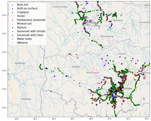
Figure 4. Test set ground truth LULC map showing the distribution of mean reflectance values for Sentinel 2 L1C images of Antsirabe site in Madagascar
Figure 5. LSTM classified LULC map showing the distribution of mean reflectance values for Sentinel 2 L1C images of Antsirabe site in Madagascar
Figure 6. F1-scores for deep learning models per LULC class
In comparison with the reference values, the 2D-CNN and 2D-CNN Autoencoder classifiers correctly predict 83% and 82.25% of land cover types in the test set to belong to classes in which they actually belong respectively; while 60.6% and 61.7% of land cover types in the test set are correctly represented on the classified map generated from the former and latter models correspondingly. The relatively low producer’s accuracies exhibited by the two models are responsible for a satisfactory classification performances of 2D-CNN and 2D-CNN Autoencoder classifiers at 66.5% and 67.1% F1-score (an harmonic mean of user’s and producer’s accuracy) respectively.
On the other hand, the LSTM model adequately classifies 85% of land cover types in the test set to classes they actually belong in the reference values; however, 70.4% of land cover types in the test set are correctly represented on the classified map produced from the LSTM model. The relatively high producer’s accuracy exhibited by the LSTM classifier resulted to improved F1-score of 75% by the model, though still rated satisfactory.
Figure 6 illustrate F1-scores for Deep Learning Models per LULC Class, where the models have the highest F1-scores on discriminating water body class, while the least F1-scores for models were witnessed on Forest class at a maximum F1-score of 19% by LSTM model. A comparison view of Figure 4 and 5 reveals conspicuous misclassifications of the LSTM classifier for forest and pasture classes, with obscure misclassifications for other classes. This implies that the best performing model, in this study, is less suitable for applications where forest and pasture class discriminations are pivotal. All models exhibited good discrimination ability for wetland and mineral soil classes at F1-scores not less than 86%. The exceptional and fair performance of all models on discriminating water body and wetland classes respectively, suggests the suitability of the models for monitoring water boundaries. As for cropland class discrimination, all models exhibited outstanding F1-scores (91% for both 2D-CNN and 2D-CNN Autoencoder, and 93% for LSTM), making them suitable in handling upper layer classification task for crop mapping applications.
In this study, we exploited the JECAM ground truth database to create a Sentinel 2 L1C raster dataset for Antsirabe site with imbalance LULC classes. The entire 13 bands of the satellite dataset were used to build three deep learning models which are 2D-CNN, 2D-CNN Autoencoder and LSTM models. Despite the 2D-CNN model exhibited slightly higher validation accuracy than the 2D-CNN Autoencoder model, the latter has better ability to discriminate between LULC classes. This implies that autoencoding structure for convolution neural methods renders better performances than legacy CNN architecture. The best LULC class discrimination is exhibited by LSTM model at a test accuracy and F1-score of 90% and 75% respectively. This confirms the JECAM database as a fairly suitable ground truth data source for agricultural LULC mapping, which can not only be used for effective land management and mitigating threats to biodiversity, but also can used as a bases to isolate crop image samples as inputs to crop type classifiers to produce crop maps which are essential for innovative crop management strategies such as yield estimation and weed control.
The authors could not access a workstation with adequate GPU (Graphic Processing Unit) and memory to handle computer vision task related to satellite imagery in the context of LULC classification. This pushed the authors to employ Google Colab platform for data modeling in this study. Nevertheless, the mostly available (free) plan offers by Google only allow users to access Colab platform for limited period of time with the exception of the paid plan(s) that is not accessible to users outside the United State of America. The implication of this is that model must be trained for restricted period of time, preventing deep learning models developed in this study to be set to train for a maximum number of 50 epochs. Moreover, this limitation inhibited the authors to adopt state of the art modeling techniques (such as transfer learning, spectral indices, deeper neural network and so on) that can outstandingly improve the discrimination capabilities of deep learning models to produce excellent LULC maps, as these modeling methods potentially require more training time per epoch. In the future, we intend to employ spectral indices and transfer learning to address the problem of class imbalance inherent in the satellite imagery dataset. This, we believe, can improve LULC class discrimination capabilities for resulting models.
[1] Michel, W. (2017). Food insecurity. Animal Agriculture & Sustainable Develop, Knowledge Base. https://kb.wisc.edu/dairynutrient/472ASD/page.php?id=70420, accessed on Jan. 17, 2022.
[2] Poggio, T., Liao, Q. (2018). Theory I: Deep networks and the curse of dimensionality. Bulletin of the Polish Academy of Sciences: Technical Sciences, 66(6): 761-773. https://doi.org/10.24425/bpas.2018.125924
[3] Kussul, N., Lavreniuk, M., Skakun, S., Shelestov, A. (2017). Deep learning classification of land cover and crop types using remote sensing data. IEEE Geoscience and Remote Sensing Letters, 14(5): 778-782. https://doi.org/10.1109/LGRS.2017.2681128
[4] Mazzia, V., Khaliq, A., Chiaberge, M. (2019). Improvement in land cover and crop classification based on temporal features learning from Sentinel-2 data using recurrent-convolutional neural network (R-CNN). Applied Sciences, 10(1): 238. https://doi.org/10.3390/app10010238
[5] Rana, S. Applications of machine learning in common agricultural policy at the rural payments agency. Rural Payments Agency. https://datasciencecampus.ons.gov.uk/wp-content/uploads/sites/10/2019/03/Using_Deep_Learning_for_automatic_identification_of_non-agricultural_land_covers_January2019.pdf
[6] Rußwurm, M., Pelletier, C., Zollner, M., Lefèvre, S., Körner, M. (2019). Breizhcrops: A time series dataset for crop type mapping. arXiv preprint arXiv:1905.11893. https://doi.org/10.48550/arXiv.1905.11893
[7] Sidike, P., Sagan, V., Maimaitijiang, M., Maimaitiyiming, M., Shakoor, N., Burken, J., Mockler, T., Fritschi, F.B. (2019). dPEN: Deep progressively expanded network for mapping heterogeneous agricultural landscape using WorldView-3 satellite imagery. Remote Sensing of Environment, 221: 756-772. https://doi.org/10.1016/j.rse.2018.11.031
[8] Xie, B., Zhang, H.K., Xue, J. (2019). Deep convolutional neural network for mapping smallholder agriculture using high spatial resolution satellite image. Sensors, 19(10): 2398. https://doi.org/10.3390/s19102398
[9] Jolivot, A., Lebourgeois, V., Leroux, L., Ameline, M., Andriamanga, V., Bellón, B., Castets, M., Crespin-Boucaud, A., Defourny, P., Diaz, S., Dieye, M., Dupuy, S., Ferraz, R., Gaetano, R., Gely, M., Jahel, C., Kabore, B., Lelong, C., Maire, G., Seen, D.L., Muthoni, M., Ndao, B., Newby, T., De Oliveira Santos, C.L.M., Rasoamalala, E., Simoes, M., Thiaw, I., Timmermans, A., Tran, A., Bégué, A. (2021). Harmonized in situ datasets for agricultural land use mapping and monitoring in tropical countries. Earth System Science Data, 13(12): 5951-5967. https://doi.org/10.5194/essd-13-5951-2021
[10] Tsendbazar, N.E., De Bruin, S., Herold, M. (2015). Assessing global land cover reference datasets for different user communities. ISPRS Journal of Photogrammetry and Remote Sensing, 103: 93-114. https://doi.org/10.1016/j.isprsjprs.2014.02.008
[11] Fritz, S., See, L., Perger, C., McCallum, I., Schill, C., Schepaschenko, D., Duerauer, M., Karner, M., Dresel, C., Laso-Bayas, J.C., Lesiv , M., Moorthy, I., Salk, C.F., Danylo, O., Sturn, T., Albrecht, F., You, L.Z., Kraxner, F., Obersteiner, M. (2017). A global dataset of crowdsourced land cover and land use reference data. Scientific Data, 4(1): 1-8. https://doi.org/10.1038/sdata.2017.75
[12] Laso Bayas, J., Lesiv, M., Waldner, F., et al. (2017). A global reference database of crowdsourced cropland data collected using the Geo-Wiki platform. Sci Data, 4(1): 170136. https://doi.org/10.1038/sdata.2017.136
[13] Waldner, F., Fritz, S., Di Gregorio, A., Defourny, P. (2015). Mapping priorities to focus cropland mapping activities: Fitness assessment of existing global, regional and national cropland maps. Remote Sensing, 7(6): 7959-7986. https://doi.org/10.3390/rs70607959
[14] Fritz, S., See, L., McCallum, I., You, L.Z., Bun, A., Moltchanova, E., Duerauer, M., Albrecht, F., Schill, C., Perger, C., Havlik, P., Mosnier, A., Thornton, P., Wood-Sichra, U., Herrero, M., Becker-Reshef, I., Justice, C., Hansen, M., Gong, P., Aziz, S.A., Cipriani, A., Cumani, R., Cecchi, G., Conchedda, G., Ferreira, S., Gomez, A., Haffani, M., Kayitakire, F., Malanding, J., Mueller, R., Newby, T., Nonguierma, A., Olusegun, A., Ortner, S., Rajak, D.R., Rocha, J., Schepaschenko, D., Schepaschenko, M., Terekhov, A., Tiangwa, A., Vancutsem, C., Vintrou, E., Wu, W.B., van der Velde, M., Dunwoody, A., Kraxner, F., Obersteiner, M. (2015). Mapping global cropland and field size. Global change biology, 21(5): 1980-1992. https://doi.org/10.1111/gcb.12838
[15] Macrotrends LLC, “Antsirabe, Madagascar Metro Area Population 1950-2022,” 2022. https://www.macrotrends.net/cities/21793/antsirabe/population.
[16] Debie, E., Shafi, K. (2019). Implications of the curse of dimensionality for supervised learning classifier systems: theoretical and empirical analyses. Pattern Analysis and Applications, 22: 519-536. https://doi.org/10.1007/s10044-017-0649-0
[17] Sarker, I.H. (2021). Deep learning: A comprehensive overview on techniques, taxonomy, applications and research directions. SN Computer Science, 2(420). https://doi.org/10.1007/s42979-021-00815-1
[18] Scherer, D., Müller, A., Behnke, S. (2010). Evaluation of pooling operations in convolutional architectures for object recognition. In Artificial Neural Networks–ICANN 2010: 20th International Conference, Proceedings, Springer Berlin Heidelberg, 92-101. https://doi.org/10.1007/978-3-642-15825-4_10
[19] Bezdan, T., Bačanin Džakula, N. (2019). Convolutional neural network layers and architectures. In Sinteza 2019-International Scientific Conference on Information Technology and Data Related Research, Singidunum University, 445-451. https://doi.org/10.15308/Sinteza-2019-445-451
[20] Ghosh, A., Sufian, A., Sultana, F., Chakrabarti, A., De, D. (2020). Fundamental concepts of convolutional neural network. Recent Trends and Advances in Artificial Intelligence and Internet of Things, 519-567. https://doi.org/10.1007/978-3-030-32644-9_36
[21] Gholamalinezhad, H., Khosravi, H. (2020). Pooling methods in deep neural networks, a review. arXiv preprint arXiv:2009.07485. https://doi.org/10.48550/arXiv.2009.07485
[22] Basha, S.H.S., Dubey, S.R., Pulabaigari, V., Mukherjee, S. (2020). Impact of fully connected layers on performance of convolutional neural networks for image classification. Neurocomputing, 378(22): 112-119. https://doi.org/10.1016/j.neucom.2019.10.008
[23] Hochreiter, S. (1991). Untersuchungen zu dynamischen neuronalen Netzen. Diploma, Technische Universität München, 91(1).
[24] Elman, J.L. (1990). Finding structure in time. Cognitive science, 14(2): 179-211. https://doi.org/10.1207/s15516709cog1402_1
[25] Rumelhart, D.E., Hinton, G.E., Williams, R.J. (1986). Learning representations by back-propagating errors. Nature, 323(6088): 533-536. https://doi.org/10.1038/323533a0
[26] Pascanu, R., Mikolov, T., Bengio, Y. (2013). On the difficulty of training recurrent neural networks. In International Conference on Machine Learning, Pmlr, 1310-1318.
[27] Bengio, Y., Simard, P., Frasconi, P. (1994). Learning long-term dependencies with gradient descent is difficult. IEEE Transactions on Neural Networks, 5(2): 157-166. https://doi.org/10.1109/72.279181
[28] Graves, A., Liwicki, M., Fernández, S., Bertolami, R., Bunke, H., Schmidhuber, J. (2008). A novel connectionist system for unconstrained handwriting recognition. IEEE Transactions on Pattern Analysis and Machine Intelligence, 31(5): 855-868. https://doi.org/10.1109/TPAMI.2008.137
[29] Hochreiter, S., Schmidhuber, J. (1997). Lonf short-term memory. Neural Computation, 9(8): 1735-1780. https://doi.org/10.1162/neco.1997.9.8.1735
[30] Greff, K., Srivastava, R.K., Koutník, J., Steunebrink, B.R., Schmidhuber, J. (2016). LSTM: A search space odyssey. IEEE Transactions on Neural Networks and Learning Systems, 28(10): 2222-2232. https://doi.org/10.1109/TNNLS.2016.2582924
[31] Chollet, F. (2016). Building autoencoders in keras. The Keras Blog, 14. https://blog.keras.io/building-autoencoders-in-keras.html
[32] Sewani, H., Kashef, R. (2020). An autoencoder-based deep learning classifier for efficient diagnosis of autism. Children, 7(10): 182. https://doi.org/10.3390/children7100182
[33] Zhu, Q.Y., Zhang, R.X. (2019). A classification supervised auto-encoder based on predefined evenly-distributed class centroids. arXiv preprint arXiv:1902.00220. https://doi.org/10.48550/arXiv.1902.00220