Hasan Polat
© 2022 IIETA. This article is published by IIETA and is licensed under the CC BY 4.0 license (http://creativecommons.org/licenses/by/4.0/).
OPEN ACCESS
Alzheimer’s disease (AD) is a neurodegenerative disorder with an unknown etiology and a significant prevalence. Rapid and accurate detection of AD is crucial to assist in a more effective and tailored treatment plan to delay the progression of the disease. This paper introduces a novel approach based on a time-frequency complexity map (complextrogram) for the automated AD diagnosis. The complextrogram is the topographic complexity level of an EEG signal, plotted as a function of time and frequency. The complextrogram representations were fed into a well-known lightweight deep neural network called MobileNet for robust performance on resource and accuracy tradeoffs. The experiments were performed using a five-fold cross-validation technique on a publicly available database containing clinical EEG recordings from 24 patients with AD and 24 healthy, age-matched controls. The proposed pipeline provided competitive performance with just 2.2 M parameters and achieved the best overall accuracy for some locations in the frontal lobes (Fp2 and F8 channels). For both channels, the classification accuracy was 100%. Also, the violin plot was used to get further details of the distribution of complexity values for specific frequency rhythms. After statistical evaluation, it was observed that neurodegenerative conditions caused changes in chaotic behaviors, including increased delta complexity and decreased alpha complexity. Results demonstrated that the complextrogram representation proved its potency for the input quality required by the deep learning architectures. Furthermore, the complextrogram method is a promising pathway to discriminate and reflect the fundamental characteristics of AD abnormalities.
Alzheimer’ disease, EEG, deep learning, entropy, MobileNet, complexity
Alzheimer’s disease (AD) is one of the most common forms of dementia [1, 2]. AD is a progressive neurodegenerative disorder with an unknown etiology and a significant prevalence [3]. This disorder leads to severe symptoms such as memory loss and cognitive decline. It thus negatively affects the basic activities of daily living [4]. Rapid and accurate detection of AD can contribute significantly to reducing its destructive effect.
AD is diagnosed through neuropsychological assessments that require long experimental sessions and experienced professionals. The fact that the pathophysiological mechanism at the basis of AD is still not fully understood makes the early and accurate diagnosis of the disease very difficult [5]. Neuroimaging techniques such as functional magnetic resonance imaging (fMRI), positron emission tomography (PET), computed tomography (CT), and electroencephalography (EEG) have a great potential to assist clinicians [6, 7]. Compared to other imaging tools, EEG is one of the most popular techniques in AD research due to its high temporal resolution, non-invasiveness, and relatively low financial cost [8]. EEG can effectively reflect the brain dynamics of neurodegenerative diseases. It has the capability of an alternative validation test for AD diagnosis. Slowed oscillations, decreased coherence, and drastic changes in subband power in EEG signals are the most typical traits observed with AD [9]. However, visually analyzing disease-specific brain dynamics from EEG signals is a challenging task and is error-prone [10]. The development of an automated EEG-based diagnostic system is critical to initiating treatment that can significantly delay disease progression, potentially leading to improved patient quality of life and reduced healthcare costs.
Machine learning-based AD diagnosis from EEG has become a critical approach to assist traditional visual inspection-based techniques. Conventional classifier architectures such as support vector machine (SVM), naïve Bayes (NB), random forest (RF), k-nearest neighbors (KNN), and linear/quadratic discriminant analysis (LDA/QDA) can successfully classify disease-specific EEG features [3, 11, 12]. Since hand-crafted features directly affect the classifier performance, it is crucial to determine proper feature extraction methods. The effectiveness of hand-crafted features often requires assumptions such as stationarity, high time or frequency resolution, and a high signal-to-noise ratio [9]. In this context, various linear and nonlinear features have been frequently used for AD diagnosis, such as amplitude envelop and spectral analysis [13, 14], Hurst exponent measures [15], relative band power [16], permutation entropy [17, 18], spectral entropy [19], fuzzy entropy [20], wavelet parameters [21], cross-correlation coefficients [22]. A robust feature extraction process is usually accomplished by experience or trial and error. This strategy may not settle well for such a complicated task [7]. Also, designing a robust conventional pipeline requires a lot of effort and is time-consuming.
Deep learning (DL), one of the machine learning techniques, has shown impressive performance in several classification tasks without feature engineering [23, 24]. DL does not require hand-crafted features and can extract features directly from raw data automatically [23]. This ability has attracted enormous interest from researchers due to its impressive performance in pattern recognition. However, one of the most crucial factors affecting DL performance is how inputs have been fed. Because DL models have a great potential in image processing, EEG time series usually are represented in image format (2D or 3D). In order to potentially improve DL performance, EEG data are represented as time × channel matrices [25], time-frequency representation such as spectrogram [26] or scalogram [27].
The prevalence of DL-based systems in the biomedical field has increased, with the recent development of graphics processing units (GPUs) providing an inexpensive and robust solution to hardware bottlenecks [8]. Previous works proposed efficient AD diagnosis pipelines based on various input formulations and deep network designs. Morabito et al. [28] employed the convolutional neural network (CNN) model to explore the representation power of DL in automated feature extraction. The proposed model enforced a series of convolutional subsampling layers to derive a novel pattern in the classification task of the prodromal version of dementia. Bi and Wang [7] proposed a multi-task learning strategy based on a convolutional high-order Boltzmann Machine for early AD diagnosis. The proposed DL pipeline could extract more abstract features from EEG spectral images. As a result, the high-level representations provided superior performance over several state-of-the-art methods. Rodrigues et al. [10] introduced an automated AD diagnosis model using an EEG-based deep learning framework. In order to improve the performance of the DL network, EEG signals were represented as matrices of connections utilizing the various causality and correlations measures. Ismail et al. [29] converted EEG subbands into RGB image form for CNN-based early AD diagnosis by considering channel locations. Their strategy of handling EEG data as a video allowed training CNN for video classification. Huggins et al. [27] used resting-state scalp EEG signals to perform a multi-classification task. In order to boost DL performance, EEG data were represented as time-frequency graphs (scalogram) using continuous wavelet transform. They employed an AlexNet on scalogram images to contribute diagnosis of AD.
This paper introduces a novel approach based on a time-frequency complexity map (complextrogram) of EEG signals to boost AD diagnosis performance. The term complextrogram was defined, inspired by the scalogram and spectrogram methods. The complextrogram is the entropic complexity level of an EEG signal, plotted as a function of time and frequency. Entropy analysis is performed as the essential function of the complextrogram method, as it is a robust technique to evaluate the unpredictability or complexity level of the time series. The complextrogram explores the phenomena of varying complexity for each frequency component during the period in which the signal is observed. More specifically, it creates new patterns as a function of time and frequency, considered robust multidimensional representations. Thus, alternations of the chaotic structure of brain activities in the time and frequency axis are represented topographically. AD diagnosis is performed from complextrogran images reflecting nonlinear features of EEG signals by employing a well-known lightweight deep neural network, called MobileNet [30, 31]. The primary contributions of this study are as follows:
1. This paper presents the complextrogram method, which is a novel representation of EEG signal. Since the performance of the DL highly depends on input quality, input formulization is crucial for the robust representation. In this context, the complextrogram approach has a great potential to design a robust DL pipeline in the diagnosis of neurodegenerative disorders from EEG signals.
2. The proposed DL pipeline was performed separately for the 19 available EEG channels. Channel-specific analyses may point out cerebral cortex areas where AD anomalies appear most prominently. Moreover, it will provide a crucial pathway for researchers to determine distinctive channels associated with complexity-type EEG patterns.
3. The majority of current deep neural network-based diagnosis approaches are not suited for clinical usage due to hardware implementation requirements. This study proposes a lightweight DL architecture for AD diagnosis. The idea of a lightweight model can offer the opportunity to design more suitable for on-device various diagnosis applications.
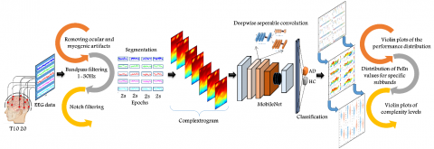
The proposed AD diagnosis system consists of a complextrogram representation-based DL framework. Figure 1 graphically depicts the overall pipeline, including data acquisition, preprocessing steps, obtaining complextogram representations, the proposed lightweight DL model, and statistical analysis. This section presents details of each part included in the proposed pipeline.
Figure 1. An illustration of the proposed methodology for automated AD diagnosis based on complextrogram representation
2.1 EEG data acquisition
The AD database considered here was created jointly by researchers at Florida State University [9]. The EEG data were collected at a sampling frequency of 128 Hz and a duration of eight seconds for each individual and from 19 scalp electrodes (Fp1, Fp2, F7, F3, Fz, F4, F8, T3, C3, Cz, C4, T4, T5, P3, Pz, P4, T6, O1, and O2) based on the international 10-20 system. The letter labels F, C, P, O, and T refer to, parietal frontal, central, occipital, and temporal cerebral lobes, respectively. EEG recordings which include two subject groups, AD patients and healthy controls (HC), were collected under two resting-states, eyes open by visual fixation and eyes closed. Subsequently, both groups were divided into sub-groups according to eyes open (A and C) and closed (B and D). Groups A and B represent HC that consist of 24 healthy elderly participants (average age 72 ± 11 years) with no personal history of neurological disorders. The two other groups (C and D) comprise 24 probable AD patients (average age of 69 ± 16 years) diagnosed according to the National Institute of Neurological and Communicative Disorders and Stroke, the Alzheimer's Disease and Related Disorders Association (NINCDS-ADRDA), following the Diagnostic and Statistical Manual of Mental Disorders (DSM)-III-R criteria. Figure 2 illustrates exemplary EEG signals for each group.
2.2 EEG preprocessing
The raw EEG recordings are naturally susceptible to contamination with various structural forms. The artifacts typically occur in several types that come from different sources such as ocular, cardiac, muscle, electrical interference, and electrode displacement [32]. Preprocessing techniques are not only for AD diagnosis but are common to almost all neuroscience tasks [33]. The preprocessing strategy generally consists of three steps; artifacts suppression, filtering of EEG signals to obtain specific bandwidths, and segmentation process for short-time EEG epochs [23, 32, 33].
The EEG data used in this study was recorded free from ocular and myogenic artifacts. In order to remove power grid interference, a notch filter was applied. Since EEG recordings are band-limited to the range of 1-30 Hz, no specific band-pass filter was applied. EEG signals were segmented into 2 s epochs with no overlap. The epoch length is the most commonly used period length in AD research [33]. Thus, analysis of cleaner EEG recordings was achievable to avoid potential errors in the complextrogram representation.
2.3 Complextrogram theory for input formulation
Complextrogram is a topographic representation that demonstrates changes in complexity characteristic of an EEG signal as a function of time and frequency. It can provide valuable details for alternations of the chaotic structure of brain activities. In this context, entropy analysis is employed as the essential function. Entropy is one of the most commonly used nonlinear techniques in evaluating the chaotic characteristics of time series. It is a robust biomarker to reflect EEG complexity for monitoring brain abnormalities [1, 34, 35]. The hypothesis of decreasing the chaotic behavior of brain activity during AD can be quantified by using the entropy approach [36].
There are many rigorous and widespread entropy metrics for complexity analysis, such as approximate entropy (ApEn), sample entropy (SampEn), Renyi entropy (ReEn), permutation entropy (PeEn), Tsallis entropy (TsEn), and spectral entropy (SpecEn). In this study, the PeEn method was used for complextrogram due to its relative simplicity, low complexity in computation, and robustness in short and noisy observations [1, 36]. The proposed complextrogram technique utilizes PeEn but is not limited.
Figure 2. Exemplary EEG segments for channel F8 (The columns are healthy controls and patients with AD, respectively. The rows represent resting-state paradigms, eyes open and eyes closed, respectively.)
2.3.1 Permutation entropy
The mathematical definition of the PeEn theory was presented in detail in Refs. [35-38]. The complexity level for an EEG epoch in terms of PeEn metric can be estimated as follows:
1. If an EEG time series consisting of N data points is expressed as x(i)=[x1, x2, x3, …. xN], xi indicates to ith sample of the EEG signal.
2. The signal can be reconstructed from subsets type using embedded size (m) and time delay (τ) as $X_1=\left[x_1, x_{1+\tau}, \ldots, x_{1+(m-1) \tau}\right], \ldots, X_i\left[x_i, x_{i+\tau}, \ldots x_{i+(m-1) \tau}\right], \ldots, X_{N-(m-1) \tau}=\left[x_{N-(m-1) \tau}, x_{N-(m-2) \tau}, \ldots x_N\right]$. Here, the m number of real values contained in each Xi can be arranged in increasing order as $\left\{x_{\left(i+\left(j_1-1\right) \tau\right)} \leq x_{\left(i+\left(j_2-1\right) \tau\right)} \leq \cdots \leq x_{\left(i+\left(j_m-1\right) \tau\right)}\right.$. If there are two or more elements of the same value in Xi, their original positions can be sorted such that for $j_1 \leq j_2 x_{\left(i+\left(j_1-1\right) \tau\right)} \leq x_{\left(i+\left(j_2-1\right) \tau\right)}$. Thus, we can map any vector x(i) onto a set of symbols. If a set of symbols is expressed as:
$s(l)=\left(j_1, j_2, j_3, \ldots j_m\right)$ (1)
where, l=1, 2, 3, …, k and k≤m! (m! is the largest number of distinct symbols). s(l) is one of the m! symbol permutations, which is mapped onto the number symbols (j1, j2, j3, … jm) in m-dimensional embedding space.
3. If P1, P2, P3, … Pk denote the probability distribution of each symbol sequence, respectively. The PeEn of order m for the can be formulated as:
$H_{P E}(m)=-\sum_l^k P_1 \ln P_1$ (2)
The permutation entropy of order m can be normalized as:
$0 \leq H_{P E}(m)=H_{P E}(m) / \ln (m !) \leq 1$ (3)
When the maximum value of PeEn is equal to ln(m!), this means that all the symbol sequences have equal probability. In contrast, the smallest value of PeEn denotes that the time series is very regular. For a robust complexity analysis, various applications have frequently selected embedded dimension m=3, 4, …, 7. The time delay factor is performed as 1 to take successive points into the calculation.
2.3.2 The complextrogram matrix
The steps for obtaining the complextrogram representations are as follows:
1. EEG epochs are bandpass filtered between fn to fn+1 Hz using the 4th order Butterworth filter. The frequency range fn and fn+1 is the initial frequency for complextrogram representation. To remove significant power at low frequencies (~0 Hz) caused by the DC offset, fn=0.5 Hz or a higher frequency will be suitable.
2. A rectangular window with a particular window size W=n and n $\in$ [1, N] is continuously shifted on the signal along the time axis. Here, n is the window length, and N is the length of the discrete-time source signal $x(i)=\left[x_1, x_2, x_3, \ldots . x_N\right]$.
3. For each signal sequence where the window overlaps $\left(x(i) \cap W_n\right)$, the PeEn metric $P e_{\left(x(i) \cap W_n\right)}$ is calculated.
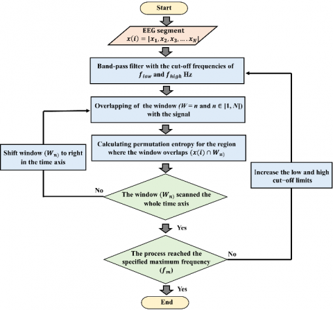
4. The low and high cutoff limits of the band pass filter are incrementally increased. Steps 1, 2 and 3 are repeated for all the time intervals until the process reaches the specified maximum frequency (fm). In order to determine the maximum frequency, the Nyquist criterion (fs≥2fm) will be suitable if no low pass or band pass filter is applied in the preprocessing stage. Here, fs denotes the sampling frequency. Figure 3 illustrates the flow chart of the methodologies applied for the proposed complextogram representation.
After the processing steps aforementioned, the complextrogram matrix can be constructed as:
$\operatorname{Comp}(X)=\left[\begin{array}{cccc}C_{1,1} & C_{1,2} & \ldots & C_{1, j} \\ C_{2,1} & C_{2,2} & \ldots & C_{2, j} \\ \vdots & \vdots & \ddots & \vdots \\ C_{i, 1} & C_{i, 2} & \ldots & C_{i, j}\end{array}\right]$ (4)
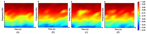
For an Ci,j element of the matrix, i and j denote spatial position that includes time and frequency information, respectively. C denotes the level of complexity of the EEG signal at that location. For the complextrogram representation, embedding dimension m of 3 and time delay τ of 1 were found suitable for the PeEn metric. The window size was set to 32, the initial frequency to 1Hz, and the maximum frequency to 30Hz. Figure 4 shows topographic visualizations of complextrogram matrices of sample EEG signals from AD patients and healthy participants.
Figure 3. The flow chart of the procedures applied for the proposed complextogram representation
Figure 4. Complextrogram representations of sample EEG signals from each of the four groups. (a) and (b) are HC in the resting state with eyes open and closed, respectively. (c) and (d) are patients with AD, eyes open and closed, respectively. The colorbar represents the EEG complexity levels
2.4 Mobilenet for a lightweight deep learning model
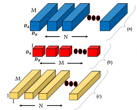
Howard et al. proposed an efficient network architecture called MobileNets for robust performance on resource and accuracy tradeoffs [30]. The MobileNet framework employs depthwise separable convolutions for less computation than standard convolutions. The hypothesis of depthwise separable convolution is to factorize a standard convolution into depthwise and pointwise convolution. This factorization causes drastically accelerating the computation and reducing the model size. Figure 5 illustrates a depthwise separable convolution operation.
For a square input, the standard convolutional layer uses the input as a DF×DF×M feature map (F). DF denotes the spatial width and height of the input, and M is the input depth. It then produces an output feature map (G) with the size of DF×DF×N, where DF denotes the spatial width and height of the output, and N is the output depth. The number of learnable parameters in the standard convolution layer is determined by the convolution kernel (K) of size DK×DK×M×N that assumed a square. Consequently, the learnable parameter size of standard convolutions is computed as:
$D_K \cdot D_K \cdot M \cdot N \cdot D_F \cdot D_F$ (5)
The number of input channels M, the number of output channels N, the kernel size DK×DK and the feature map size DF×DF directly affect the computational cost. The direct interaction of the parameters causes the computational cost to increase exponentially. Therefore, breaking the interaction can prevent the exponential increase. MobileNet can break direct interaction by splitting standard convolutional filter into two layer. It uses depthwise convolutions to apply a single filter per each input channel. First, it uses depthwise convolutions to apply a single filter per each input channel. For depthwise convolution, the computational cost is defined as:
$D_K \cdot D_K \cdot M \cdot D_F \cdot D_F$ (6)
In order to create a linear combination of the output of the depthwise layer, pointwise convolution, a simple 1×1 convolution, is then used. The final computation cost at the end of the two layers is as:
$D_K \cdot D_K \cdot M \cdot D_F \cdot D_F+M \cdot N \cdot D_F \cdot D_F$ (7)
As a result, the deeply separable convolution operation reduces the computational cost by almost 9 times compared to standard convolution. MobileNets employ both batchnorm and ReLU nonlinearities for each convolutional step.
In this study, the MobileNetV2 model, which is a variant of the MobileNet architecture, was used. The main novelty of this variant is the inverted residual with linear bottleneck [31]. This update has reduced the computational cost of the original framework by about 2.5 times.
Figure 5. The factorization of a standard convolutional filter (a) into two layers. (b): depthwise convolutional filter, (c): pointwise convolutional filter
2.5 Hyperparamater tunning
The proposed DL-based diagnosis framework uses a lightweight convolutional network called MobileNet that typically has millions of parameters. The MobileNet structure is designed on depth separable convolutions, except for the first layer, which is a full convolution [30]. Its network topology is crucial for making robust solutions. MobileNets use both batch normalization and ReLU activation for both separate layers. Batch normalization can reduce the computation time of the DL pipeline by shifting input samples. Since it revises the inputs to have unit variance and zero mean at each mini-batch, it causes a tremendous difference in improving the training time and accuracy [39, 40]. The ReLU solves the vanishing gradient problem for training deep learning approaches.
For the optimization, the ADAM optimizer is used in the training network since it has a fast convergence rate [41]. The initial learning rate was set as 0.001 and then decreased by a rate of 0.4 after every 4 epochs so that the network does not get stuck at the local minimum. Classification task was performed with batch size of 32 for 10 epochs. In order to minimize the risk of overfitting, the early stopping method was kept active.
2.6 Implementation and evaluation
The proposed lightweight pipeline was performed separately for the 19 available EEG channels. As a result of segmentation for 2 s with no overlap, 192 EEG segments from healthy elderly control subjects and AD patients were obtained for each channel. A total of 3648 complextrogram images were used for all channels. The dataset consisting of 192 images for each channel is divided into three sets for training, validation, and testing, with proportions of 0.60, 0.20, and 0.20, respectively. In addition, a five-fold cross-validation technique was applied to partition the dataset to ensure reliable generalization.
The selection of appropriate model evaluation metrics is a crucial issue to provide further insights on the influence of the complexrogram representation in AD diagnosis. The ideal metric should heavily focus on the classifier's ability to identify patterns belonging to different groups. In this context, accuracy, sensitivity, specificity, precision, and F1-score metric are favorable because they are reliable indicators for classification performance. All of these metrics can be calculated as:
Accuracy $=\frac{T P+T N}{T P+F P+T N+F N}$ (8)
Sensitivity $($ Recall $)=\frac{T P}{T P+F N}$ (9)
Specificity $=\frac{T N}{T N+F P}$ (10)
Precision $=\frac{T P}{T P+T N}$ (11)
$F 1-$ score $=2 \times \frac{\text { Precision } \times \text { Recall }}{\text { Precision }+\text { Recall }}$ (12)
For the binary classification, TP, FP, TN, and FN denote the true positive, false positive, true negative, and false negative rate, respectively.
The receiver operating characteristic (ROC) curve was also employed as another performance metric. It can demonstrate the relation between the rate of true positives and false positives. The area below this curve, called the area under the ROC curve (AUC), has been widely used in various classification problems [10].
The sequential steps, such as EEG preprocessing, creation of the complextrogram representations, and the application of MobileNet, a lightweight deep learning model, were implemented in the Matlab (The MathWorks, Natick, MA, USA) environment. The experiments were conducted on a 2.7-GHz Intel dual-core i7 processor with 16 GB RAM, NVIDIA GeForce ROG-STRIX 256 bit, and 8GB GPU hardware.
3.1 Channel-specific discrimination of patients with ad from healthy controls
The proposed DL pipeline was performed separately for the 19 available EEG channels. This strategy can also demonstrate the influences of electrode position on the distinction between HC and patients with AD. The complextrogram representation-based classification performance was evaluated in terms of accuracy, specificity, sensitivity, precision, F1-score, and AUC metrics. Table 1 demonstrates the overall classification performance for each EEG channel recorded from resting states, eyes open and closed.
The accuracy metric is the most straightforward and reliable technique to show the ability of the proposed framework in balanced data. The results demonstrated that the classification accuracy for all EEG channels varied, ranging from 48.39% and 100%. The complextrogram-based DL pipeline revealed the best overall performance in some locations in the frontal lobes (Fp2 and F8). The proposed model presented a classification accuracy of 100% for both channels. The temporal lobe channels, excluding the T3, produced high-quality input representations to feed into the lightweight DL model. The proposed model for the T6, T5, and T4 electrode positions achieved an accuracy of 99.47%, 97.89%, and 97.92%, respectively. For other EEG channels, the classifier framework revealed a significantly better accuracy performance for O2, C4, and Pz channels, respectively. These channels presented classification accuracy ranging from 98.42% to 99.47%. After the five-fold cross-validation, the complextrogram verified the remarkable input quality for the DL pipeline.
Table 1. Overall classification performance of each EEG channel with resting states, eyes open and closed
|
% |
Acc. |
Spe. |
Sen. |
Pre. |
F1 |
AUC |
|
Fp1 |
89.07 |
88.68 |
89.47 |
89.24 |
88.94 |
93.21 |
|
Fp2 |
100 |
100 |
100 |
100 |
100 |
100 |
|
F7 |
51.57 |
57.42 |
45.73 |
53.26 |
46.76 |
48.45 |
|
F3 |
83.23 |
82.21 |
84.26 |
84.46 |
83.84 |
92.17 |
|
Fz |
48.39 |
48.89 |
47.89 |
49.87 |
48.13 |
44.19 |
|
F4 |
80.10 |
77.94 |
82.26 |
81.22 |
80.87 |
90.55 |
|
F8 |
100 |
100 |
100 |
100 |
100 |
100 |
|
T3 |
50.97 |
48.89 |
53.05 |
50.99 |
51.58 |
52.01 |
|
C3 |
81.21 |
84.52 |
77.89 |
84.10 |
80.08 |
90.74 |
|
Cz |
86.92 |
88.52 |
85.31 |
89.36 |
86.39 |
94.09 |
|
C4 |
98.42 |
98.94 |
97.89 |
99 |
98.37 |
99.55 |
|
T4 |
97.92 |
96.89 |
98.94 |
97.04 |
97.94 |
100 |
|
T5 |
97.89 |
96.84 |
98.94 |
97 |
97.92 |
99.94 |
|
P3 |
80.21 |
74 |
86.42 |
77.74 |
81.67 |
90.03 |
|
Pz |
98.42 |
97.89 |
98.94 |
98 |
98.43 |
100 |
|
P4 |
80.73 |
81.42 |
80.05 |
83.09 |
79.93 |
89.55 |
|
T6 |
99.47 |
98.94 |
100 |
99 |
99.48 |
99.94 |
|
O1 |
84 |
88.57 |
79.42 |
87.13 |
82.71 |
92.63 |
|
O2 |
99.47 |
100 |
98.94 |
100 |
99.45 |
100 |
Notes: Acc.: Accuracy, Sen.: Sensitivity, Spe.: Specificity, Pre.: Precision, F1: F1-score, AUC: Area under the curve.
Sensitivity and specificity are crucial metrics to evaluate the performance of identifying positive and negative classes, respectively. Table 1 shows that the specificity performance is 100% for the F8, Fp2, and O2 channels, while the sensitivity performance is perfect for the F8, Fp2, and T6 channels. Furthermore, the model obtained a specificity of 98.94% and 97.89% from the T6 and Pz channels, as well as a sensitivity of 98.94% and 97.89% from the O2 and C4 channels for AD diagnosis, respectively. The precision metrics demonstrate whether the correctly classified instances of AD patients are actual AD patients and whether the rest are HC incorrectly labeled as AD. It is s a robust indicator when there is a high cost of having false positives. However, the precision results revealed that the proposed model did not generate false-positive costs. The F1-score represents the average of the precision and recall (sensitivity). Table 1 indicated that f1-score values for all channels are generally close to the accuracy performances. The proposed model presented an f1-score rate of 100% for both Fp2 and F8 channels.
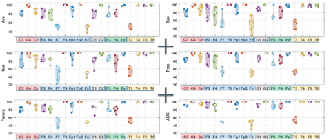
In this study, the violin graph is used to visualize the statistical distributions of performance yielded by each classification fold. Figure 6 illustrates the violin plot of the performance distribution of five-fold cross-validation for each EEG channel.
Figure 6 shows that accuracy performance has low variance in the five-fold cross-validation result, especially for temporal lobe locations, except for the channels where HC and AD classes are perfectly discriminated. For the temporal lobe region, including T4, T5, and T6, the accuracy performance distribution showed a standard deviation ranging from 1.16% to 1.18%. Although some electrodes in frontal lobes revealed the best classification performance, the majority of its channels performed with high variance in different training and testing strategies. The accuracy performance distribution for Fp1, Fz, and F4 showed a standard deviation of 9.35%, 8.79%, and 7.56%, respectively, during the five-fold cross-validation.
Figure 6. Violin plot of the performance distribution of five-fold cross-validation for each EEG channel. (The x-axis represents channel information. Furthermore, each color denotes a different brain lobe, the y-axis represents diagnosis performance by Acc., Sen., Spe., Pre., F1-score, and AUC, respectively.)
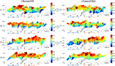
Figure 7. Distribution of PeEn values for specific frequency bands (the x-axis denotes each participant in which participants number 1-24 patients with AD, 25-48 are HC, the y-axis indicates epoch number)
Figure 8. Violin plots of complexity levels for participants belonging to HC and AD groups according to specific subbands (The first and second rows show the plots for the F8 and Fp2 channels, respectively. The first, second, third, and fourth columns show delta, theta, alpha, and beta subbands, respectively.)
Channel-based violin plots indicated a significant increase in variance in the sensitivity and specificity distribution compared to the accuracy performance. For all cerebral lobes, the frontal and parietal regions had the highest variance in specificity performance distribution, respectively. For the frontal lobe region, including Fp1, F7, F3, Fz, and F4 channels, the specificity performance distribution showed a standard deviation ranging from 10.99% to 20.33%. The standard deviation of specificity performances for P3, Pz, and P4 ranged from 2.88% to 14.76%. Compared with the specificity, the sensitivity performance revealed an overall lower variance for all EEG channels. More specifically, sensitivity performances with standard deviations ranged from 2.35% to 11.44% were obtained for the T3, T4, and T5 channels. For the T6 channel, the AD patterns were perfectly discriminated from the healthy controls, and the standard deviation of sensitivity performance was determined as 0.0%. Sensitivity distribution also revealed satisfactory performance for the frontal lobe region, including Fp2 and F8.
3.2 Evaluation of the complexity levels for some specific frequency rhythms
Complextrogram technique revealed that AD dysfunctions could be represented most efficiently in some loci in the frontal and most of the right temporal lobes. Since these local regions offer robust classification performances based on the complextrogram, it is crucial to evaluate their complex behavior. In this context, analyzing complexity level were performed within specific frequency bands, including delta (δ: 0.5–4 Hz), theta (θ: 4–8 Hz), alpha (α: 8 13 Hz), and beta (β: 13–30 Hz). The subband rhythms have proven very efficient in AD diagnosis tasks. Figure 7 illustrates the distribution of PeEn values for specific frequency bands for the frontal regions.
In this study, the violin plot method was also used to get further details of the distribution of PeEn values for specific frequency bands. The violin plots illustrate summary statistics of the overall complexity level for the HC and AD patient groups.
Figure 8 shows that the chaotic dynamics of the EEG vary significantly concerning the subbands. It has been reported that neurodegenerative conditions reduce the unpredictability of alpha oscillations. For AD patients, the mean PeEn values of alpha oscillations from the F8 and Fp2 channels were reported as 0.681 and 0.683, respectively. On the other hand, the mean PeEn values of alpha oscillations from the F8 and Fp2 channels for the HC group were reported as 0.694 and 0.697, respectively. Violin plots related to alpha oscillations show that the complexity levels in both groups were concentrated around the median. The results demonstrate the functional role of alpha oscillations in the complexity analysis of Alzheimer's disease. For beta oscillations, it was determined that the median points were close for both groups, but the PeEn value distributions for AD patients had a higher variance. For AD patients, the standard deviation of the PeEn values is 0.013 and 0.011 for F8 and Fp2, respectively, while the standard deviation of the PeEn values for the HC is 0.009 and 0.018.
The state-of-the-art DL models do not require precisely designed hand-crafted features for a robust diagnosis. Instead, the models automatically learn optimal features from data. Deep learning architectures have successfully applied these capabilities in many EEG-based diagnostic and classification tasks, including AD diagnosis, motor imagery, seizure detection, sleep stage scoring, and emotion recognition tasks. However, the input formulation of the EEG signals directly affects the performance of the proposed models. The input formulation should represent the natural variations of the EEG without ignoring the fundamental characteristics (non-linear and non-stationary) [8, 23, 39]. The successful results obtained in this study showed that the complextrogram method is promising as it is a natural variant of EEG signals and reflects well the fundamental characteristics.
Brain activity contains several EEG rhythms that indirectly reflect the fundamental characteristic of neurodegenerative conditions. Previous studies have emphasized that decreasing complexity, especially at higher frequency rhythms, can be assumed as a potential diagnostic biomarker in AD patients [1, 6, 18]. With this motivation, the variation of the subband complexity dynamics for EEG channels that offered the best classification performance was also explored. After statistical evaluation, it was observed that neurodegenerative conditions caused changes in chaotic behaviors, including increased delta complexity and decreased alpha complexity. The fact that the results are consistent with the literature indicates that the loci in the cerebral lobes determined by the proposed model for AD diagnosis are well-directed.
For evaluation of the efficiency of complextrogram representation, the proposed model was compared to other available conventional and deep learning pipelines based on EEG signals. Further details of the related works considered for the comparison were categorical structured and summarized in Table 2.
Table 2. An overview of the related works to compare the accuracy performance achieved by the proposed pipeline
|
Author(s) |
EEG marker(s) |
Classifier |
Channel |
Epoch length |
Subjects |
Classification problem |
Acc. |
|
Chen et al. [22] |
Detrended cross correlation analysis coefficients |
LDA |
16 |
8 s |
15 AD, 15 HC |
AD/HC |
90% (C3 and P3) |
|
Oltu et al. [16] |
DWT, relative band power, coherence |
Bagged Trees |
19
|
30 s |
8 AD, 16 MCI, 11 HC |
AD/MCI/HC |
96.5% |
|
Deng et al. [17] |
Multivariate multi-scale weighted PeEn |
ROC analysis |
16 |
8 s |
14AD, 14 HC |
AD/HC |
96.7% (right frontal region) |
|
Falk et al. [13] |
HHT, Amplitude modulation analysis |
SVM |
19
|
5 s |
10AD, 11 MCI, 11 HC |
AD/HC |
90.6% |
|
Sharma et al. [19] |
PSD, spectral entropy, fractal dimension |
SVM |
21
|
- |
15AD, 15MCI, 13 HC |
AD/HC |
82% |
|
Babiloni et al. [42] |
Cortical sources of power and functional connectivity |
ROC analysis |
19
|
2 s |
120 AD, 100 HC |
AD/HC |
75.5% |
|
Bi and Wang [7] |
EEG spectral image |
CssCDBM |
64
|
60 s |
4AD, 4MCI, 4HC |
AD/MCI/HC |
95.04% |
|
Morabito et al. [28] |
Time-frequency representation |
CNN |
19
|
5 s |
63AD, 56 MCI, 23 HC |
AD/HC AD/MCI/HC |
85% 82% |
|
Ismail et al. [29] |
2D image of the brain electrodes |
CNN |
10
|
2 s |
20AD, 20 MCI, 20 HC |
AD/HC MCI/HC |
92.56% 90.36% |
|
This study |
Complextrogram representation |
A lightweight DNN |
19 |
2 s |
24 AD 24 HC |
AD/HC |
100% (Fp2 and F8) |
Notes: AD: Alzheimer’s disease, HC: Healthy controls, MCI: Mild cognitive impairment, HHT: Hilbert Huang Transform, SVM: Support Vector Machines, LDA: Linear Discriminant Analysis, CNN: Convolutional neural networks, PSD: Power spectral density, PeEn: Permutation entropy, Acc.:Accuracy, CssCDBM: Contractive Slab and Spike Convolutional Deep Boltzmann Machine, DWT: Discrete wavelet transform, DNN: Deep neural network
The DL models have provided robust solutions in various applications such as natural language processing, image processing, computer vision, machine translation, and medical imaging [7, 24, 39, 43]. Among deep learning techniques, CNN models have shown tremendous performance because they handle the problem like a human visual processing system and are optimized in structure to process 2D and 3D images [39]. However, the model sizes of convolutional architectures have also increased with getting deeper for higher accuracy. This situation hinders an efficient trade-off between learnable parameter size and accuracy. In this study, a lightweight diagnostic model was created using the MobileNet, which is quite small compared to other architectures. The MobileNet architecture offered competitive performance with just 2.2 M parameters using complextrogram representation. Thus, the results show that the proposed model is computationally efficient for hardware implementation.
Even though deep neural networks are capable of rapid and accurate decision support, their efficiency is highly dependent on input quality. Complextrogram proved its potency for the input quality required by the DL architectures. This novel representation technique led to a topographic representation that demonstrates changes in complexity characteristic of an EEG signal as a function of time and frequency. It provided valuable details for alternations of the chaotic structure of neurodegenerative disorder. Complextrogram enabled deep architecture to extract distinctive patterns by providing disease-specific brain complex dynamics as common patterns spanning each subband. Thus, it directly improved the performance of the proposed diagnosis pipeline.
This study not only performed a classification task but also analyzed the variation of the complexity characteristic according to the specific frequency rhythms for the optimal channels determined in the AD diagnosis. The results obtained after extensive analyzes are promising for understanding the complex mechanisms underlying AD and designing an advanced computer-aided diagnosis model.
A limitation of the proposed methodology is that the publicly available EEG dataset is not large enough for a typical DNN. The performance of DL methods directly increases with the availability of large datasets. In this study, the limited data set based on time series was transformed into a larger image dataset by the processing steps applied in the study. Despite this limitation, the proposed pipeline has demonstrated the ability to discriminate AD patients from healthy controls. Future work will include performing the proposed model on big and different problem-specific datasets.
[1] Sun, J., Wang, B., Niu, Y., Tan, Y., Fan, C., Zhang, N., Xiang, J. (2020). Complexity analysis of EEG, MEG, and fMRI in mild cognitive impairment and Alzheimer’s disease: A review. Entropy, 22(2): 239. https://doi.org/10.3390/E22020239
[2] Kulkarni, N.N., Bairagi, V.K. (2017). Extracting salient features for EEG-based diagnosis of Alzheimer's disease using support vector machine classifier. IETE Journal of Research, 63(1): 11-22. https://doi.org/10.1080/03772063.2016.1241164
[3] Tzimourta, K.D., Giannakeas, N., Tzallas, A.T., Astrakas, L.G., Afrantou, T., Ioannidis, P., Tsipouras, M.G. (2019). EEG window length evaluation for the detection of Alzheimer’s disease over different brain regions. Brain Sciences, 9(4): 81. https://doi.org/10.3390/brainsci9040081
[4] Stern, Y. (2012). Cognitive reserve in ageing and Alzheimer's disease. The Lancet Neurology, 11(11): 1006-1012. https://doi.org/10.1016/S1474-4422(12)70191-6
[5] Wang, Y.J., Wang, C., Wu, B., Chen, T., Xie, H.G., Ogihara, A., Ma, X.W., Zhou, S.Y., Huang, S.Q., Li, S.W., Liu, J.K., Li, K. (2022). A new early warning method for human-computer interaction of Alzheimer's disease patients based on deep learning. Traitement du Signal, 39(5): 1655-1662. https://doi.org/10.18280/ts.390523
[6] Fraga, F.J., Falk, T.H., Kanda, P.A., Anghinah, R. (2013). Characterizing Alzheimer’s disease severity via resting-awake EEG amplitude modulation analysis. PloS One, 8(8): e72240. https://doi.org/10.1371/journal.pone.0072240
[7] Bi, X., Wang, H. (2019). Early Alzheimer’s disease diagnosis based on EEG spectral images using deep learning. Neural Networks, 114: 119-135. https://doi.org/10.1016/j.neunet.2019.02.005
[8] Craik, A., He, Y., Contreras-Vidal, J.L. (2019). Deep learning for electroencephalogram (EEG) classification tasks: a review. Journal of neural engineering, 16(3): 031001. https://doi.org/10.1088/1741-2552/ab0ab5
[9] Pineda, A.M., Ramos, F.M., Betting, L.E., Campanharo, A.S.L.O. (2020). Quantile graphs for EEG-based diagnosis of Alzheimer’s disease. PLoS One, 15: 1-15. https://doi.org/10.1371/journal.pone.0231169
[10] Alves, C.L., Pineda, A.M., Roster, K., Thielemann, C., Rodrigues, F.A. (2022). EEG functional connectivity and deep learning for automatic diagnosis of brain disorders: Alzheimer’s disease and schizophrenia. Journal of Physics: Complexity, 3(2): 025001. https://doi.org/10.1088/2632-072x/ac5f8d
[11] Bairagi, V. (2018). EEG signal analysis for early diagnosis of Alzheimer disease using spectral and wavelet based features. International Journal of Information Technology, 10(3): 403-412. https://doi.org/10.1007/s41870-018-0165-5
[12] Safi, M.S., Safi, S.M.M. (2021). Early detection of Alzheimer’s disease from EEG signals using Hjorth parameters. Biomedical Signal Processing and Control, 65: 102338. https://doi.org/10.1016/j.bspc.2020.102338
[13] Falk, T.H., Fraga, F.J., Trambaiolli, L., Anghinah, R. (2012). EEG amplitude modulation analysis for semi-automated diagnosis of Alzheimer’s disease. EURASIP Journal on Advances in Signal Processing, 2012(1): 1-9. https://doi.org/10.1186/1687-6180-2012-192
[14] Mazaheri, A., Segaert, K., Olichney, J., Yang, J.C., Niu, Y.Q., Shapiro, K., Bowman, H. (2018). EEG oscillations during word processing predict MCI conversion to Alzheimer's disease. NeuroImage: Clinical, 17: 188-197. https://doi.org/10.1016/j.nicl.2017.10.009
[15] Amezquita-Sanchez, J.P., Mammone, N., Morabito, F.C., Marino, S., Adeli, H. (2019). A novel methodology for automated differential diagnosis of mild cognitive impairment and the Alzheimer’s disease using EEG signals. Journal of Neuroscience Methods, 322: 88-95. https://doi.org/10.1016/j.jneumeth.2019.04.013
[16] Oltu, B., Akşahin, M.F., Kibaroğlu, S. (2021). A novel electroencephalography based approach for Alzheimer’s disease and mild cognitive impairment detection. Biomedical Signal Processing and Control, 63: 102223. https://doi.org/10.1016/j.bspc.2020.102223
[17] Deng, B., Cai, L., Li, S., Wang, R., Yu, H., Chen, Y., Wang, J. (2017). Multivariate multi-scale weighted permutation entropy analysis of EEG complexity for Alzheimer’s disease. Cognitive Neurodynamics, 11(3): 217-231. https://doi.org/10.1007/s11571-016-9418-9
[18] Şeker, M., Özbek, Y., Yener, G., Özerdem, M.S. (2021). Complexity of EEG dynamics for early diagnosis of alzheimer's disease using permutation entropy neuromarker. Computer Methods and Programs in Biomedicine, 206: 106116. https://doi.org/10.1016/j.cmpb.2021.106116
[19] Sharma, N., Kolekar, M.H., Jha, K., Kumar, Y. (2019). EEG and cognitive biomarkers based mild cognitive impairment diagnosis. Irbm, 40(2): 113-121. https://doi.org/10.1016/j.irbm.2018.11.007
[20] Simons, S., Espino, P., Abásolo, D. (2018). Fuzzy entropy analysis of the electroencephalogram in patients with Alzheimer’s disease: is the method superior to sample entropy?. Entropy, 20(1): 21. https://doi.org/10.3390/e20010021
[21] Ghorbanian, P., Devilbiss, D.M., Hess, T., Bernstein, A., Simon, A.J., Ashrafiuon, H. (2015). Exploration of EEG features of Alzheimer’s disease using continuous wavelet transform. Medical & Biological Engineering & Computing, 53(9): 843-855. https://doi.org/10.1007/s11517-015-1298-3
[22] Chen, Y., Cai, L., Wang, R., Song, Z., Deng, B., Wang, J., Yu, H. (2018). DCCA cross-correlation coefficients reveals the change of both synchronization and oscillation in EEG of Alzheimer disease patients. Physica A: Statistical Mechanics and its Applications, 490: 171-184. https://doi.org/10.1016/j.physa.2017.08.009
[23] Shankar, A., Khaing, H.K., Dandapat, S., Barma, S. (2021). Analysis of epileptic seizures based on EEG using recurrence plot images and deep learning. Biomedical Signal Processing and Control, 69: 102854. https://doi.org/10.1016/j.bspc.2021.102854
[24] de Bardeci, M., Ip, C.T., Olbrich, S. (2021). Deep learning applied to electroencephalogram data in mental disorders: A systematic review. Biological Psychology, 162: 108117. https://doi.org/10.1016/j.biopsycho.2021.108117
[25] Oh, S.L., Vicnesh, J., Ciaccio, E.J., Yuvaraj, R., Acharya, U.R. (2019). Deep convolutional neural network model for automated diagnosis of schizophrenia using EEG signals. Applied Sciences, 9(14): 2870. https://doi.org/10.3390/app9142870
[26] Polat, H., Aluçlu, M.U., Özerdem, M.S. (2020). Evaluation of potential auras in generalized epilepsy from EEG signals using deep convolutional neural networks and time-frequency representation. Biomedical Engineering/Biomedizinische Technik, 65(4): 379-391. https://doi.org/10.1515/BMT-2019-0098
[27] Huggins, C.J., Escudero, J., Parra, M.A., Scally, B., Anghinah, R., De Araújo, A.V.L., Abasolo, D. (2021). Deep learning of resting-state electroencephalogram signals for three-class classification of Alzheimer’s disease, mild cognitive impairment and healthy ageing. Journal of Neural Engineering, 18(4): 046087. https://doi.org/10.1088/1741-2552/ac05d8
[28] Morabito, F.C., Campolo, M., Ieracitano, C., Ebadi, J.M., Bonanno, L., Bramanti, A., Bramanti, P. (2016). Deep convolutional neural networks for classification of mild cognitive impaired and Alzheimer's disease patients from scalp EEG recordings. In 2016 IEEE 2nd International Forum on Research and Technologies for Society and Industry Leveraging a Better Tomorrow (RTSI), pp. 1-6. https://doi.org/10.1109/RTSI.2016.7740576
[29] Ismail, M., Hofmann, K., Abd El Ghany, M.A. (2019). Early diagnoses of alzheimer using EEG data and deep neural networks classification. In 2019 IEEE Global Conference on Internet of Things (GCIoT), pp. 1-5. https://doi.org/10.1109/GCIoT47977.2019.9058417
[30] Howard, A.G., Zhu, M., Chen, B., Kalenichenko, D., Wang, W., Weyand, T., Adam, H. (2017). Mobilenets: Efficient convolutional neural networks for mobile vision applications. arXiv preprint arXiv:1704.04861
[31] Sandler, M., Howard, A., Zhu, M., et al. (2018). Mobilenetv2: Inverted residuals and linear bottlenecks. Proceedings of the IEEE Conference on Computer Vision and Pattern Recognition, Salt Lake City, 18-23 June 2018, pp. 4510-4520. https://doi.org/10.1109/CVPR.2018.00474
[32] Islam, M.K., Rastegarnia, A., Yang, Z. (2016). Methods for artifact detection and removal from scalp EEG: A review. Neurophysiologie Clinique/Clinical Neurophysiology, 46(4-5): 287-305. https://doi.org/10.1016/J.NEUCLI.2016.07.002
[33] Cassani, R., Estarellas, M., San-Martin, R., Fraga, F.J., Falk, T.H. (2018). Systematic review on resting-state EEG for Alzheimer’s disease diagnosis and progression assessment. Disease Markers, 2018: 5174815. https://doi.org/10.1155/2018/5174815
[34] Zhang, Y., Wang, S. (2015). Detection of Alzheimer’s disease by displacement field and machine learning. PeerJ, 2015: 1–29. https://doi.org/10.7717/peerj.1251
[35] Kang, J., Chen, H., Li, X., Li, X. (2019). EEG entropy analysis in autistic children. Journal of Clinical Neuroscience, 62: 199-206. https://doi.org/10.1016/j.jocn.2018.11.027
[36] Tylová, L., Kukal, J., Hubata-Vacek, V., Vyšata, O. (2018). Unbiased estimation of permutation entropy in EEG analysis for Alzheimer’s disease classification. Biomedical Signal Processing and Control, 39: 424-430. https://doi.org/10.1016/j.bspc.2017.08.012
[37] Bandt, C., Pompe, B. (2002). Permutation entropy: A natural complexity measure for time series. Physical Review Letters, 88: 4. https://doi.org/10.1103/PhysRevLett.88.174102
[38] Fide, E., Polat, H., Yener, G., Özerdem, M.S. (2022). Effects of pharmacological treatments in alzheimer’s disease: Permutation entropy-based EEG complexity study. Brain Topography. https://doi.org/10.1007/s10548-022-00927-8
[39] Alom, M.Z., Taha, T.M., Yakopcic, C., Westberg, S., Sidike, P., Nasrin, M.S., Asari, V.K. (2019). A state-of-the-art survey on deep learning theory and architectures. Electronics, 8(3): 292. https://doi.org/10.3390/electronics8030292
[40] Shrestha, A., Mahmood, A. (2019). Review of deep learning algorithms and architectures. IEEE Access, 7: 53040-53065. https://doi.org/10.1109/ACCESS.2019.2912200
[41] Kingma, D.P., Ba, J.L. (2015). Adam: A method for stochastic optimization. 3rd International Conference on Learning Representations, ICLR 2015 - Conference Track Proceedings, pp. 1-15.
[42] Babiloni, C., Triggiani, A.I., Lizio, R., Cordone, S., Tattoli, G., Bevilacqua, V., Del Percio, C. (2016). Classification of single normal and Alzheimer's disease individuals from cortical sources of resting state EEG rhythms. Frontiers in Neuroscience, 10: 47. https://doi.org/10.3389/fnins.2016.00047
[43] Rehman, A., Butt, M.A. and Zaman, M. (2022). Liver lesion segmentation using deep learning models. Acadlore Transactions on AI and Machine Learning, 1(1): 61-67. https://doi.org/10.56578/ataiml010108