Amer Tabbakh* | Soubhagya Sankar Barpanda
© 2022 IIETA. This article is published by IIETA and is licensed under the CC BY 4.0 license (http://creativecommons.org/licenses/by/4.0/).
OPEN ACCESS
In this paper, different types of plant diseases in the PlantVillage dataset are getting focused for classification. In the realm of machine vision, plant disease identification is one of the most crucial tasks in the agricultural sector. It is a technique that employs equipment to capture images to detect and classify different types of diseases in plants. However, naked-eye monitoring of plants is impractical due to long processing times and a lack of specialists on farms in remote locations. Hence, combining image processing techniques with machine learning provides a solution to the problem of agricultural production while also ensuring food security. The plant features are extracted using a modified gray-level co-occurrence matrix (GLCM) technique and based on various statistical features. Both of these approaches were applied on original images with background and segmented images without background. Wavelet transform is also used with segmented images to decompose the image into sub-bands. All the features obtained are combined and SMOTE technique is used to balance the dataset prior to classification. For the purpose of classification, six machine learning models were compared, namely Light Gradient Boosting Machine (LGBM), Random Forest (RF), Decision Trees (DT), Logistic Regression (LG), AdaBoost, and Support Vector Machine (SVM). Further, different combinations of features were experimented and the experimental results prove that employing LGBM and SVM models resulted in attaining higher accuracy values i.e. 94.39% and 93.15%, respectively.
plant disease, image processing, machine learning, GLCM, wavelet, SMOTE
Plants provide the essential foundation and the most important support for life on Earth. They are the only organisms that can convert the energy of sunlight into food [1], in addition to their ability to produce most of the oxygen in the air [2], which is the basic element for living organisms to survive. However, they are under constant and increasing threat from pests and diseases. According to the Food and Agriculture Organization of the United Nations (FAO), up to 40 percent of global food crops are destroyed by plant pests and diseases each year. This leads to annual losses estimated at billions of dollars, which leaves millions of people facing hunger, and causes great harm to agriculture, which is the main source of income for poor rural communities.
Therefore, attention to plant health and early detection of diseases, increases the opportunity to preserve the integrity of agricultural crops, which requires constant monitoring of plant health and their freedom from diseases and pests, through early identification of disease symptoms on plants and their leaves early. Over the last few decades, naked-eye monitoring of plants by experts has been the most common method for detecting and identifying plant diseases. Figure 1 shows how to recognize diseased plants by noticing the symptoms of the disease-causing organism, abnormal growth, or insect eggs that develop into larvae that feed on plants. However, in many sorts of conditions, this strategy is impractical due to long processing times and a lack of specialists on farms in remote locations [3]. And that has led field researchers to explore and exploit different techniques and tools for the prediction and recognition of the different types of illnesses in plants.
Using image processing techniques has shown to be an excellent way for continuous monitoring of plant health and early detection of plant diseases [4]. Disease detection may be done through visual patterns on the leaves, such as illness in plants producing visible signs on leaves. Moreover, combining these techniques with machine learning (ML) or deep learning (DL) provides a solution to the problem of agricultural production while also ensuring food security. The use of these technologies allows farmers to detect diseases affecting crops in real-time and without much effort to bring in specialists, especially in remote areas, by applying this research to be used on smart devices that are increasingly available.
In this paper, major contributions are described as followed where a PlantVillage dataset can be utilized for the categorization of plant illnesses. The dataset comprises 20,638 images with three categories of leaves, namely pepper bell, potato, and tomato. A modified GLCM that only focused on target object (leaf) in the image and statistical features are used for examining the texture of leaves and extracting useful features from both original images (with background) and segmented images (without background). Haar Wavelet Transform (HWT) is applied to the segmented images to decompose the image into further sub-bands and extract potential features from it.
All the features obtained from both original and segmented images are combined for classification purposes. The synthetic minority over-sampling technique (SMOTE) is used to balance the dataset prior to classification. Six ML models are experimented with and compared for classification accuracy, namely LR, DT, RF, LGBM, Adaptive Boosting (AdaBoost), and SVM.
The paper focuses on a brief summary of the related studies done in this field is illustrated in Section 2. The entire workflow and methodology are described in Section 5, followed by experimental analysis in Section 6. Section 7 represents the achieved experimental results with a detailed discussion. The paper concludes in Section 8 with a discussion on some of the future research axes.
Figure 1. Plant Diseases (a) Stunted growth from mealybugs, (b) Spots caused by rose black spot fungus, (c) Decay caused by rice blast fungus, (d) Malformed stems or leaves caused by ash dieback fungus, (e) Discoloration caused by tobacco mosaic virus, and (f) The presence of pests (aphids)
Several investigation efforts were carried till date for the identification and categorization of the plant illness by utilising different feature extraction procedures, ML and DL models. Barbedo [5] has experimented on the effect of the size of the dataset and image background for effectively analysing the plant disease clategorization. Usharani [6] has worked on the house plant leaf (Hibiscus herb) disease detection and classification using K-nearest neighbor (KNN) algorithm. Sabrol and Satish [7] have used a classification tree for the purpose of tomato plant disease classification based on five types of tomato disease. A review on different ML classifiers such as SVM, KNN, RF, Naive Bayes (NB), Fuzzy classifier and artificial neural network is done in the plant disease research [8-14]. Bauer et al. [15] have used high-resolution multi-spectral images for the classification of diseases in sugar beet leaves based on conditional random fields. SVMs is used extensively to identify symptoms of diseases, such as wheat disease recognition using radial basis function SVM [16], maize leaf disease detection [17]. Tian et al. [18] have used an improved kernel principal component analysis technique for selecting features in a plant leaf dataset. Along with that, they have proposed a SVM model whose parameters are automatically selected using genetic algorithm and orthogonal methods. Ramesh et al. [19] have used a Histogram of an Oriented Gradient (HOG) method for extracting chracteristics from papaya leaves and classified the disease using RF model. One of the most significant characteristics used to distinguish rice plant diseases is colour. Thus, Srivastava and Pradhan [20] have focused on classification of rice plant disease using color features only. Their proposed work provided good results with the SVM classifier. Linear Discriminant Analysis (LDA) has been used for reducing the dimensionality of features fed to the RF classifier by Elhariri et al. [21] where they extracted the features using multifeature extraction techniques such as vein features, GLCM, first-order texture, shape, and Hue Saturation Value (HSV) color moments, and combined them as the features vector. DL has also proven to be quite efficient in feature extraction of plants and classification of plant diseases. Lee et al. [22] have learned about unprocessed characterization of leaf features that make use of a Convolutional Neural Network (CNN), insights determined aspect using the Deconvolutional approach. Similarly, Tan et al. [23] have proposed a novel CNN technique D-Leaf for extracting the leaf features and classifying them using five ML models, namely SVM, ANN, KNN, NB, and CNN. Sembiring et al. [24] have used tomato leaves images from the PlantVillage dataset and worked on minimizing the complexity of the CNN model by using less number of layers using batch normalization. Turkoglu et al. [25] have used a Turkey plant dataset where they integrated six state-of-the-art CNN models for feature extraction, and classified them individually and in an ensemble manner using an SVM classifier. Last but not the least, a hybrid approach for crop disease detection using CNN and Auto-Encoders (AE) was suggested by Khamparia et al. [26] where the encoding part of AE was used to obtain the useful features. Hassan and Maji [27] used CNN based on residual and inception connection, where the depthwise separable convolution is used in inception architecture to reduce the cost of computation. whereas their proposal work experimented on three different datasets of plant disease: plant village (corn, potato, and tomato crops), rice, and cassava dataset. Mittal and Gupta [28] proposed an approach comprising three components. In order to produce the lesion snapshot, disease spots were first added to the overall image. The second component was the augmentation of data. A third component tested and trained the neural network, where the model is experimented on cucumber leaves. Pahurkar and Deshmukh [29] suggested a model maximizes variance by combining ensemble features such as GLCM, edge map, color map, and convolutional feature sets with particle swarm optimization (PSO). Moreover, a (GA) algorithm is incorporated to tune parametric of variant classification methods. The dataset used in this experiment is from different resources and contains (Apple plants, Cotton, Wheat, Rice, and Maize). Kong et al. [30] collected the dataset from three different resources (the AIChalle, Inaturalist, and IP102) with 123,987 images in total, containing 47 diseases and 134 pest classes, by this combination a new CropDP-181 dataset was introduced. While the feature-enhanced attention neural network (Fe-Net) is proposed for the classification of diseases and crop pests. Table 1 summarizes some of the existing works used in plant disease classification using the PlantVillage dataset. It can be observed that ML plays a only minor role in the classification of PlantVillage dataset due to the following reasons:
1. In ML models, GLCM considers the whole image for extracting the features, that leads to extract the features of background of leaf also. Whereas only leaf portion should be consided.
2. Some time the number of samples for each class in the dataset is not balanced, that it can lead to inaccurate predictions. This is because the model may learn to focus more on the majority class and not give enough attention to the minority class, resulting in poor performance on the minority class.
3. The size of the dataset used is also quite less with only one class of leaf, i.e. Tomato leaves. Moreover, the accuracy of ML models used is also less.
Table 1. Comparison of existing works using PlantVillage dataset
|
Author(s) |
Dataset |
Classifier(s) Used |
Result |
Key Outcomes |
|
Sembiring et al. [24] |
PlantVillage dataset (10 classes of Tomato leaves) |
Concise CNN, VGG Net, Shuffle Net and Squeeze Net |
97.15% accuracy using proposed model |
- Minimized complexity using less number of layers through batch normalization |
|
Khamparia et al. [26] |
PlantVillage dataset (900 images) |
Convolutional Encoder Network |
97.50% accuracy |
- Combined CNN with AE model - Only encoding part is used to obtain the useful features - Less dataset used - Time consuming |
|
Aurangzeb et al. [31] |
PlantVillage dataset (6004 images) |
SVM (Cubic, Quadratic, Linear, Medium Gaussian), LDA, and Ensemble Tree |
92.70% accuracy using Cubic SVM model |
- Feature extraction using HOG, Segmented Fractal Texture Analysis (SFTA) and Local Ternary Patterns (LTP) - Less dataset used - Less accuracy |
|
Tan et al. [32] |
PlantVillage dataset (10 classes of Tomato leaves) |
KNN, SVM, RF, AlexNet, VGG16, ResNet34, EfficientNet-b0, and MobileNetV2 |
99.70% accuracy using ResNet34 model |
- Feature extraction using GLCM and color features |
|
Xian and Ngadiran [33] |
PlantVillage dataset (10 classes of Tomato leaves) |
Extreme Learning Machine (ELM), SVM and DT |
91.43% using SVM model |
- Pre-processing via HSV colour space and feature extraction via Haralick textures - Less accuracy |
|
Rahman et al. [34] |
PlantVillage dataset (tomatoes, corns, and apple leaves) |
Different transfer learning approaches (MobileNet, DenseNet, ResNet, Inception, VGG, and Xception) |
99.79% Accuracy using MobileNe |
- MobileNet works superior with images of low-resolution plant leaves |
From the related works in section 2, it can be noted that the major research work in the ML area do not consider the number of images for each class in the dataset. In some cases, less number of images are used by reducing the majority classes to be the same as the minority classes. On the contrary, DL techniques are used to generate a bunch of images of minority classes so that their number is close to the number of the majority classes, which in turn takes lots of time. Extracting the features from an image by focusing on the specific object in the image helps the classification models work more accurately. However, the GLCM technique considers the whole image even when the background is eliminated, dominating the value of the new background on the co-occurrence matrix. Therefore, the purpose of the research is aimed at the following objectives:
1. A modified GLCM approach is proposed that focuses on the leaf part of the image only even when with the segmented image with a black or white background.
2. SMOTE technique is used to fill the gaps while balancing the dataset so as to consider a large dataset and give fair training for all the classes.
3. Different combinations of features extracted from images through GLCM and statistical features are combined and experimented with in order to obtain good accuracy instead of using them separately.
An image is basically a two dimensional signal defined as f(x,y), in which x is horizontal coordinate and y is vertical coordinate respectively. A digital image tends to have some kind of undesirable background and artifacts that hamper the classification process. Thus, pre-processing is a necessary step that prepares an image to be more readable and analyses for the extraction and classification stage, for example (brightness, resize, segmentation, etc). After removing the background from an image, it is necessary to denoise and decompose the image into different components which can be used for feature extraction. This can be achieved by wavelet decomposition and transformation.
4.1 Wavelet transform
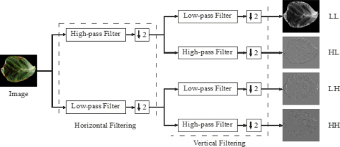
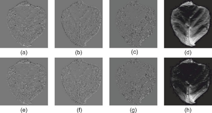
At each stage of the discrete wavelet transform (DWT), image signal will be degraded to two portions with the use of the filters high-pass and low-pass. Averaging operator corresponding to the low-pass filter, sums up the signal’s meaningless statistics. Differential operator, which is also known as the high-pass filter, summarizes the comprehensive signal information. Two distinct one-dimensional transformations result in a two-dimensional conversion [35]. The image is then reduced to two factors by filtering the image along the y-axis and the x-axis, at the end image is divided to sub-bands of four namely high-high (HH), low-high (LH), high-low (HL), and low-low (LL). Figure 2 represents all these four sub-band images for the red spectrum of the Pepper bell Bacterial spot leaf sample. Figure 3 shows the sub-band images for the green and blue spectrum of the same leaf sample.
Haar Wavelet Transform: DWT scales and shifts are commonly based on power of two, rather than generating wavelet coefficients at every conceivable scale, as given in Eq. (1):
$\Psi_{a, b}(i)=2^{-a / 2} \Psi\left(2^{-a}(i-b)\right)$ (1)
where, two denotes the scale base of the image, a denotes the scale parameter and b denotes the shift parameter. A signal s(i) can be expressed in terms of wavelets as given in Eq. (2):
$s(i)=\sum_{a, b} c_{a, b} \Psi_{a, b}(i)$ (2)
where, $\Psi_{a, b}(i)$ denotes the translated mother wavelet. The Haar mother wavelet can be defined as given in Eq. (3):
$\Psi(i)=\left\{\begin{array}{c}1,0 \leq i \leq 1 / 2 \\ -1,1 / 2 \leq i \leq 1 \\ 0, \text { otherwise }\end{array}\right.$ (3)
The function $\Phi(i)$ that used for image decomposition into four sub-band is given in Eq. (4):
$\Phi(i)=\left\{\begin{array}{l}1,0 \leq i \leq 1 \\ 0, \text { otherwise }\end{array}\right.$ (4)
Figure 2. Four sub-bands for red spectrum of Pepper bell Bacterial spot leaf sample
Figure 3. (a-d): Green spectrum, (e-h): Blue spectrum - LL, HL, LH and HH sub-bands, respectively
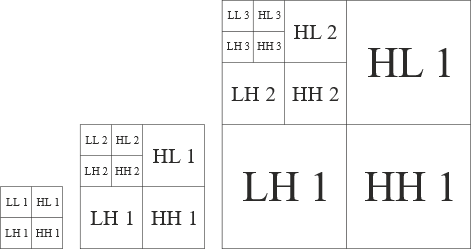
Figure 4 shows multiple levels of sub-bands using Haar wavelet decomposition, where the low-pass filter coefficients LL and LH on the left matrix side and coefficients of high pass filter HL and HH on the right matrix side. Because of the depletion, the entirely modified image has the same size as the original image. The image is then filtered along the y-axis and the x-axis before being reduced by two factors. The red, green, and blue (RGB) spectrum all are processed using the Haar wavelet treatment in order to extract more information about the original image. Thus, in this manner a total of 12 images are generated. However, the LL sub-band gives an approximation image with a low frequency, and as a result, it is disregarded and kept unchanged to retain information for further decomposition of the image. The other sub-bands LH, HL and HH carry more comprehensive information in a different orientation, and are thus used to extract features. The LH, HL and HH sub-bands from the image extracts the features horizontally, vertically and diagonally.
Figure 4. 3-level decomposition of sub-bands using Haar wavelet
4.2 Feature extraction
Feature extraction is the process that is involved in translating the raw data into numerical feature, which can be further processed by retaining the particulars in the master data set. The observed distributed statistical combinations of the intensities at specified points of the image in relative with each other are used for constructing the texture characteristics in statistical analysis. This statistical information is divided further to first, second and higher order depending upon the intensity instances (pixels) in every combination. In this work, two feature extraction techniques are used, namely GLCM, and statistical features. Both of them are discussed below.
4.2.1 GLCM
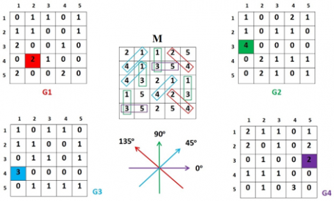
GLCM is a method in which process of extracting second order texture features [36]. Here, the count of rows and columns in the matrix is equal to the count of gray levels (L) in the image. A matrix element E (k, l | ∆p, ∆q) denotes the comparative rate of occurrence accompanied by dual pixels, with intensities k and l, and separated by a pixel distance (∆p, ∆q), occur in a particular neighborhood. Similarly, a matrix element E (k, l | m, θ) denotes the statistical probability values of second-order with respect to the changes that occur between the gray levels k and l, for a distance m at an angle θ. A higher intensity level stores much temporary information, i.e. a L x L matrix for every combination (∆p, ∆q) or (m, θ). An illustration of GLCM formation with five gray levels is shown in Figure 5.
Figure 5. Illustration of GLCM matrix with five gray levels
Here, the original matrix M is used to construct different GLCMs with respect to different angles in each direction [37]. The matrix G1, denoted by red color, represents the frequency for every combination (k, l) for the changes that occur between the gray levels k and l in the original matrix M in the direction at an angle of 135◦ and the distance between pixels is equal to 1. For example, the change between the fourth and second gray levels (4, 2) occurs twice in matrix M at an angle of 135◦ and a distance of 1 pixel. Similarly, the matrix G2, G3 and G4, denoted by green, blue and purple colors, represent the frequency values in the direction at an angle of 90◦, 45◦, and 0◦ respectively.
The GLCMs are particularly sensitive to the size of the texture samples on which they are calculated because of their huge dimension. In result, there is frequent decreased in the count of gray levels.
In this work, five GLCM features, namely Homogeneity, Energy, Dissimilarity, Correlation, and Contrast are utilized for extracting the features from the image. All these are discussed below.
(a) Contrast
Also known as inertia or variance, it denotes the intensity contrast between a pixel and its neighbor over an entire image. The Contrast is given as in Eq. (5):
Contrast $=\sum_{k, l=0}^{L-1}|k-l|^2 E(k, l)$ (5)
where, k and l are the spatial coordinates of the normalized symmetrical GLCM element E (k, l), and L is the gray level.
(b) Correlation
It signifies how a pixel is correlated to its neighbor over an entire image. In other words, it represents the linear dependency of gray levels in neighboring pixels. Its range is [-1, 1], where -1 denotes negatively correlated image, 1 denotes positively correlated image, and NaN for a constant image. The Correlation is given as in Eq. (6):
Correlation $=\sum_{k, l=0}^{L-1} \frac{\left(k-\mu_k\right)\left(l-\mu_l\right) E(k, l)}{\sigma_k \sigma_l}$ (6)
where, µk, µl, σk, σl denote the mean and standard deviation (SD) of pixel intensities, respectively.
(c) Dissimilarity
It denotes the distance between two pixels in the region of interest, and its range is [0, 1]. The Dissimilarity is given as in Eq. (7):
Dissimilarity $=\sum_{k, l=0}^{L-1}|k-l| E(k, l)$ (7)
(d) Energy
Also known as angular second moment or uniformity, it denotes the sum of the squares of the values in GLCM. It is high when the pixels are quite homogeneous or similar. Its range is [0, 1], where 1 is for a constant image. The Energy is given as in Eq. (8):
Energy $=\sum_{k, l=0}^{L-1}(E(k, l))^2$ (8)
(e) Homogeneity
Also known as inverse second moment, it denotes the proximity of spread of pixels in GLCM with respect to the GLCM diagonal. Its range is [0, 1], where 1 is for a diagonal GLCM. The Homogeneity is given as in Eq. (9):
Homogeneity $=\sum_{k, l=0}^{L-1} \frac{E(k, l)}{1+(k-l)^2}$ (9)
4.2.2 Statistical features
In this work, six statistical features are used for extracting the features from the image, namely mean, SD, skewness in the y-axis, skewness in the x-axis, kurtosis in the y-axis, and kurtosis in the x-axis. Each pixel in a colored image is denoted by a vector of three-color spectrum namely blue, green and red, ranging from 0 to 255. The mean for a particular spectrum is the average of all the pixel values in that spectrum. SD is the dispersed value of pixels from the mean in a spectrum. Skewness is a symmetric measure of distribution of pixels in images based on the pixel points on both x and y axis. Thus, pixels in an image can be positively skewed, negatively skewed, or unskewed. Kurtosis signifies whether pixels in image are peaked or flat relative to the normal distribution in both x and y axis. While skewness is the third moment of SD, kurtosis is the fourth moment of SD. The equations for mean, SD, skewness and kurtosis of RGB image with size A x B pixels is given as in from Eq. (10) to (13):
Mean $=\frac{1}{A \cdot B} \sum_{j=1}^{A . B} w_{i, j}$ (10)
$S D=\sqrt{\frac{1}{A \cdot B} \sum_{j=1}^{A . B}\left(w_{i, j}-\bar{w}_l\right)^2}$ (11)
Skewness $=\sqrt[3]{\frac{1}{A . B} \sum_{j=1}^{A . B}\left(w_{i, j}-\bar{w}_l\right)^3}$ (12)
Kurtosis $=\sqrt[4]{\frac{1}{A . B} \sum_{j=1}^{A . B}\left(w_{i, j}-\bar{w}_l\right)^4}$ (13)
where, Wi,j denotes the value of pixel j of ith color spectrum, and $\overline{W l}$ denotes the mean of each spectrum.
4.3 ML classification models
In this work, six ML classification models are used, namely LR, DT, RF, LGBM, AdaBoost, and SVM. All these are discussed below.
4.3.1 Logistic regression
To Unlike the name, LR is used for both binary and multi-class classification in images. In the case of multiple classes, it is also known as Softmax Regression since it uses a softmax classifier for classification [38]. LR estimates the output probability Pi, i=1, ... C, as a C-dimensional vector, giving C estimated probabilities, where C is the count of classes in dataset. The equation for the output probability Pi is given as in Eq. (14):
$p_i=\frac{e^{p_i}}{\sum_{j=0}^C e^{p_j}}$ (14)
The cost function T of the softmax regressor is given as in Eq. (15):
$T=-\left(\sum_{i=1}^N \sum_{j=1}^C 1\left\{p_i=j\right\} \log p_i\right)$ (15)
where, N denotes the input images, and 1 {Pi=j} denotes whether an input image belongs to class j or not.
4.3.2 Decision trees
It is a greedy algorithm with a flowchart like tree structure, which is built in a manner of top-down recursive divide-and conquer. Whereby greedy algorithm is an optimization algorithm that makes the best choice at each step, and it is used for finding the overall, most optimal way to solve a problem. The topmost node is the root, the internal nodes represent a test on the attribute, branch signifies the test outcome and the leaf nodes depict the class labels [39]. Being a greedy algorithm, DT uses information gain approach using Shannon Entropy to minimize the information needed to classify the tuples. The equation for calculating the entropy (Info) is given as in Eq. (16):
Info $=-\sum_{i=1}^C p_i \log _2\left(p_i\right)$ (16)
where, Pi is the probability that a random tuple belongs to class C. After that, the entropy for each feature is calculated, based on which the decision of root attribute is chosen. The equation for attribute entropy (InfoA) is given as in Eq. (17):
$\operatorname{Inf} o_A=\sum_{i=1}^C \sum_{j=1}^v \frac{p_{i j}}{p} \operatorname{Inf} o\left(p_{i j}\right)$ (17)
where, v denotes the distinct samples of particular class i, p denotes the total samples, and Pij denotes the number of samples of type j belonging to class C. The root attribute is decided using the information gain (Ig) of each feature as given in Eq. (18):
$I_g=\operatorname{Info}-\operatorname{Inf} o_A$ (18)
The feature with the highest Ig is used as the root attribute every time. This approach is recursively carried out till there are no features left for further partitioning.
4.3.3 Random forest
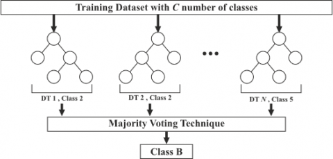
RF is a group classifier used for both classification and regression. It uses a majority voting technique using decisions from several DT, as shown in Figure 6. It overcomes the drawbacks the over-fitting of using a single DT by selecting random training data with replacement to build individual tree [40]. Well defined training data subset will be considered in order to generate DT model for each tree, with the leftover one of three equal parts of training data that which is used for assessing the accuracy of the model. The split criteria for each node in the tree are determined using the second random sample step. The RF model uses certain parameters like input training data, number of trees to build, and the number of predictor variables for creating the binary rule for each split.
Figure 6. Random forest model
4.3.4 LGBM
It is a tree-based gradient boosting technique that optimizes its algorithm by using a random differential loss function. Unlike DT, the choice of splitting the leaf node at each step is done in a more effective manner. While other algorithms grow trees horizontally in a level-by-level manner, LGBM grows trees vertically in a leaf-by-leaf manner. Thus, it develops the leaf with the highest delta loss and has the ability to decrease loss while increasing on the same leaf [41]. This technique can not only handle large scale data with faster training speed but also takes less memory giving better accuracy. Two innovative methods Exclusive Feature Bundling and Gradient based One Side Sampling (GOSS) are used for overcoming constraints of techniques based on histogram in gradient boosting DT.
4.3.5 AdaBoost
It is a sequential ensemble learning method that combines several weak models to form a strong classifier, improving the final predictive performance. For N number of features, the equation of an image i can be given as in Eq. (19):
$F(i)=a_0 f_0(i)+a_1 f_1(i)+\ldots+a_N f_N(i)$ (19)
where, aN denotes the random initial weights, and fN denotes the features [42]. An integral image is created to evaluate the Haar-like features by updating the weights of specific features that maximize the chances of correct classification. Larger weights are assigned to features that offer the classifier a higher number of true positives and true negatives since they are more accurate to the target class. Features that cause a significant amount of false positives and false negatives are given lower weights, with the potential of being assigned a weight of zero.
4.3.6 Support vector machines
Multi-class classification is naturally not supported by SVM. It allows for binary classification by dividing the feature attributes into two groups. Thus, a multi-class problem is broken into several binary classification problems in a recursive manner, also known as one-to-one approach. In a D dimensional space RD, the goal is to design a hyperplane that optimizes the dissociation of the data points to the respective prospective classes. Support vectors are the data points with the shortest distance to the hyperplane (closest points) that are based on the kernel function for efficient class separation [43]. For N training images, it creates two different classes, jϵ{-1, +1}, given as {(i1, j1), ... (iN, jN)} in RD. Images with feature vectors on one part of hyperplane can be labeled as -1, and other part as +1. The equations for separating hyperplane with r number of features is given as in Eq. (20) and (21):
$\sum_{i=1}^r W_i \cdot X_i+b=0$ (20)
$\sum_{i=1}^r W_i \cdot X_i+b=0$ (21)
The main important steps in the field of image classification with numerical features are feature extraction, pre-processing, balancing the dataset and training the ML models. Figure 7 shows the flowchart of the presented work. Here, both the original images (with background) and segmented images (without background) are considered for classification purposes. The modified GLCM technique is approached in this paper to focus only on the leaf portion for extracting the features, as described in (Algorithm 1) and shown in Figure 8(a). For the original images, the GLCM technique and six statistical features are used directly for feature extraction. In the case of segmented images, 2-D discrete Haar wavelet transform is used prior to applying modified GLCM and six statistical features to extract some potential features. Here, the images are divided into four sub-bands, i.e. HH, HL, LH, and LL based on wavelet level 1 decomposition using a symmetric mode. Since the LL image or approximation coefficient is a low-frequency sub-band, it is not considered for extracting the features. Thus, the image is re-scaled to half of its dimension, and the rest three sub-band features are considered for extracting the features. Each channel in an RGB image is represented by 8 bits in a range of 0 to 255. However, after using wavelet transform, the image texture gets affected and the features become out of range. To address this issue, the sub-band images are normalized to the range of 0 to 255, and the values are converted into an 8-bit unsigned integer prior applying the modified GLCM technique. Thus, after normalizing the sub-band images, modified GLCM and statistical features are used on them. In both, the cases of original and segmented images, five GLCM and modified GLCM features and six statistical features are extracted as described in section 4.2 of this paper. The mathematical calculation of all features is described in Table 2. Thirty-three features from original images, ninety-nine features from segmented images, and a total of 132 features are generated through the fusion of features from both types of images.
Figure 7. Flowchart of proposed metho
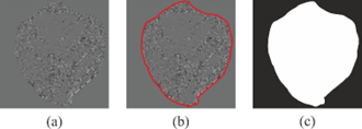
Figure 8. (a) Wavelet image, (b) Image contour, and (c) Masked image
The formal modified GLCM algorithm is represented in Algorithm 1, which computes the co-occurrence matrix accumulation, where the inputs of the algorithm are image i.e. leaf image with dimensions m x n, distance δ has k1 elements, angle θ has k2 elements, levels indicates the level of color gradation in the image typically 256 for an 8-bit image, and mask is an image which highlights the object of input image i.e. leaf part that gives a value of 1 to the pixels of the leaf, and a value 0 to pixels of the leaf background for which the cooccurrence matrix will be counted. The output of algorithm is the co-occurrence matrix accumulation of GLCM. Figure 8(b) illustrates the relevant portion of the leaf for which the co-occurrence matrix should be calculated. whereby the mask of the leaf is generated and passed to Modified GLCM as shown in Figure 8(c). the mask is obtained by using a Sobel filter for edge detection of the leaf. Then experimentally, the threshold operator with a value of 50 is determined to consider the leaf only and eliminate the background.
Table 2. Total features extracted for classification
|
Image Type |
Color Spectrum (a) |
Technique (b) |
Total Features (a) * (b) |
|
|
Original |
Red Green Blue (3) |
GLCM (5) |
15 |
|
|
Statistical Features (6) |
18 |
|||
|
Total |
33 |
|||
|
Image Type |
Color Spectrum (a) |
Wavelet Sub-band (b) |
Technique (c) |
Total Features (a) * (b) * (c) |
|
Segmented |
Red Green Blue (3) |
LH HL HH (3) |
GLCM (5) |
45 |
|
Statistical Features (6) |
54 |
|||
|
Total |
99 |
|||
|
Total Features |
132 |
|||
ALGORITHM 1. MODIFIED GLCM ALGORITHM
|
Input: $[\text { Image }]_{m * n},[\delta]_{k 1},[\theta]_{k 2}$, levels, $[\text { Mask }]_{m * n}$ Output: co- occurences |
|
Algorithm 1 Explanation: Lines 1 and 2 executes the algorithm for all the distance δ and angle θ, respectively. Lines 3 and 4 compute the offset for row and column, given by єr and єc, for each new distance and angle in the loop, respectively. Lines 5 and 6 compute the start and end index of each of the rows (RS, RE) and columns (CS, CE) with considering their offsets. Lines 7 and 8 create loops to compute co-occurrence matrix accumulation after initializing the indexes (RS, RE) for rows and (CS, CE) for columns. Lines 9 and 10 define a condition where pixels in input image corresponding to mask image with a value 0, i.e. background pixels, are ignored. On the contrary, whereas pixels in input image corresponding to mask image with a value 1, i.e. leaf pixels, are passed for the calculation of co-occurrence matrix accumulation. Lines 11 assigns the values of pixel as P. Lines 12 and 13 compute the offset index of current pixel for row r' and column c', where the value of the offset pixel is assigned as P'. Finally, lines 15 and 16 compute the co-occurrence matrix accumulation by adding 1 to its previous value.
However, the features dataset is still imbalanced due to the unequal distribution of classes in the dataset that can affect the classifier’s performance. The count of minority (positive) class tests is very less as compared to the majority (negative) class tests. Most of the forecasts belong to the majority class. The noise persisting in the data comes under the features of the minority class and will be ignored. As a result, the prototype possesses considerable bias. In order to address this issue, the minority class synthetic samples are over-sampled using SMOTE [44]. It is more concerned on the feature space for producing new examples by incorporating with the positive instances which are close. Depending on the over-samplings required, neighbors are picked in random from the k closet required [45]. The synthetic samples are obtained as follows:
1. The variance between the considered feature vector and its closest neighbor is considered.
2. The difference thus obtained will be multiplied with a random value that varies between (0, 1) and then is added to the considered feature vector.
3. In result, an arbitrary location is opted between the two definite characteristics across the line segment.
The balanced data is thus used for classification using the six ML models as discussed in section 4.3 of this paper.
6.1 Dataset description
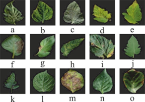
In this paper, the PlantVillage dataset is downloaded from the Kaggle website [46] and used as a dataset for training and testing purposes. It comprises of three different types of crop leaves, namely Pepper bell, Potato, and Tomato. These three crops make 15 various classes of diseased and healthy leaves with a total of 20,638 images, as shown in Table 3. It can be observed that there are two classes of pepper bell, three classes of potato, and ten classes of tomato leaf. The segmented image sample for all the 15 classes of leaf is shown in Figure 9.
Table 3. Composition of PlantVillage dataset
|
SL. No. |
CLASS NAME |
Number of Images |
|
1 |
Tomato mosaic virus |
373 |
|
2 |
Tomato Yellow Leaf Curl Virus |
3208 |
|
3 |
Tomato Target Spot |
1404 |
|
4 |
Tomato Septoria leaf spot |
1771 |
|
5 |
Tomato Early blight |
1000 |
|
6 |
Tomato Leaf Mold |
952 |
|
7 |
Tomato Spider mites Two spotted spider mite |
1676 |
|
8 |
Tomato Late blight |
1909 |
|
9 |
Tomato Bacterial spot |
2127 |
|
10 |
Tomato healthy |
1591 |
|
11 |
Pepper bell Bacterial spot |
997 |
|
12 |
Pepper bell healthy |
1478 |
|
13 |
Potato Late blight |
1000 |
|
14 |
Potato healthy |
152 |
|
15 |
Potato Early blight |
1000 |
|
|
Total |
20,638 |
Figure 9. (a) Tomato Spider mites Two spotted spider mite, (b) Tomato Yellow Leaf Curl Virus, (c) Tomato Target Spot, (d) Tomato Septoria leaf spot, (e) Tomato Bacterial spot, (f) Potato Late blight, (g) Tomato Late blight, (h) Tomato Leaf Mold, (i) Tomato Early blight, (j) Tomato healthy, (k) Tomato mosaic virus, (l) Potato healthy, (m) Potato Early blight, (n) Pepper bell healthy, and (o) Pepper bell Bacterial spot
6.2 Experimental setup and parameters
Every experiment enclosed in this paper is performed in a Windows 10 system version 21H1, with 64-bit operating system and 8 GB RAM. Python 3.8.10 was used as the programming language and all the experiments were performed on Spyder platform. RunwayML is used as a platform to eliminate the background from the images using U2Net architecture. The various experimental factors that are considered in the analysis are represented in the Table 4.
Table 4. Experimental parameters
|
Technique |
Parameter |
Value |
|
GLCM |
distance |
3 |
|
direction |
0o (East GLCM) |
|
|
Dataset Split |
Training |
80% |
|
Testing |
20% |
|
|
AdaBoost |
classifier |
RandomForestClassifier |
|
max_depth |
7 |
|
|
n_estimators |
15 |
|
|
DT |
random_state |
42 |
|
RF |
n_estimators |
15 |
|
random_state |
42 |
|
|
criterion |
Entropy |
|
|
LR |
random_state |
42 |
|
penalty |
L2 |
|
|
SVM |
decision_function_shape |
ovo |
|
kernel |
rbf |
|
|
LGBM |
learning_rate |
0.05 |
|
Objective |
multiclass |
|
|
max_depth |
10 |
7.1 Classification results
The results obtained after applying all the parameters described in Table 4 and using the six ML techniques on the balanced dataset are presented in Table 5. It shows accuracy values obtained using different combinations of features in original as well as segmented dataset. The highest accuracy values obtained in each set of combination is marked in red bold, while the second highest accuracy is marked in green bold. Table 5 shows the highest accurate value of 94.76% is obtained using the LGBM classifier when all the features are combined using both original and segmented datasets, i.e. Both (c) and (f) columns. Similarly, the second highest accuracy value of 93.51% is obtained using the SVM classifier for the same combination. The second-best combination is acquired when GLCM is used with original dataset features, i.e. Both (c) and (d) columns. The lowest accuracy is obtained when only statistical features are used with the segmented dataset, i.e., column (e). Further, it can be observed that the LGBM classifier performs best in most of the cases, followed by the SVM classifier. However, the DT classifier performs the poorest among all the classifiers used in every combination. Another experimentation comparing the accuracy and mean absolute error (MAE) of imbalanced v/s balanced dataset, and wavelet level 1 (L1) v/s level 2 (L2) decomposition is presented in Table 6. The MAE denotes the difference of average between the actual and measured value over total number of data samples as in Eq. (22):
$M A E=\frac{1}{n} \sum_{i=1}^n\left|y_l^{\prime}-y_i\right|$ (22)
where, yi is true value, $y_i^{\prime}$ is prediction value, and n is the total number of data points. From the Table 6, it can be observed that there is a significant difference is noticed in accuracy and MAE values between the imbalanced and balanced datasets.
Table 5. Accuracy values obtained using different combination of features and ML models
|
ML MODELS |
DT |
AdaBoost |
LR |
RF |
SVM |
LGBM |
|
|
Both (c) & (f) |
80.65 |
89.43 |
91.07 |
91.84 |
93.51 |
94.76 |
|
|
Both (c) & (e) |
77.02 |
86.57 |
88.13 |
88.67 |
91.39 |
93.18 |
|
|
Both (c) & (d) |
78.98 |
87.36 |
89.80 |
90.45 |
92 |
93.69 |
|
|
Both (b) & (f) |
74.58 |
83.05 |
85.21 |
86 |
88.87 |
88.76 |
|
|
Both (a) & (f) |
75.36 |
84.19 |
86.54 |
86.11 |
89.25 |
90.82 |
|
|
Both (b) & (e) |
71.13 |
80.57 |
82.96 |
82.49 |
85.09 |
85.68 |
|
|
Both (a) & (d) |
71.98 |
81.45 |
84.01 |
84.33 |
86.62 |
87.14 |
|
|
Without Background |
Both (f) |
67.49 |
76.62 |
78 |
78.20 |
79.23 |
79.80 |
|
SF (e) |
53.44 |
61.36 |
62.79 |
62.24 |
64.91 |
66.27 |
|
|
GLCM (d) |
60.03 |
69.21 |
69.95 |
70.10 |
71.22 |
72 |
|
|
With Background |
Both (c) |
75.40 |
84 |
86.92 |
87.05 |
90.28 |
92.11 |
|
SF (b) |
65.35 |
75.03 |
76.38 |
75.97 |
77.85 |
77.24 |
|
|
GLCM (a) |
69.57 |
78.60 |
80.87 |
81.14 |
83.44 |
82.92 |
|
Table 6. Comparison between unbalanced and balanced dataset
|
ML MODELS |
DT |
AdaBoost |
LR |
RF |
SVM |
LGBM |
ML MODELS |
|
Balanced Dataset Wavelet (L2) |
MAE |
0.882 |
0.495 |
0.407 |
0.441 |
0.315 |
0.229 |
|
Accuracy |
78.94 |
88.15 |
90.33 |
89.90 |
92.37 |
94.02 |
|
|
Balanced Dataset Wavelet (L1) |
MAE |
0.791 |
0.417 |
0.358 |
0.332 |
0.246 |
0.205 |
|
Accuracy |
80.65 |
89.43 |
91.07 |
91.84 |
93.51 |
94.76 |
|
|
Imbalanced Dataset |
MAE |
1.664 |
1.216 |
0.845 |
0.707 |
0.672 |
0.566 |
|
Accuracy |
64.58 |
76.26 |
80.12 |
83.01 |
83.81 |
85.63 |
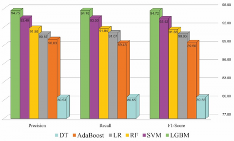
Figure 10. Precision, Recall and F1-score for ML models used (x100)
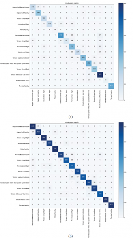
Figure 11. Confusion matrix (a) Imbalanced dataset, (b) Balanced dataset
The SMOTE balanced dataset provides quite better accuracy than the imbalanced dataset. In case of wavelet, L1 decomposition gives better accuracy and less MAE values than L2 decomposition. However, there is not a significant difference between both the levels. Figure 10 shows the plots for precision, recall, and F1-score values obtained for all the ML models. The ratio of the precisely forecasted positive samples and the absolute anticipated positive samples is termed as Precision. The ratio of the precisely predicted positive samples and all positive samples in actual class is termed as Recall. The harmonic weighted average balance persisted between precision and recall is the F1-score. Where the equations for Precision, Recall, and F1-score are denoted in Eq. (23)-(25) respectively:
Precision $=\frac{\text { True Positive }}{\text { True Positive }+\text { False Positive }}$ (23)
Recall $=\frac{\text { True Positive }}{\text { True Positive }+\text { False Negative }}$ (24)
F1 $=2 * \frac{\text { Precision } * \text { Recall }}{\text { Precision }+\text { Recall }}$ (25)
A confusion matrix is a 2x2 matrix which visualizes and summarizes a classifier performance based on a group of test data whose real values are known prior. Each column of the matrix represents the instances in a predicted class while each row represents the instances in an actual class (or vice versa). The diagonal of the matrix represents the number of correct classifications for the same class and the rest represents the number of misclassifications between two classes. The confusion matrix obtained in the case of both imbalanced and balanced datasets is shown in Figure 11. From Figure 11(a) denoting the confusing matrix for the imbalanced dataset, it can be observed that the misclassified samples in the minority classes are more than half of its test set due to the model training the majority classes better than the minority ones. This dataset is not good enough for distinguishing because of the similarity between some samples which leads to misclassified samples. However, this issue is addressed using SMOTE, as shown in Figure 11(b).
7.2 Discussion
From Table 5, it can be generalized that the DT classifier is not a good choice for image datasets. Images are purely based on local connections between the features, i.e., the proximity of the pixel to its neighbors. Because DT does not account for this, the outcomes are subpar and greatly influenced by noise. They also do not perform well with large datasets. Further, with large number of features, DT needs overfitting of data because they can split on many distinct combinations of features, that leads to high variance and error in output with high inaccuracy. AdaBoost classifier, on the other hand, generalizes well with large data and is less susceptible to overfitting. However, it considers only important features in the dataset, ignoring the rest. Thus, not considering all the pixel features in images can lead to not getting good results at times. Though there is not a significant difference between LR and RF, the RF classifier however performs well than LR in most cases. Image features are hierarchical and complicated, and deducing them using LR with a single linear layer is sometimes difficult. RF using an ensemble learning technique eliminates the overfitting problem in DT. However, using a large number of trees is sometimes ineffective for real-time predictions. Coming to SVM, this classifier has the ability to model complicated non-linear boundaries, especially in high dimensional spaces. The Gaussian RBF kernel works quite well with non-linear image data, making it less prone to overfitting. For this reason, it is one of the best ML models used in image classification. Finally, the LGBM classifier, being a powerful histogram-based gradient boosted algorithm, performs the best among all other classifiers. It is much compatible even with large complex datasets, and has a faster training speed among all other classifiers because of its high speed. Instaead of level-wise split approach, leaf-wise split strategy is used for building remarkable complicated trees, which acts as a major element to obtain greater accuracy.
From Table 5, two more points can also be generalized. First, GLCM features, either taken alone or combined provide better accuracy than statistical features. This is because GLCM features are based on second-order statistics, while the statistical features used in this work are based on first order statistics. The first-order statistics provide features that offer information about the image’s gray-level distribution. However, the statistics will not provide details regarding the comparative placements of numerous gray levels of images. These characteristics will not be able to conclude if all gray levels of low value can be grouped together or can be swapped for further gray levels of higher value [47]. However, this data may be obtained from the GLCM technique, which evaluates second-order image statistics and considers pixels in pairs. Second, combination of GLCM and modified GLCM and statistical features provides better accuracy, than either of these used alone. All of these features work together to produce a high level of discrimination between two types of images.
Similarly, from Table 6, two points can be generalized. First, the accuracy of an imbalanced dataset is less than that of a balanced dataset, because of the significant bias obtained due to the presence of less number of bulk predictions and minority class samples for the majority class samples. Thus, SMOTE is used for addressing this issue which in turn provides quite a good accuracy. Second, the accuracy of wavelet L1 is better than that of L2 decomposition. Decomposing an image leads to a decrease in Bits per Pixel (BPP), Peak Signal-to-Noise ratio (PSNR), compression ratio [48], and an increase in root mean squared error (RMSE), mean squared error (MSE) and MAE. This in turn leads to a loss of information. Thus, wavelet L1 preserves more information than wavelet L2, and thus provides better accuracy.
Plant disease detection is one of the crucial challenges in the agricultural industry. Diagnosing illnesses in plants at an early stage is critical for avoiding severe losses in annual crop production. Both ML and DL take part crucial contribution in the detection and classification of plant diseases. This paper concentrates on the classification of plant diseases using six ML classifiers. GLCM, modified GLCM and statistical features were used for extracting the potential features of the plant images. Different combinations of features using original as well as the segmented dataset are used, and it was observed that the LGBM and SVM models perform the best among all other classifiers. As the analysis is performed using the dataset with a limited number of samples, further work can be carried out to analyse samples by considerably increasing the dataset. Moreover, some robust deep neural networks such as Hybrid CNN, Generative Adversarial Network, etc. can also be used to extract potential features from the images for a better classification of the diseases. Thus, future works would rely on using the complete dataset along with some powerful feature extraction techniques and DL models for the detection and classification of plant diseases.
|
Notation |
Description |
|
θ |
The angle between two different gray levels |
|
δ |
The distance between two different gray levels |
|
єr |
Row offset |
|
єc |
Column offset |
|
RS, RE |
Start and end index of rows respectively |
|
CS, CE |
Start and end index of columns respectively |
|
P |
Pixel value of current index |
|
r' |
Offset index of current pixel for row |
|
c' |
Offset index of current pixel for column |
|
P' |
Pixel value of offset index |
[1] Beghin, T., Cope, J.S., Remagnino, P., Barman, S. (2010). Shape and texture based plant leaf classification. In International conference on advanced concepts for intelligent vision systems, pp. 345-353. https://doi.org/10.1007/978-3-642-17691-3_32
[2] Chaki, J., Parekh, R. (2012). Plant leaf recognition using Gabor filter. International Journal of Computer Applications, 56(10). https://doi.org/10.5120/8927-3000
[3] Vibhute, A., Bodhe, S.K. (2012). Applications of image processing in agriculture: A survey. International Journal of Advanced Networking and Applications, 52(2): 34-40. https://doi.org/10.5120/8176-1495
[4] Pradhan, A.K., Swain, S., Kumar Rout, J. (2022). Role of machine learning and cloud-driven platform in IoT-based smart farming. In Machine Learning and Internet of Things for Societal Issues, pp. 43-54. https://doi.org/10.1007/978-981-16-5090-1_4
[5] Barbedo, J.G.A. (2018). Impact of dataset size and variety on the effectiveness of deep learning and transfer learning for plant disease classification. Computers and Electronics in Agriculture, 153: 46–53. https://doi.org/10.1016/j.compag.2018.08.013
[6] Usharani, B. (2022). House plant leaf disease detection and classification using machine learning. In Mundada, M. et al (eds) Deep Learning Applications for Cyber-Physical Systems, IGI Global, pp. 17–26. https://doi.org/10.4018/978-1-7998-8161-2.ch002
[7] Sabrol, H., Satish, K. (2016). Tomato plant disease classification in digital images using classification tree. In 2016 International Conference on Communication and Signal Processing (ICCSP), pp. 1242-1246. https://doi.org/10.1109/ICCSP.2016.7754351
[8] Shruthi, U., Nagaveni, V., Raghavendra, B.K. (2019). A review on machine learning classification techniques for plant disease detection. In 2019 5th International Conference on Advanced Computing & Communication Systems (ICACCS), pp. 281-284. https://doi.org/10.1109/ICACCS.2019.8728415
[9] Yang, X., Guo, T. (2017). Machine learning in plant disease research. March, 31: 1. https://doi.org/10.18088/ejbmr.3.1.2017.pp6-9
[10] Panchal, P., Raman, V.C., Mantri, S. (2019). Plant diseases detection and classification using machine learning models. In 2019 4th International Conference on Computational Systems and Information Technology for Sustainable Solution (CSITSS), pp. 1-6. https://doi.org/10.1109/CSITSS47250.2019.9031029
[11] Akhtar, A., Khanum, A., Khan, S.A., Shaukat, A. (2013). Automated plant disease analysis (APDA): performance comparison of machine learning techniques. In 2013 11th International Conference on Frontiers of Information Technology, pp. 60-65. https://doi.org/10.1109/FIT.2013.19
[12] Arasakumaran, U., Johnson, S.D., Sara, D. and Kothandaraman, R. (2022). An enhanced identification and classification algorithm for plant leaf diseases based on Deep Learning. Traitement du Signal, 39(3). https://doi.org/10.18280/ts.390328
[13] Bayram, H.Y., Bingol, H. and Alatas, B. (2022). Hybrid deep model for automated detection of tomato leaf diseases. Traitem12ent du Signal, 39(5): 1781-1787. https://doi.org/10.18280/ts.390537
[14] Wagle, S.A. (2021). A deep learning-based approach in classification and validation of tomato leaf disease. Traitement du Signal, 38(3). https://doi.org/10.18280/ts.380317
[15] Bauer, S.D., Korc, F., Förstner, W., Van Henten, E.J., Goense, D., Lokhorst, C. (2009). Investigation into the classification of diseases of sugar beet leaves using multispectral images. Precision Agriculture, 9: 229-238.
[16] Liu, L., Zhang, W., Shu, S., Jin, X. (2013). Image recognition of wheat disease based on RBF support vector machine. In 2013 International Conference on Advanced Computer Science and Electronics Information (ICACSEI 2013), pp. 307-310. https://doi.org/10.2991/icacsei.2013.77
[17] Panigrahi, K.P., Das, H., Sahoo, A.K., Moharana, S.C. (2020). Maize leaf disease detection and classification using machine learning algorithms. In Progress in Computing, Analytics and Networking, pp. 659-669. https://doi.org/10.1007/978-981-15-2414-1_66
[18] Tian, J., Hu, Q., Ma, X., Han, M. (2012). An improved KPCA/GA-SVM classification model for plant leaf disease recognition. Journal of Computational Information Systems, 8(18): 7737-7745.
[19] Ramesh, S., Hebbar, R., Niveditha, M., Pooja, R., Shashank, N., Vinod, P.V. (2018). Plant disease detection using machine learning. In 2018 International conference on design innovations for 3Cs compute communicate control (ICDI3C), pp. 41-45. https://doi.org/10.1109/ICDI3C.2018.00017
[20] Shrivastava, V.K., Pradhan, M.K. (2021). Rice plant disease classification using color features: a machine learning paradigm. Journal of Plant Pathology, 103(1): 17-26. https://doi.org/10.1007/s42161-020- 00683-3
[21] Elhariri, E., El-Bendary, N., Hassanien, A.E. (2014). Plant classification system based on leaf features. In 2014 9th International Conference on Computer Engineering & Systems (ICCES), pp. 271-276. https://doi.org/10.1109/ICCES.2014.7030971
[22] Lee, S.H., Chan, C.S., Mayo, S.J., Remagnino, P. (2017). How deep learning extracts and learns leaf features for plant classification. Pattern Recognition, 71: 1-13. https://doi.org/10.1016/j.patcog.2017.05.015
[23] Tan, J., Chang, S.W., Abdul-Kareem, S., Yap, H.J., Yong, K.T. (2018). Deep learning for plant species classification using leaf vein morphometric. IEEE/ACM Transactions on Computational Biology and Bioinformatics, 17(1): 82-90. https://doi.org/10.1109/TCBB.2018.2848653
[24] Sembiring, A., Away, Y., Arnia, F., Muharar, R. (2021). Development of concise convolutional neural network for tomato plant disease classification based on leaf images. In Journal of Physics: Conference Series, 1845(1): 012009. https://doi.org/10.1088/1742-6596/1845/1/012009
[25] Turkoglu, M., Yanikoğlu, B., Hanbay, D. (2022). PlantDiseaseNet: Convolutional neural network ensemble for plant disease and pest detection. Signal, Image and Video Processing, 16(2): 301-309. https://doi.org/10.1007/s11760-021-01909-2
[26] Khamparia, A., Saini, G., Gupta, D., Khanna, A., Tiwari, S., de Albuquerque, V.H.C. (2020). Seasonal crops disease prediction and classification using deep convolutional encoder network. Circuits, Systems, and Signal Processing, 39(2): 818-836. https://doi.org/10.1007/s00034-019-01041-0
[27] Hassan, S.M., Maji, A.K. (2022). Plant disease identification using a novel convolutional neural network. IEEE Access, 10: 5390–5401. https://doi.org/10.1109/ACCESS.2022.3141371
[28] Mittal, A., Gupta, H. (2022). An experimental evaluation in plant disease identification based on activation-reconstruction generative adversarial network. In 2nd International Conference on Advance Computing and Innovative Technologies in Engineering (ICACITE), pp. 361–366. https://doi.org/10.1109/ICACITE53722.2022.9823924
[29] Pahurkar, A., Deshmukh, R. (2022). PDMBM: Design of a high-efficiency plant disease classification method using multiparametric bio inspired modelling. In International Conference on Sustainable Computing and Data Communication Systems (ICSCDS), pp. 1607–1615. https://doi.org/10.1109/ICSCDS53736.2022.9761034
[30] Kong, J., Wang, H., Yang, C., Jin, X., Zuo, M., Zhang, X. (2022). A spatial feature-enhanced attention neural network with high-order pooling representation for application in pest and disease recognition. Agriculture, 12(4): 500. https://doi.org/10.3390/agriculture12040500
[31] Aurangzeb, K., Akmal, F., Khan, M.A., Sharif, M., Javed, M.Y. (2020). Advanced machine learning algorithm based system for crops leaf diseases recognition. In 2020 6th Conference on Data Science and Machine Learning Applications (CDMA), pp. 146-151. https://doi.org/10.1109/CDMA47397.2020.00031
[32] Tan, L., Lu, J., Jiang, H. (2021). Tomato leaf diseases classification based on leaf images: A comparison between classical machine learning and deep learning methods. AgriEngineering, 3(3): 542-558. https://doi.org/10.3390/agriengineering3030035
[33] Xian, T.S., Ngadiran, R. (2021). Plant diseases classification using machine learning. In Journal of Physics: Conference Series, 1962(1): 012024. https://doi.org/10.1088/1742-6596/1962/1/012024
[34] Rahman, A., Al Foisal, M., Rahman, M., Miah, M., Mridha, M.F. (2022). Deep-CNN for plant disease diagnosis using low resolution leaf images. In Machine Learning and Autonomous Systems, pp. 459-469. https://doi.org/10.1007/978-981-16-7996-4_33
[35] Kiaee, N., Hashemizadeh, E., Zarrinpanjeh, N. (2019). Using GLCM features in Haar wavelet transformed space for moving object classification. IET Intelligent Transport Systems, 13(7): 1148-1153. https://doi.org/10.1049/iet-its.2018.51924
[36] Mohanaiah, P., Sathyanarayana, P., GuruKumar, L. (2013). Image texture feature extraction using GLCM approach. International Journal of Scientific and Research Publications, 3(5): 1-5.
[37] Vyas, R., Kanumuri, T., Sheoran, G., Dubey, P. (2017). Co-occurrence features and neural network classification approach for iris recognition. In 2017 Fourth International Conference on Image Information Processing (ICIIP), pp. 1-6. https://doi.org/10.1109/ICIIP.2017.8313730
[38] Dong, Q., Zhu, X., Gong, S. (2019). Single-label multi-class image classification by deep logistic regression. In Proceedings of the AAAI conference on artificial intelligence, 33(1): 3486-3493. https://doi.org/10.1609/aaai.v33i01.33013486
[39] Agarwal, C., Sharma, A. (2011). Image understanding using decision tree based machine learning. In Proceedings of the 5th international Conference on Information Technology & Multimedia, pp. 1-8. https://doi.org/10.1109/ICIMU.2011.6122757
[40] Tabbakh, A., Rout, J.K., Rout, M. (2021). Analysis and prediction of the survival of titanic passengers using machine learning. In Advances in Distributed Computing and Machine Learning, pp. 297-304. https://doi.org/10.1007/978-981-15-4218-3_29
[41] Pradhan, A.K., Swain, S., Rout, J.K., Ray, N.K. (2022). Prediction of stroke disease using different types of gradient boosting classifiers. In Advances in Data Computing, Communication and Security, pp. 337-346. https://doi.org/10.1007/978- 981-16-8403-6_30
[42] Asil, H., Bagherzadeh, J. (2020). A new approach to image classification based on a deep multiclass AdaBoosting ensemble. International Journal of Electrical and Computer Engineering, IAES Institute of Advanced Engineering and Science, 10(5): 4872-4880. https://doi.org/10.11591/ijece.v10i5.pp4872-4880
[43] Thai, L.H., Hai, T.S., Thuy, N.T. (2012). Image classification using support vector machine and artificial neural network. International Journal of Information Technology and Computer Science, 4(5): 32-38. https://doi.org/10.5815/ijitcs.2012.05.0
[44] Tabbakh, A. (2021). Bankruptcy prediction using robust machine learning model. Turkish Journal of Computer and Mathematics Education (TURCOMAT), 12(10): 3060-3073. https://doi.org/10.17762/TURCOMAT.V12I10.4957
[45] Chawla, N.V., Bowyer, K.W., Hall, L.O., Kegelmeyer, W.P. (2002). SMOTE: synthetic minority over-sampling technique. Journal of Artificial Intelligence Research, 16: 321-357. https://doi.org/10.1613/jair.953
[46] Kaggle. (2018). The dataset is taken from the Kaggle opensource link. https://www.kaggle.com/datasets/emmarex/plantdisease, Last accessed May 2022.
[47] Hlaing, K.N.N. (2015). First order statistics and GLCM based feature extraction for recognition of Myanmar paper currency. In Proceedings of the 31st IIER International Conference, Bangkok, Thailand, pp. 1-6.
[48] Vigneswara, T. (2016). Effects of decomposition levels of wavelets in image compression algorithms. Journal of Biomedical Sciences, 5(4): 0-0. https://doi.org/10.4172/2254-609X.100043