Mehmet Zahit Uzun* | Yuksel Celik | Erdal Basaran
© 2022 IIETA. This article is published by IIETA and is licensed under the CC BY 4.0 license (http://creativecommons.org/licenses/by/4.0/).
OPEN ACCESS
This study proposes a framework for defining ME expressions, in which preprocessing, feature extraction with deep learning, feature selection with an optimization algorithm, and classification methods are used. CASME-II, SMIC-HS, and SAMM, which are among the most used ME datasets in the literature, were combined to overcome the under-sampling problem caused by the datasets. In the preprocessing stage, onset, and apex frames in each video clip in datasets were detected, and optical flow images were obtained from the frames using the FarneBack method. The features of these obtained images were extracted by applying AlexNet, VGG16, MobilenetV2, EfficientNet, Squeezenet from CNN models. Then, combining the image features obtained from all CNN models. And then, the ones which are the most distinctive features were selected with the Particle Swarm Optimization (PSO) algorithm. The new feature set obtained was divided into classes positive, negative, and surprise using SVM. As a result, its success has been demonstrated with an accuracy rate of 0.8784 obtained in our proposed ME framework.
CNN, FarneBack, micro expression, optical flow, PSO, SVM
Recognizing human emotions from facial expressions can be misleading and deceptive; emotions can be hidden by applying other facial expressions, but MEs are used to understand real emotions [1] because MEs occurring unconsciously. ME occurs at high risk when people try to control and suppress facial expressions. It cannot be controlled and occurs with low intensity (thin) and short duration (fast) [2-4]. These expressions containing real emotions [5] are facial expressions that occur between 1/25 and 1/2 second and occur in a few small areas of the face, unlike full expressions [6].
The formation processes of micro-expressions consist of 3 parts: start, apex, and offset [7]. Apex formation is known as the peak of a ME. Considering the difficulties of developing methods that can cope with short-term and low intensity [8], this study focuses on the apex framework, where the expressions are most intense.
The remainder of the article is organized as follows: The following section details some previous related work. Brief information about the publicly available dataset used is given in section 3. The existing model, feature selection method, data augmentation method, machine learning method, optimization method, and the proposed method are briefly presented in section 4. Experimental results are given in section 5. The discussion is presented in section 6. Finally, section 7 includes conclusion statements and future work.
The models in the ME studies consist of three parts: preprocessing, feature extraction, and classification. The preprocessing phase consists of separating the non-face area and detecting, aligning, and cropping the face region to prevent the effect of head movement [9]. In studies on face detect, DRMF method [10, 11] Active Shape Model (ASM) 68-point method [4, 8, 12] were used. Dlib machine learning toolkit of the OpenCV library used for both detection and alignment are used [9, 13, 14].
Methods used as Feature Extraction are divided into traditional methods and data-oriented methods; these conventional models are Optical Flow, LBP, and its derivatives. Optical flow is a technique that detects motion variation between two video frames [9, 15-17]. Local binary patterns (LBP) are used to extract texture features from gray images [4]. The derivative of LBP, which encodes both spatial and temporal information, is used LBP-TOP [5, 8, 18, 19].
Deep learning methods are another method used in ME called data-oriented methods. In addition, using deep learning architecture from raw images, both feature extraction and classification can be done [20, 21]. Transfer learning methods have been used to overcome the problem when data is scarce [10, 20, 22]. Another method used in classification is SVM and its derivatives which are of great importance for machine learning [2, 3, 5, 8].
Based on the scarcity of datasets in ME studies and the idea that CNN-based studies in this area are limited [23], a hybrid model with traditional and data-oriented is proposed as our motivation in the study. In addition, CASME-II, SAMM, SMIC datasets, which are the most widely used and publicly available spontaneous micro-expressions, were used in our study.
Publicly available Spontaneous ME datasets are CASME, CAME-II, (CAME)^2, SAMM, and SMIC datasets. CASME-II is a higher version of CAME. The SMIC, SAMM, and CASMEII datasets are currently used composite or separate in many studies [9, 12, 23, 24] as they are the most comprehensive [8], widely used [12, 25], state-of-the-art [6], spontaneous ME datasets, and available to the public.
In addition to the limited number of available data sets and sampling [8], which is one of the difficulties related to ME, the unbalanced sample distribution in emotion classes also creates another problem (CASME-II fear 2, sadness 4, others 99, happiness 32). Therefore, many studies were used composite data sets that combined the spontaneous ME datasets [22-25]. In these studies, the 3 most used datasets regarding spontaneous ME's are Casme-II [26], SAMM [27], and SMIC [28]. CASME-II has 7 emotion classes. These are disgust, fear, happiness, other, repression, sadness, and surprise. SAMM has 8 classes. These are anger, contempt, disgust, fear, happiness, others, sadness, and surprise. SMIC-HS has 3 classes. These are negative, positive, and surprise. In order to use the 3 datasets together, CASME-II and SAMM datasets with the highest number of classes are matched to the class number of the SMIC dataset, which has the lowest number of classes. The "other" class is not used in this pairing to avoid confusion. This study was combined the most commonly used 3 datasets and created a composite dataset with 3 classes [29]. These classes are negative (Repression, anger, contempt, disgust, fear, and sadness) 266, positive (happiness) 112, and surprise (surprise) 88. Table 1 shows the features of these data sets.
In the studies conducted with ME, two types of frames were selected sequence-based (video) and apex-based [23]. This study focuses on the most density expression frame, using the apex-based used in recent studies. Only two frames are considered in the apex-based design. These are onset frame and apex frame.
Data in other classes were increased after optical flow processing by taking the negative class with the largest sample of data as a reference. At the end of the data increase, each class equals 266 optical flow image data. Data in classes with low samples are increased by rotating 90°, 180°, 270° degrees.
Table 1. Properties of the spontaneous dataset used
|
Datasets |
Casme-II |
SMIC-HS |
SAMM |
|
Subjects |
24 |
16 |
28 |
|
Samples |
152 |
191 |
121 |
|
Negative |
92 |
92 |
80 |
|
Positive |
32 |
54 |
26 |
|
Surprise |
28 |
45 |
15 |
|
Frame Rates |
200 fps |
100 fps |
200 fps |
|
Resolution |
640*480 |
640*480 |
2040*1088 |
|
Face Resolutions |
280*340 |
190*230 |
400*400 |
The architecture of the proposed model consists of four steps: preprocessing, feature extraction, feature selection, and classification. The structure of the model is given in Figure 1.
Normalized ME images were obtained from apex frame spot, face detection, face landmark, face alignment, and face crop operations in the preprocessing step. In the second step, ME motion properties were obtained by applying the FarneBack optical flow method to the images. Then these images were reproduced by using the rotation augmentation method. By applying CNN models to the augmented dataset, feature maps of the images were obtained from the fully connected layer of each model. 5,000 features were obtained by combining 1,000 features obtained from each of five different CNN models. With the PSO algorithm, the best features of the images for ME recognition were filtered, the feature selection step was realized. Finally, ME classification was performed using different kernels of the SVM algorithm in the classification stage. A detailed explanation of the methods we use in our proposed ME recognition classification framework and information on their use are below:
Figure 1. ME classification framework architecture
4.1 Preprocessing
In the proposed study, Apex single frame images were taken from ME dataset frames. The Apex frame was chosen because it has the highest ME density in a video frame sequence [30]. While the index of this frame is provided in Casme-II and SAMM datasets, it is not provided in the SMIC dataset, so the D&C-RoIs (Divide and Conquer-Region of Interest) [31] technique, which automatically finds its approximation position, has been developed. Because the D&C-RoIs technique provides successful performance in apex detection, it has been used in ME studies [6, 25, 32]. The D&C-RoI method includes the feature descriptor LBP and divide&conquer techniques. LBP calculates the features of the face regions of each frame in a video sequence. Then, the feature difference of each frame is calculated by taking the onset frame as a reference. The divide & conquer algorithm determines the position (index) of the apex frame which has the maximum difference.
The Apex frame was obtained by calculating the RoI regions in each frame and calculating the correlation between the first frame and other frames with the LBP descriptor [31]. The calculation of the correlations of the first frame and the remaining frames using LBP is given in Eq. (1) [25].
$d=\frac{\sum_{i=1}^B h_{1 i} x h_{2 i}}{\sqrt{\sum_{i=1}^B h_{1 i}^2 x \sum_{i=1}^B h_{2 i}^2}}$ (1)
here, h1 is the first frame, h2 is the other frames, and B is the number of boxes in the h1 and h2 histograms. The difference ratio of LBP features (1-d) between the eyebrow, eye, and mouth, the three most effective ROIs in ME recognition, is compared. The ROI with the highest difference ratio is selected. Finally, a divide-and-conquer strategy is applied [25, 31] to seek frames that have maximum facial muscle changes. According to the divide and conquer strategy, a video clip frame sequence is divided into subsequences. The correlation coefficients of the frames are summed in each sub-array. The index with the largest sum is kept, and the rest is discarded. It continues until the frame with the maximum value is found [2].
In Figure 2, the positions of the frames in a video sequence in the micro-expression and their optical flow data of these positions are seen. This example is the happiness sample found in the Casme-II dataset.
Figure 2. Onset, apex and offset in ME video sequence
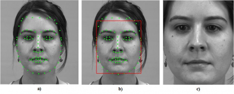
Since CASME-II and SMIC samples have preprocessed formats, they were not required preprocessing. However, since SAMM samples did not go through any preprocessing step, preprocessing was performed on the SAMM dataset before extracting the optical flow properties of the images. Face detection, alignment, cropping, and recording processes were applied to the samples in the SAMM dataset, respectively. Functions in OpenCV and dlib libraries are used. Since the micro-expression recognition task focuses on certain parts of the face, regions outside the facial areas (hair, neck, background, ear, etc.) in the video frame may cause performance loss in expression recognition. A preprocessing task is performed to dispose of these noises’ areas. Thus, the irrelevant data for micro-expression recognition are excluded from the process. After detecting the face regions with the detector function in the dlib library, the trained model in the same library, which predicts the face region with 81 points, is used. The outer points are positioned to frame the outer part of the front view of the face, and the inner points are positioned as the mouth, eyes, eyebrows, and nose. The facial area was cropping and recorded after aligning the points on the temples of the forehead at the top and slightly above the chin at the bottom. After cropping face regions, all images' dimensions were resized to 224 x 224 for VGG16, MobileNetV2, EfficientNetB0, and 227x227 for AlexNet, and SqueezeNet.
In Figure 3, Face Detection, Face Mark, Face Alignment and Face Cropping operations are shown on an example of the SAMM dataset.
Figure 3. a) Face detection, face mark, b) Face alignment c) Face cropping operations
4.2 Optical flow
Optical flow is a method that can capture subtle movements between two frames and small changes in pixels according to the assumption of constant brightness [21, 33]. This method is used in areas such as action recognition, action detection, object tracking. Density-based Farneback [34] is used to detect the optical flow of each point. This method, which is also used in micro-expression studies [9, 35] was used in this study because of its many advantages. In addition to the advantage of fast computation, the Farneback optical flow technique, which has a pyramidal decomposition approach and produces relatively fewer errors in analyzing facial movements, is preferred [36]. Farneback optical flow estimates the approximate neighborhoods of each pixel using polynomial expansion with a quadratic polynomial. Mathematical equations of Farneback optical flow are given in Eqns. (2)-(6) [34].
$f_1(x)=x^T A_1 x+B_1^T x+c_1$ (2)
here, A is a symmetric matrix, b is a vector, and c1 is a scalar. A new f2 signal is generated using a global shift d.
$f_2(x)=f_1(x-d)$
$=(x-d)^T A_1(x-d)+b_1^T(x-d)+c_1$
$=x^T A_1 x+\left(b_1-2 A d\right)^T x+d^T A_1 d-b_1^T d+c_1$
$=x^T A_2 x+b_2^T x+c_2$ (3)
In Eq. (4), if the coefficients in quadratic polynomials are equalized, Eqns. (5) and (6) are obtained.
$A_1=A_2$ (4)
$b_2=b_1-2 A_1 d$ (5)
$d=-\frac{1}{2} A_1^{-1}\left(b_2-b_1\right)$ (6)
Figure 4. Optic flow processes with the onset and apex frame
In Figure 4, it is shown that the motion between the initial (onset) frame where the motion starts and the apex frame, where the expression is maximum, is obtained by optical flow.
The figure shown is an example of EP01_01f in Subject 19's in the CASME-II dataset, labeled happiness.
4.3 Data augmentation
Table 1 shows that negative emotions have more samples in all three data sets when compared to positive and surprise emotions. Class imbalance in the datasets makes classification in favor of the class with the large sample size of the SVM classifier [37]. The data augmentation technique was used due to the sampling imbalance in the micro-expression datasets used in this study. Thus, by creating a dataset that has balanced sampling, results in which the SVM to be used can classify more accurately are aimed. The classes in our dataset are 266 for negative sample, 112 for positive sample, and 88 for surprise sample. Data in other classes were increased by taking the negative class with the largest sample of data as a reference. At the end of the data increase, each class equals 266 optical flow image data. Data in classes with low samples are increased by rotating 90°, 180°, 270° degrees.
4.4 Convolutional neural network
1,000 deep features are obtained from fully connected layers of 5 different CNN models. These are the FC8 layer from VGG16, FC8 layer from AlexNet, Pool10 layer from SqueezeNet, Logits layer from MobileNetV2, and dense|MatMul layer from EfficientNetB0. 1,000 features taken from each layer are brought to the same plane using the MinMaxScalar method. This data is then combined and fed into the input of the PSO algorithm with combined 5,000 features. In Table 2, the models and the layers of the models from which the features are obtained are given.
Table 2. Selected layers of CNNs
|
CNN model |
Features extraction layer |
|
VGG16 |
FC 8 |
|
AlexNet |
FC 8 |
|
SqueezeNet |
Pool10 |
|
MobileNetV2 |
Logits |
|
EfficientNetB0 |
dense|MatMul |
4.5 Particle swarm optimization
In this study, the PSO optimization algorithm was used for feature selection. The parameters used in the experiment were respectively randomly adjusted in the range of Population Dimension (D) 1000, which gives the number of extracted features, Population Size (N) 10, which gives the number of populations, and Population Matrix (X) $0>x_i^t>1$. In cases where $x_i^t>0.5$, feature selection is made, otherwise feature selection is not made. When the Iteration of number 100 is taken, the number of function evaluations is N*100=1000, and the Number of KNN (k) is 5. PSO parameters are taken as 2 for Cognitive factor, 2 for Social factor, and 0.9 for Inertia weight. The fitness calculation equation is given in Eq. (7).
EroorRate $=1-$ ACC
SF (SelectedFeatures $)=\sum_{i=0}^D x_i=1$
Fitnes Function $=$ alpha $*$ ErrorRate $+$ beta*(S F / D) (7)
here, SF represents the total selected features, while the accuracy rate obtained in the K-NN classification of ACC selected features is taken as alpha=0.99, beta=0.01.
A total of 5,000 deep features obtained from 5 different CNNs are given to the selected optimization algorithm to choose the best features. According to the algorithm results, 2,746 different deep features of deep features were selected and provided as input data to the SVM classification.
4.6 Support vector machine
SVM has been used in research because it is found to be successful in statistical learning, modeling of data optimization, object detection as well as micro-expression recognition tasks [3, 5, 8]. In this study, linear, quadratic, finegaussian, and cubic kernel functions were used with SVM, and its superiority in the micro-expression recognition task was compared. The mathematical equations of the cores used in our study are given in Eqns. (8)-(11) [38].
Linear $\operatorname{SVM} k\left(x_i, x_j\right)=x_i^T x_j+c, c$ is a constant (8)
Gaussian $k\left(x_i, x_j\right)=\exp \left(-\frac{\left\|x_i-x_j\right\|^2}{2 S^2}\right)$ (9)
Cubic $k\left(x_i, x_j\right)=\left(x_i^T x_j+1\right)^3$ (10)
Quadratic $k\left(x_i, x_j\right)=1-\frac{\left\|x_i-x_j\right\|^2}{\left\|x_i-x_j\right\|^2+c}$ (11)
here, Xi and Xj are input vectors, k () is kernel function. S is the bandwidth parameter, which determines how quickly the similarity metric drops as the samples move away from each other.
4.7 Performance metrics
In machine learning, other measures besides accuracy are used to evaluate the success of the model on the data set and to analyze the data in more detail [39-41]. The accuracy value alone gives only how many of the predictions made are correct. Therefore, in this study, the confusion matrix is used to analyze the classification performance of the models used. The parameters used in the complexity matrix are True Positive (TP), False Positive (FP), False Negative (FN), and True Negative (TN). The mathematical equations of these measurements are given in Eqns. (12)-(17) [42].
$\operatorname{Accuracy}($ Acc $)=\frac{T P+T N}{T P+F P+T N+F N}$ (12)
Sensitivity $(S n)=\frac{T P}{T P+F N}$ (13)
$\operatorname{Specificity}(S p)=\frac{T N}{F P+T N}$ (14)
Recall $=\frac{T P}{T P+F N}$ (15)
Precision $=\frac{T P}{T P+F P}$ (16)
$F_{\text {score }}=\frac{2 * \text { Precision } * \text { Recall }}{\text { Precision }+\text { Recall }}$ (17)
In addition, model performance was evaluated with a ten-fold cross-validation method. In the cross-validation method, the data set is divided into ten equal parts that nine parts are training data rest one part is test data. This situation continues until each part has been test-data once.
Experimental test results were obtained using deep learning, classification, and optimization algorithms on micro-expression data sets.
First, the classification performances of VGG16, SqueezeNet, MobileNetV2, EfficientNet, AlexNet models of the new integrated and augmented data sets formed by combining the three selected data sets are given in Table 3.
The hyperparameters of the first and second experimental studies using CNN models are the same. The Maximum Epoch Value at which the whole dataset is trained is set to 32, the Mini Batch Size trained in each iteration is set to 16, the Initial Learning Rate value is 0.001, the Validation Frequency value is 50, Learn Rate Drop Factor value is 0.1, and the Learn Rate Drop Period value is 16 has been set. In the integrated data set in Table 3, Vgg16 and AlexNet had the highest accuracy rates of 0.7143, while Vgg16 showed the highest performance with a value of 0.6626 in sensitivity measurement. In precision and F1 measurements, AlexNet showed the best performance with 0.7011 and 0.6739, respectively, while vgg16 was superior in specificity and precision measurement. In the results obtained using the same hyperparameters in the augmented data set, the Vgg16 model increased its performance compared to its values in the integrated data set while outperforming other models. The VGG16 model in the augmented data set achieved accuracy 0.8083, sensitivity 0.8083, specificity 0.9042, precision 0.8269, and f1 score of 0.8114, giving it superiority over other models in the micro-expression recognition task.
In the second experimental study, 1000 deep features are obtained from fully connected layers of 5 different CNN models. These are the FC8 layer from VGG16, FC8 layer from AlexNet, Pool10 layer from SqueezeNet, Logits layer from MobileNetV2, and dense|MatMul layer from EfficientNetB0.
Next, the combined feature vectors were classified with linear, quadratic, finegaussian, cubic kernels of SVM. Thus, the performance of SVM kernels and CNN classifiers was compared, then the advantages of SVM kernels in the micro expression recognition task were compared. In classification measurements made with the quadratic core, Squeezenet is superior to other models with 0.7866 accuracies, 0.7860 sensitivity, 0.8932 specificity, 0.8011 precision, and 0.7858 F1 value. In classification with SVM using linear core, EfficientNet were achieved better results than others in all performance measurements. Accuracy value of 0.6653, sensitivity value of 0.6652, specificity value of 0.8325, precision value of 0.6697 and F1 value of 0.6663 were obtained. With the classification of the data set using the Finegaussian kernel, Squeezenet has the highest accuracy rate of 0.6485, and it is the model with the highest value. While it was superior to other models in sensitivity, specificity and F1 values, it was the most successful model with vgg16 0.8235 in precision. The Cubic was the core that gave the highest accuracy, sensitivity, specificity, and F1 values in classifying 1000 feature maps. Accuracy 0.8033 ratio, sensitivity 0.8027 ratio, specificity 0.9016 ratio and F1 0.8012 ratio were obtained. Detailed information about all results is shown in Table 4.
In the third experimental study, when the combined 5,000 features were classified with the SVM classifier and compared with the previous values we obtained, the results were observed to improve further. In Table 5, the precision value obtained with the finegaussian kernel was the most successful with 0.8506, while the cubic kernel gave better results in all other values. In the classification made with the Cubic core, the accuracy ratio was 0.8117, the sensitivity ratio was 0.8120, the specificity ratio was 0.906, and the f1 ratio was 0.8114.
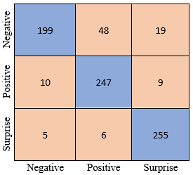
In the fourth experimental study, 2,760 distinctive features were selected using PSO analysis on the 5000-feature data set obtained by combining these features. When the SVM classifier is used with these selected distinctive features, an improvement has been observed in the performance of other measurements except the precision measurement. Table 6 shows the performance of each kernel after feature selection. Accordingly, from the quadratic kernel that gave the best results, the accuracy value was 0.8243, the sensitivity value was 0.8245, the specificity value was 0.9121, the precision value was 0.8275, and the F1 value was 0.8232. The confusion matrix of the Quadratic kernel is given in Figure 5.
Figure 5. Complexity matrix of our model without cross-validation
Figure 6. Complexity matrix of our model with cross-validation
In our fifth and last experimental study, the data set was divided into 10 parts using the cross-validation method, 1 part was set as test data, and the remaining 9 part was set as training data (k=10). This operation allows all parts to be used cyclically as training and test data. Thus, each sample on the data set acts as both a test set and a training set. This situation provides a more efficient result [39]. In Table 7, the classification performances of SVM kernels with the cross-validation process of 2760 data obtained after strong feature selection are listed. Accordingly, the cubic core has the most successful performance and the highest performance values in the experiments. Accordingly, cubic was the core with the most successful performance, and the highest performance values were obtained in the experiments. The results obtained are accuracy 0.8784, sensitivity 0.8784, specificity 0.9392, precision 0.8765, respectively. The confusion matrix of the cubic core is given in Figure 6.
Table 3. CNN results with performance metrics
|
Model |
Dataset |
Acc (%) |
Sen (%) |
Spe (%) |
Pre (%) |
F1 (%) |
|
VGG16 |
Composed |
0.7143 |
0.6626 |
0.8260 |
0.6820 |
0.6656 |
|
Squeezenet |
0,6857 |
0,62 |
0,8027 |
0,6627 |
0,6370 |
|
|
MobilenetV2 |
0.6143 |
0.4437 |
0.7221 |
0.6159 |
0.4491 |
|
|
EfficientNet |
0.6000 |
0.4613 |
0.7391 |
0.5138 |
0.4686 |
|
|
AlexNet |
0.7143 |
0.6600 |
0.8150 |
0.7011 |
0.6739 |
|
|
VGG16 |
Augmented |
0.8083 |
0.8083 |
0.9042 |
0.8269 |
0.8114 |
|
Squeezenet |
0.7125 |
0.7125 |
0.8562 |
0.7180 |
0.7137 |
|
|
MobilenetV2 |
0.5583 |
0.5583 |
0.7792 |
0.5568 |
0.5507 |
|
|
EfficientNet |
0.6083 |
0.6083 |
0.8042 |
0.6142 |
0.6082 |
|
|
AlexNet |
0.7667 |
0.7667 |
0.8833 |
0.7695 |
0.7651 |
Table 4. Classification results of 1,000 CNN feature maps used with SVM kernels
|
Model |
Kernel |
Acc (%) |
Sen (%) |
Spe (%) |
Pre (%) |
F1 (%) |
|
VGG16 |
Quatric |
0.6653 |
0.6659 |
0.8325 |
0.6619 |
0.6633 |
|
Squeezenet |
0.7866 |
0.7860 |
0.8932 |
0.8011 |
0.7858 |
|
|
MobilenetV2 |
0.6904 |
0.6906 |
0.8452 |
0.6894 |
0.6876 |
|
|
EfficientNet |
0.7782 |
0.7784 |
0.8890 |
0.7806 |
0.7769 |
|
|
AlexNet |
0.6987 |
0.6989 |
0.8493 |
0.6988 |
0.6988 |
|
|
VGG16 |
Lineer |
0.5565 |
0.5570 |
0.7781 |
0.5599 |
0.5568 |
|
Squeezenet |
0.6234 |
0.6230 |
0.8116 |
0.6443 |
0.6256 |
|
|
MobilenetV2 |
0.5858 |
0.5861 |
0.7929 |
0.5840 |
0.5841 |
|
|
EfficientNet |
0.6653 |
0.6652 |
0.8325 |
0.6697 |
0.6663 |
|
|
AlexNet |
0.5816 |
0.5820 |
0.7907 |
0.5816 |
0.5817 |
|
|
VGG16 |
Finegaussian |
0.6234 |
0.6224 |
0.8113 |
0.8235 |
0.6146 |
|
Squeezenet |
0.6485 |
0.6499 |
0.8250 |
0.8058 |
0.6463 |
|
|
MobilenetV2 |
0.4268 |
0.4292 |
0.7146 |
0.7886 |
0.3360 |
|
|
EfficientNet |
0.6360 |
0.6348 |
0.8176 |
0.8263 |
0.6257 |
|
|
AlexNet |
0.5816 |
0.5806 |
0.7904 |
0.8045 |
0.5674 |
|
|
VGG16 |
Cubic |
0.7143 |
0.7146 |
0.8571 |
0.7108 |
0.7118 |
|
Squeezenet |
0.8033 |
0.8027 |
0.9016 |
0.8151 |
0.8012 |
|
|
MobilenetV2 |
0.7448 |
0.7449 |
0.8724 |
0.7434 |
0.7430 |
|
|
EfficientNet |
0.7741 |
0.7742 |
0.8869 |
0.7796 |
0.7732 |
|
|
AlexNet |
0.7322 |
0.7324 |
0.8662 |
0.7405 |
0.7327 |
Table 5. Classification results of CNN feature concatenating with SVM kernels
|
Kernel |
Acc (%) |
Sen (%) |
Spe (%) |
Pre (%) |
F1 (%) |
|
Quatric |
0.7908 |
0.7911 |
0.8955 |
0.7946 |
0.7897 |
|
Linear |
0.7029 |
0.7029 |
0.8516 |
0.7101 |
0.7053 |
|
Fine gaussian |
0.7280 |
0.7278 |
0.8637 |
0.8506 |
0.7306 |
|
Cubic |
0.8117 |
0.8120 |
0.9060 |
0.8159 |
0.8114 |
Table 6. Classification results with SVM kernels after PSO analysis
|
Kernel |
Acc (%) |
Sen (%) |
Spe (%) |
Pre (%) |
F1 (%) |
|
Quatric |
0.8243 |
0.8245 |
0.9121 |
0.8275 |
0.8232 |
|
Linear |
0.7322 |
0.7324 |
0.8660 |
0.7445 |
0.7321 |
|
Fine gaussian |
0.6820 |
0.6813 |
0.8407 |
0.8376 |
0.6833 |
|
Cubic |
0.8159 |
0.8162 |
0.9079 |
0.8202 |
0.8140 |
Table 7. Classification results with SVM kernels after PSO analysis and cross-validation
|
Kernel |
Acc (%) |
Sen (%) |
Spe (%) |
Pre (%) |
F1 (%) |
|
Quatric |
0.8484 |
0.8484 |
0.9242 |
0.8508 |
0.8469 |
|
Linear |
0.7306 |
0.7306 |
0.8653 |
0.7323 |
0.7299 |
|
Fine gaussian |
0.6729 |
0.6729 |
0.8365 |
0.7526 |
0.6712 |
|
Cubic |
0.8784 |
0.8784 |
0.9392 |
0.8839 |
0.8765 |
Table 8. Our best performance without cross-validation and with cross-validation
|
Kernel |
Acc (%) |
Sen (%) |
Spe (%) |
Pre (%) |
F1 (%) |
|
Quadratic without cross-validation |
0.8243 |
0.8245 |
0.9121 |
0.8275 |
0.8232 |
|
Cubic with cross-validation |
0.8784 |
0.8784 |
0.9392 |
0.8839 |
0.8765 |
Table 9. Comparison of recent successful models
|
Methods |
Accuracy |
F1 Score |
Dataset |
|
OFF-ApexNet [6] |
0.746 |
0.710 |
SMIC+CASME-II +SAMM |
|
From macro to Micro [20] |
0.747 |
0.64 |
CASME-II +SAMM |
|
Residual Network with Micro-Attention [22] |
0.763 |
0.668 |
CASME-II +SAMM |
|
STSTNet [25] |
0.769 |
0.739 |
SMIC+CASME-II +SAMM |
|
STSTNet+GA [23] |
0.859 |
0.837 |
SMIC+CASME-II +SAMM |
|
CNN+PSO+SVM (Proposed) |
0.8784 |
0.8765 |
SMIC+CASME-II +SAMM |
Nowadays, classification of ME images has an important place in many fields such as forensic informatics, security, and education. In our study, it was observed that the F1 scores of accuracy rates could not exceed 72% in the classification made using CNN models on the combined data set. To increase the success, it has been observed that the success rates increase in the classification made by duplicating the data set with the data augmentation technique. When the increasing rates are examined, While the accuracy rate exceeding 80% and the F1 measurement rate exceeding 81% were obtained. Table 3 that values up to 90% were obtained in other measurements. From this, it can be concluded that the data augmentation technique will positively affect many CNN models in increasing the ME recognition performance. In the classification using four different SVM kernels in Table 4, made with feature maps taken from the last connected layers of CNN models, the experimental results could not exceed the performance when Table 3 was taken as the basis. The results obtained by combining the feature maps in Table 5, on the other hand, partially step up onto the performance. It can be concluded that there is a need for more besides different classification techniques. It can be concluded that the reason for this is that more than different classification techniques are needed. As a matter of fact, in the next step, the results obtained from quadratic and cubic kernels with the experiment using the PSO algorithm for the selection of the best features caused a noticeable increase in Table 6. In the accuracy and F1 measurements, which reached the highest values, the values of 0.8243 and 0.8232 were obtained, respectively. In this study, the highest performance measurements were obtained among the experiments carried out so far. Thus, it has been observed that the data obtained by feature selection has a positive effect on increasing the ME recognition performance. In addition, Table 7 shows that the experiment using the PSO algorithm and cross-validation technique with SVM kernels there were significant improvements in classification performance for all measurement values compared to the initial values. More concretely, compared to the best measurement values in the composite data set in Table 3, the performance increase was 16.41% for accuracy, 21.58% for sensitivity, 11.32% for specificity, 18.28% for precision, and 20.26% for F1. Confusion matrices and AUC-ROC graphs of methods and techniques are given to analyze ME classification performance in depth. The best results obtained in our experiments are shown in Table 8.
In addition, a comparison of our work with the latest technology models in the ME field is presented in Table 9. The results show that our model is competitive and satisfactory.
In the study [15], the success of different optical flow methods in ME recognition is presented in Table 3. Recognition results produced using the Farneback method are given as the two best methods that outperform each other in different block sizes, together with TVL1. In addition, it has been shown as another advantage for the Faneback method, which is faster than the others in calculating the analysis of facial movements [36]. It should be considered that modified Pso derivatives and different SVM kernels can give more positive results in increasing ME recognition accuracy.
This study presents a new framework for ME recognition tasks consisting of traditional and data-driven methods. The framework consists of these steps are; preprocessing, feature extraction, feature selection, and classification, respectively. These multiple steps are applied to image frames containing facial expressions. With the preprocessing step, the images are normalized. Then, optical flow and CNN techniques were applied in the feature extraction stage, and PSO analysis was applied in the feature selection stage. Finally, after classifying the selected feature data with SVM, the results were compared with other studies using SVM for classification. The most important advantage of the FarneBack optical flow method is its low time cost and its success in analyzing facial movements. One of the essential originalities of our work is quadratic, fine gaussian, and cubic SVM core functions that we used in micro-expression recognition classification. Another important originality of our work is PSO feature selection in micro-expression recognition. The advantages of these kernel functions in the micro-expression recognition task were compared in different experiments. In this study, it has been shown that artificially increasing the data set obtained by an optical flow can improve classification accuracy. Depending on this data augmentation method, it has been observed that it can improve the model's performance by 9% to 13%. Feature selection and cross-validation processes with the PSO algorithm contributed positively to the performance of our model. For the future in micro-expression recognition, the task showed promising results. As a result, it has been shown that 16% to 20% better results are obtained compared to the experimental test results obtained with the proposed framework. Our framework achieved the highest classification accuracy, achieving 87.84% accuracy and 87.65% F1 values on the three combined datasets. In addition, the specificity value reached 0.9392, the sensitivity 0.8784, and the precision 0.8839. We will continue to design models with higher real-time ME recognition accuracy and model performance in the future.
[1] Patel, D., Hong, X., Zhao, G. (2016). Selective deep features for micro-expression recognition. In 2016 23rd international conference on pattern recognition (ICPR), Cancun, Mexico, pp. 2258-2263. https://doi.org/10.1109/ICPR.2016.7899972
[2] Liong, S.T., See, J., Wong, K., Phan, R.C.W. (2018). Less is more: Micro-expression recognition from video using apex frame. Signal Processing: Image Communication, 62: 82-92. https://doi.org/10.1016/j.image.2017.11.006
[3] Liu, Y.J., Zhang, J.K., Yan, W.J., Wang, S.J., Zhao, G., Fu, X. (2015). A main directional mean optical flow feature for spontaneous micro-expression recognition. IEEE Transactions on Affective Computing, 7(4): 299-310. https://doi.org/10.1109/TAFFC.2015.2485205
[4] Huang, X., Wang, S. J., Zhao, G., Piteikainen, M. (2015). Facial micro-expression recognition using spatiotemporal local binary pattern with integral projection. In Proceedings of the IEEE International Conference on Computer Vision Workshops, pp. 1-9. https://doi.org/10.1109/ICCVW.2015.10
[5] Wang, S.J., Yan, W.J., Li, X., Zhao, G., Zhou, C.G., Fu, X., Yang, M.H., Tao, J. (2015). Micro-expression recognition using color spaces. IEEE Transactions on Image Processing, 24(12): 6034-6047. https://doi.org/10.1109/TIP.2015.2496314
[6] Gan, Y.S., Liong, S.T., Yau, W.C., Huang, Y.C., Tan, L.K. (2019). OFF-ApexNet on micro-expression recognition system. Signal Processing: Image Communication, 74: 129-139. https://doi.org/10.1016/j.image.2019.02.005
[7] Xia, Z., Feng, X., Peng, J., Peng, X., Zhao, G. (2016). Spontaneous micro-expression spotting via geometric deformation modeling. Computer Vision and Image Understanding, 147: 87-94. https://doi.org/10.1016/j.cviu.2015.12.006
[8] Li, X., Hong, X., Moilanen, A., Huang, X., Pfister, T., Zhao, G., Pietikäinen, M. (2017). Towards reading hidden emotions: A comparative study of spontaneous micro-expression spotting and recognition methods. IEEE Transactions on Affective Computing, 9(4): 563-577. https://doi.org/10.1109/TAFFC.2017.2667642
[9] Zhao, S., Tao, H., Zhang, Y., Xu, T., Zhang, K., Hao, Z., Chen, E. (2021). A two-stage 3D CNN based learning method for spontaneous micro-expression recognition. Neurocomputing, 448: 276-289. https://doi.org/10.1016/j.neucom.2021.03.058
[10] Wang, S.J., Li, B.J., Liu, Y.J., Yan, W.J., Ou, X., Huang, X., Xu, F., Fu, X. (2018). Micro-expression recognition with small sample size by transferring long-term convolutional neural network. Neurocomputing, 312: 251-262. https://doi.org/10.1016/j.neucom.2018.05.107
[11] Yao, L., Xiao, X., Cao, R., Chen, F., Chen, T. (2020). Three stream 3D CNN with SE block for micro-expression recognition. In 2020 International Conference on Computer Engineering and Application (ICCEA), Guangzhou, China, pp. 439-443. https://doi.org/10.1109/ICCEA50009.2020.00101
[12] Xia, Z., Hong, X., Gao, X., Feng, X., Zhao, G. (2019). Spatiotemporal recurrent convolutional networks for recognizing spontaneous micro-expressions. IEEE Transactions on Multimedia, 22(3): 626-640. https://doi.org/10.1109/TMM.2019.2931351
[13] Li, X., Yu, J., Zhan, S. (2016). Spontaneous facial micro-expression detection based on deep learning. In 2016 IEEE 13th International Conference on Signal Processing (ICSP), pp. 1130-1134. https://doi.org/10.1109/ICSP.2016.7878004
[14] Takalkar, M.A., Xu, M. (2017). Image based facial micro-expression recognition using deep learning on small datasets. In 2017 International Conference on Digital Image Computing: Techniques and Applications (DICTA), pp. 1-7. https://doi.org/10.1109/DICTA.2017.8227443
[15] Liong, S.T., Gan, Y.S., Zheng, D., Li, S.M., Xu, H.X., Zhang, H.Z., Lyu, R.K., Liu, K.H. (2020). Evaluation of the spatio-temporal features and GAN for micro-expression recognition system. Journal of Signal Processing Systems, 92(7): 705-725. https://doi.org/10.1007/s11265-020-01523-4
[16] Zhou, L., Mao, Q., Xue, L. (2019). Dual-inception network for cross-database micro-expression recognition. In 2019 14th IEEE International Conference on Automatic Face & Gesture Recognition (FG 2019), pp. 1-5. https://doi.org/10.1109/FG.2019.8756579
[17] Ben, X., Jia, X., Yan, R., Zhang, X., Meng, W. (2018). Learning effective binary descriptors for micro-expression recognition transferred by macro-information. Pattern Recognition Letters, 107: 50-58. https://doi.org/10.1016/j.patrec.2017.07.010
[18] Duan, X., Dai, Q., Wang, X., Wang, Y., Hua, Z. (2016). Recognizing spontaneous micro-expression from eye region. Neurocomputing, 217: 27-36. https://doi.org/10.1016/j.neucom.2016.03.090
[19] Wang, Y., See, J., Phan, R.C.W., Oh, Y.H. (2015). Efficient spatio-temporal local binary patterns for spontaneous facial micro-expression recognition. PloS One, 10(5): e0124674. https://doi.org/10.1371/journal.pone.0124674
[20] Peng, M., Wu, Z., Zhang, Z., Chen, T. (2018). From macro to micro expression recognition: Deep learning on small datasets using transfer learning. In 2018 13th IEEE International Conference on Automatic Face & Gesture Recognition (FG 2018), pp. 657-661. https://doi.org/10.1109/FG.2018.00103
[21] Liu, N., Liu, X., Zhang, Z., Xu, X., Chen, T. (2020). Offset or onset frame: A multi-stream convolutional neural network with CapsuleNet module for micro-expression recognition. In 2020 5th International Conference on Intelligent Informatics and Biomedical Sciences (ICIIBMS), pp. 236-240. https://doi.org/10.1109/ICIIBMS50712.2020.9336412
[22] Wang, C., Peng, M., Bi, T., Chen, T. (2020). Micro-attention for micro-expression recognition. Neurocomputing, 410: 354-362. https://doi.org/10.1016/j.neucom.2020.06.005
[23] Liu, K.H., Jin, Q.S., Xu, H.C., Gan, Y.S., Liong, S.T. (2021). Micro-expression recognition using advanced genetic algorithm. Signal Processing: Image Communication, 93: 116153. https://doi.org/10.1016/j.image.2021.116153
[24] Liu, Y., Du, H., Zheng, L., Gedeon, T. (2019). A neural micro-expression recognizer. In 2019 14th IEEE International Conference on Automatic Face & Gesture Recognition (FG 2019), pp. 1-4. https://doi.org/10.1109/FG.2019.8756583
[25] Liong, S.T., Gan, Y.S., See, J., Khor, H.Q., Huang, Y.C. (2019). Shallow triple stream three-dimensional CNN (STSTNet) for micro-expression recognition. In 2019 14th IEEE International Conference on Automatic Face & Gesture Recognition (FG 2019), pp. 1-5. https://doi.org/10.1109/FG.2019.8756567
[26] Yan, W.J., Li, X., Wang, S.J., Zhao, G., Liu, Y.J., Chen, Y.H., Fu, X. (2014). CASME II: An improved spontaneous micro-expression database and the baseline evaluation. PloS One, 9(1): e86041. https://doi.org/10.1371/journal.pone.0086041
[27] Davison, A. K., Lansley, C., Costen, N., Tan, K., Yap, M. H. (2016). Samm: A spontaneous micro-facial movement dataset. IEEE Transactions on Affective Computing, 9(1): 116-129. https://doi.org/10.1109/TAFFC.2016.2573832
[28] Li, X., Pfister, T., Huang, X., Zhao, G., Pietikäinen, M. (2013). A spontaneous micro-expression database: Inducement, collection and baseline. In 2013 10th IEEE International Conference and Workshops on Automatic Face and Gesture Recognition (FG), pp. 1-6. https://doi.org/10.1109/FG.2013.6553717
[29] See, J., Yap, M. H., Li, J., Hong, X., Wang, S.J. (2019). MEGC 2019–the second facial micro-expressions grand challenge. In 2019 14th IEEE International Conference on Automatic Face & Gesture Recognition (FG 2019), pp. 1-5. https://doi.org/10.1109/FG.2019.8756611
[30] Li, Y., Huang, X., Zhao, G. (2018). Can micro-expression be recognized based on single apex frame? In 2018 25th IEEE International Conference on Image Processing (ICIP), pp. 3094-3098. https://doi.org/10.1109/ICIP.2018.8451376
[31] Liong, S.T., See, J., Wong, K., Le Ngo, A.C., Oh, Y.H., Phan, R. (2015). Automatic apex frame spotting in micro-expression database. In 2015 3rd IAPR Asian Conference on Pattern Recognition (ACPR), pp. 665-669. https://doi.org/10.1109/ACPR.2015.7486586
[32] Gan, Y.S., Liong, S.T. (2018). Bi-directional vectors from apex in CNN for micro-expression recognition. In 2018 IEEE 3rd International Conference on Image, Vision and Computing (ICIVC), pp. 168-172. https://doi.org/10.1109/ICIVC.2018.8492829
[33] Huang, W. (2021). Elderly depression recognition based on facial micro-expression extraction. Traitement du Signal, 38(4): 1123-1130. https://doi.org/10.18280/ts.380423
[34] Farnebäck, G. (2003). Two-frame motion estimation based on polynomial expansion. In Scandinavian Conference on Image Analysis, pp. 363-370. https://doi.org/10.1007/3-540-45103-X_50
[35] Allaert, B., Bilasco, I.M., Djeraba, C. (2018). Advanced local motion patterns for macro and micro facial expression recognition. arXiv preprint arXiv:1805.01951.
[36] Allaert, B., Ward, I.R., Bilasco, I.M., Djeraba, C., Bennamoun, M. (2019). Optical flow techniques for facial expression analysis: Performance evaluation and improvements. ArXiv, abs/1904.11592.
[37] Li, Y., Huang, X., Zhao, G. (2020). Joint local and global information learning with single apex frame detection for micro-expression recognition. IEEE Transactions on Image Processing, 30: 249-263. https://doi.org/10.1109/TIP.2020.3035042
[38] Bassma, G., Tayeb, S. (2018). Support vector machines for improving vehicle localization in urban canyons. In MATEC Web of Conferences, 200: 00004.
[39] Tonkal, Ö., Polat, H., Başaran, E., Cömert, Z., Kocaoğlu, R. (2021). Machine learning approach equipped with neighbourhood component analysis for DDoS attack detection in software-defined networking. Electronics, 10(11): 1227. https://doi.org/10.3390/electronics10111227
[40] Merghani, W., Davison, A.K., Yap, M.H. (2018). A review on facial micro-expressions analysis: Datasets, features and metrics. arXiv preprint arXiv:1805.02397.
[41] Basaran, E., Cömert, Z., Çelik, Y., Budak, Ü., Sengür, A. (2020). Otitis media diagnosis model for tympanic membrane images processed in two-stage processing blocks. IOP Sci, 14: 1-27.
[42] Başaran, E., Cömert, Z., Çelik, Y. (2020). Convolutional neural network approach for automatic tympanic membrane detection and classification. Biomedical Signal Processing and Control, 56: 101734. https://doi.org/10.1016/j.bspc.2019.101734