Pandu Wicaksono* | Samuel Philip | Islam Nur Alam | Sani M. Isa
© 2022 IIETA. This article is published by IIETA and is licensed under the CC BY 4.0 license (http://creativecommons.org/licenses/by/4.0/).
OPEN ACCESS
Data in the health sector are often lacking and unbalanced. It is because collecting data takes time and many resources. One example is sleep apnea data which takes about 8–10 hours to get data and uses specialized hardware like polysomnography (PSG). This study proposes a data augmentation technique to handle unbalanced data using DCGAN and several deep learning models such as 1D-CNN, ANN, LSTM, and 1D-CNN+LSTM as a classifier for apnea detection. The DCGAN architecture used is CNN on the generator and discriminator. DCGAN will create new synthetic data by mimicking the original dataset. This experiment uses a dataset from PhysioNet, the Apnea-ECG, and the MIT-BIH PSG Database. Furthermore, the dataset is preprocessed to remove noise, and the features are extracted manually. The test scenario is to create 10% synthetic data and 50% sleep apnea data to be added to the original dataset. Then compare the performance of multiple deep learning models before and after adding data. The results indicate that augmentation with DCGAN can improve the performance of almost all models, with the highest increase of 1.78% on the 1D-CNN+LSTM model and 4.80% on the LSTM model for the Apnea-ECG and MIT-BIH datasets, respectively.
DCGAN, deep learning, ECG, imbalance data, sleep apnea
Sleep apnea is a disorder that interferes with breathing while sleeping. This disorder can cause sufferers to often wake up from sleep because of difficulty breathing. There are three types of sleep apnea, namely, Obstructive Sleep Apnea (OSA), Central Sleep Apnea (CSA), and Mixed Sleep Apnea (MSA). With OSA being the most common sleep disorder. In most cases, this disorder often affects people of old age and people who are overweight (obese). This disorder can be diagnosed using polysomnography (PSG), the gold standard in the world of health. Getting this data takes a long time [1] and costs between $3000-$6000 for every test [2].
With the rapid development of artificial intelligence (AI), AI can be used in various fields of life, including the health sector. Implementing AI in the health sector, especially in detecting sleep apnea, can promise a cheap and fast solution to dealing with various problems. Some examples of research conducted in detecting sleep apnea are supervised machine learning and deep learning methods. Mukherjee et al. [3] used the deep learning ensemble model technique, which produces the highest accuracy of 85.58%. Then Banluesombatkul et al. [4] tried to create a filter at the preprocessing stage. Filtering is used to remove disturbing noise and the accuracy results obtained are 79.45% using the MrOS sleep study dataset (Visit 1).
There are high demands on deep learning models to detect sleep apnea accurately. It is required for the model to be able to provide high and reliable performance in completing its tasks. To achieve this, models can be trained using datasets that have been collected and labeled by experts. However, collecting this data has challenges, such as the small and often unbalanced data. Privacy concerns cause this lack of data availability and require high costs to obtain the data. Furthermore, health experts are also required to conduct the labeling process. This problem is exacerbated because when each new sensor is used, another way of obtaining new data is needed, and re-labeling the data is required [5].
The purpose of this study is to try to deal with some problems in the health sector, such as (i) creating synthetic data by following the distribution of the original data, (ii) trying to balance the data, and (iii) seeing how far it can improve the performance of the model that will be used. This study tried to use Deep Convolutional Generative Adversarial Networks (DCGAN) using the CNN architecture. For the dataset, using a public dataset, namely PhysioNet Apnea-ECG, and for classification tasks using several deep learning models such as ANN, 1D-CNN, LSTM, and 1D-CNN+LSTM. By doing data augmentation, it is hoped that the performance of the classifier model could be improved. The classifier’s performance will be evaluated by comparing the performance using the original dataset and the augmented data.
Classic machine learning models like SVM, k-Nearest Neighbors (kNN), etc., and deep learning models like CNN, LSTM, ANN, etc., work very well for detecting sleep apnea because they only have two classes: apnea or normal (binary classification).
Early detection of OSA can save lives and reduce the cost of expensive treatment. Sheta et al. [2] proposed a method of Computer-aided Diagnosis (CAD) that can detect OSA quickly. CAD uses several kinds of models from ML as well as DL. The CNN+LSTM model obtains the highest accuracy, with an accuracy of 90.75% on training and 86.25% on validation. Other CAD systems proposed by Faust et al. [6] used the LSTM model with 10-fold cross-validation to get 99.80% accuracy, 99.85% sensitivity, and 99.73% specificity.
Chaw et al. [7] used SPO2 data from patients taken from the sleep lab to train the CNN classifier to detect OSA with an accuracy reaching 91.30%, which is better than the ANN model. Erdenebayar et al. [8] tried using six DL models for OSA detection. The dataset used was taken from 86 patients in the sleep lab. Of the six models, 1D-CNN and GRU were considered the most suitable for detecting OSA. Where 1D-CNN got 98.50%, 99%, 99%, and GRU got 99%, 99%, 99% on sensitivity, specificity, and accuracy.
Detecting OSA can also be done using a dataset in the form of a video, as Rajawat et al. [9]. The CNN model uses fusion and ensemble learning methods with 98.80% accuracy. Then the research conducted by Hafezi et al. [10] tries to apply another way of detecting OSA. The trick is to use the accelerometer sensor to capture the movement of the patient’s trachea. The results are then compared with the measurement results from PSG using Pearson and Spearman’s, which result in an R-value of 0.84, showing a high correlation.
In addition to data from sleep labs or hospitals, there are a few other publicly available datasets for model training processes, such as MrOS [11, 12], PhysioNet Apnea-ECG [13], etc. Banluesombatkul et al. [4] used the public dataset from MrOS and proposed a model to classify whether patients have sleep apnea. Classification is based on AHI values normal and severe) by combining 1D-CNN as feature extraction, LTSM for sequence processing, and DNN as the final classifier, producing an accuracy of 79.45%. Chang et al. [14] also proposed 1D-CNN to detect sleep apnea using raw signals from the PhysioNet Apnea-ECG dataset with an accuracy of 87.9%.
Selecting the essential features in training ML and DL models can affect the model’s performance [2]. The previous studies discussed above have used raw ECG signals, video data, image data, etc. Almazaydeh et al. [15] tried to use ten features that had been manually extracted from the PhysioNet Apnea-ECG dataset (7 features [16] and 3 features [17]) and used SVM as a classifier with the highest accuracy of 96.5%. Cheng et al. [18], and Feng and Liu [19] also perform manual feature extraction by retrieving the RR interval from the PhysioNet Apnea-ECG dataset. Cheng et al. used RNN with an accuracy of 97.80%, and Feng et al. used SVM-HMM (SVM combined with Hidden Markov Model), resulting in 84.70% accuracy. Almutairi et al. [20] also use RR interval and QRS amplitude with several models, such as 1D-CNN, 1D-CNN+LSTM, and 1D-CNN+GRU, with the best accuracy results obtained from the 1D-CNN+LSTM model of 89.11%. Furthermore, Mukherjee et al. [3] also perform manual feature extraction by taking three features, namely RRI, EDR, and RAMP, then using the ensemble learning method with the 1D-CNN model [20-22] with the best accuracy achieved is 85.58%. Apart from the RR interval, another RR amplitude feature that can be used to detect sleep apnea is the HRV. Tripathi [23] take HRV and EDR from the processed ECG signal and then train it into the Kernel Extreme Learning Machine (KELM) model with four different kernels, and the best results are obtained from the KELM kernel RBF with an accuracy of 76.37%. Hassan [24] propose another way to extract features from ECG signals by using the Tunable-Q Factor Wavelet Transform (TQWT). The ECG signal is broken down into segments per minute and then processed using TQWT. Furthermore, AdaBoost was used to detect sleep apnea and obtained an accuracy of 87.33%.
For sleep apnea detection, most researchers use public datasets such as PhysioNet Apnea-ECG, and after the preprocessing stage, there is an imbalance of data between classes [2, 20, 25]. For this reason, this study tried to create synthetic data using DCGAN [26]. GAN is not widely used for data generation in the form of time series but is more often used for images or videos. However, several studies investigating this approach do exist. [27]. Nikolaidis et al. [5] used two GAN architectures to generate synthetic apnea data from the PhysioNet Apnea-ECG and MIT-BIH datasets. The results show an increase in the performance of the MLP model, where the highest increase is seen in sensitivity from 90.83% to 92.28%. Zhu et al. [28] also proposed a technique to create synthetic Electrodiagram (ECG) data using BiLSTM-CNN GAN. The results show that GAN can create data that matches the original ECG recording to help reduce data imbalance problems. These methods could provide a new way to balance data in the health sector.
3.1 Dataset
This study used single-lead ECG signals from the PhysioNet Apnea-ECG [13] and MIT-BIH Polysomnographic [29] databases. The Apnea-EKG database consists of 70 records with a sampling frequency of 100Hz, 35 of which are training records and 35 test records. The duration of each recording varies between 7 and 10 hours. Samples were taken from 30 male and 5 female subjects aged between 27 and 63.
The MIT-BIH polysomnography database [29], abbreviated MIT-BIH, contains 18 PSG recordings ranging in length from 2 to 7 hours and obtained from 16 male subjects aged 32 to 56 years. Single-lead ECG recordings were sampled at 250 Hz and 12 bits per sample.
In addition, MIT-BIH ECG recordings were annotated every 30 seconds and 1 minutes for Apnea-ECG by a clinical expert who identified episodes of OSA, central apnea, and hypopnea with and without arousal. Researchers often and commonly use these databases to detect sleep apnea. The data used in this study consisted of a01-a20, b01-b05, and c01-c10 from Apnea-ECG and slp01-slp04, slp14, slp16, slp32, slp37, slp41, slp45, slp48, slp59-slp61, slp61, slp66-slp67x from MIT-BIH.
3.2 Methodology
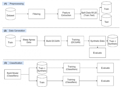
This research has three primary stages: preprocessing, data generation, and classification. The first stage is preprocessing consisting of filtering, feature extraction, and data splitting. The second stage is creating and training a DCGAN model to create synthetic data. The third stage is to classify and compare the results between performance before and after data augmentation (see Figure 1).
In the augmented data, the training data will be combined with the apnea data created using DCGAN. At the data generation and classification stages, the model's performance will be measured using several metrics, such as precision, recall, accuracy, F1-Score, and specificity for classification, and Root Mean Square Error (RMSE) and Fréchet Distance (FD) for data generation.
Figure 1. Proposed method
3.2.1 Filtering
At this stage, the dataset will be filtered. Filtering is done to remove the noise in the recording. Some examples of filters that can be used for ECG signals are in Table 1 [30].
Table 1. Types of ECG filters
|
Filter Name |
Frequency |
Description |
|
Bandpass |
5-11 Hz |
Remove noise in the raw signal |
|
Notch |
60 Hz |
Remove noise in the raw signal |
|
Bandpass second-order Butterworth filter |
5 and 35 Hz |
Remove noise in the raw signal |
|
Fourth-order low-pass zero-phase-shift Butterworth filter |
0.7 Hz |
Remove noise on the respiratory signal |
This study used a second-order Butterworth Bandpass filter with a frequency of 5 Hz lowpass and 35 Hz highpass. Here are the steps taken:
Figure 2. Comparison of the raw signal with the filtered one
Table 2. Example of labeling records data following labels from experts
|
Segments |
Apnea-ECG |
MIT-BIH |
Label |
|
Segment Length |
Segment Length |
||
|
Segment-1 |
0-5999 |
0-7499 |
N |
|
Segment-2 |
6000-11999 |
7500-14999 |
N |
|
. |
. |
. |
. |
|
. |
. |
. |
. |
|
Segment-N |
xxx-xxx |
xxx-xxx |
A or N |
After being divided into segments, there were 17062 and 10197 segments of Apnea-ECG and MIT-BIH. Then the segment will be divided into normal and apnea data based on the label. After the filtering process is complete, the feature extraction process will be done manually.
3.2.2 Feature extraction
The signal is divided into segments every minute and 30 seconds, filtered in the previous process, and then continued with feature extraction. Feature extraction is a method used to retrieve valuable information contained in the ECG signal that can represent the characteristics of apnea or not. Seven features will be taken from the ECG signal as described in Table 3.
Table 3. Extracted features
|
Feature |
Description |
|
Total peaks |
Total peaks per minute |
|
AvgHR |
Average heart rate per minute |
|
MeanNN |
The mean of the RR intervals. |
|
RMSSD |
The square root of the mean of the sum of successive differences between adjacent RR intervals. |
|
pNN50 |
The proportion of RR intervals greater than 50ms, out of the total number of RR intervals. |
|
Age |
Age of each patient |
|
Gender |
Gender of each patient |
$A v g H R=\sum_{h=1}^h \frac{1}{h}$ (1)
$MeanNN =\frac{\sum_{r=1}^{n_r} d_{r+1}-d_r}{n_r}$ (2)
$R M S S D=\sqrt{\frac{\left(d_{r r}\right)^2}{n_{r-1}}}$ (3)
$p N N 50=\left(\forall\left(n_r\right)(N N 50++) \leftarrow \sum_{r=1}^{n_r} d_{r+1}-d_r>50 \mathrm{~ms}\right) \times 100$ (4)
where, h=Number of heart rate, nr=Number of r peaks, NN50=$\left(\forall\left(n_r\right)(N N 50++) \leftarrow \sum_{r=1}^{n_r} d_{r+1}-d_r>50 m s\right)$, drr=$\sum_{r=1}^{n_r} d_{r+1}-d_r$.
The features ‘total peaks’, ‘avgHR’, ‘meanNN’, ‘RMSSD’, and ‘pNN50’ are taken from each segment. For ‘age’ and ‘gender’ are assigned to each segment according to the information in the dataset.
Table 4. DCGAN architecture
|
Generator |
Discriminator |
||||
|
Layers |
Size |
Activation |
Layers |
Size |
Activation |
|
BiLSTM |
16 |
- |
Conv1D |
7 |
LeakyReLu |
|
Conv1D |
32 |
LeakyReLu |
Dropout |
0.25 |
- |
|
Conv1D |
16 |
LeakyReLu |
Conv1D |
16 |
LeakyReLu |
|
Conv1D |
8 |
LeakyReLu |
Dropout |
0.25 |
- |
|
Dense |
7 |
Tanh |
Conv1D |
32 |
LeakyReLu |
|
|
|
|
Dropout |
0.25 |
- |
|
|
|
|
MaxPool1D |
2 |
- |
|
|
|
|
Dense |
1 |
Sigmoid |
3.2.3 Data splitting
The dataset that has been preprocessed is then divided into training data, validation data, and test data. Data distribution begins with a ratio of 60:20:20, where 60% are training data, 20% are validation data and 20% rest used for test data. Then this division scheme aims to separate test and validation data, so they are not mixed with synthetic data. Test data and validation data will be stored, then test data is used to test the model before and after augmentation, and validation data is used for tuning in the training process.
3.2.4 Data generation
For synthetic data generation, data from the training set will be taken from the unbalanced class (apnea class) and augmented to increase the data. And to make synthetic data almost resemble the original data from the ECG signal, a method that can imitate the original data is needed. The method used will be the Deep Convolution Generative Adversarial Network (DCGAN). In DCGAN, two deep network models (CNN, RNN, LSTM, etc.) will compete to find the best one.
3.2.5 Build DCGAN
DCGAN consists of two neural networks, Generator (G) and Discriminator (D), where these two models will compete to beat each other. The generator tries to learn from the distribution of the original data to create synthetic data like the original data. The primary purpose of the generator is to ‘fool’ the discriminator with the generated data. In contrast to the discriminator, the discriminator tries to detect which data is genuine and which is synthetic. The GAN model is said to be ‘deep’ because it uses three or more hidden layers. In constructing a stable GAN model, this study uses the guidance from Radford et al. [26], which claims to make training on the GAN more stable. Architectural guidelines for a stable Deep Convolutional GAN:
As can be seen in Table 4, the generator consists of a 4-layer (1 LSTM and 3 Conv1D) which receives 50 random samples that match the original data distribution with an output of 7x1 (7 features). Meanwhile, the discriminator consists of a 4-layer (3 Conv1D and 1 MaxPooling1D) with real or fake outputs. Then, the Adam optimizer is used to minimize the loss of the discriminator (5) and generator (6).
$D_{{loss }}=-\frac{1}{m} \sum_{i=1}^m log \left(D\left(x^i\right)\right)+log \left(1-D\left(G\left(\mathrm{z}^{\mathrm{i}}\right)\right)\right)$ (5)
$G_{ {loss }}=-\frac{1}{m} \sum_{i=1}^m log \left(1-D\left(G\left(z^i\right)\right)\right)$ (6)
where, m=number of samples per minibatch, x=real samples, z=noise vector / latent space, D=discriminator, G=generator.
3.2.6 Training DCGAN
After all the DCGAN architectural designs are ready, the next step is to train the model. Both models will be trained simultaneously using the apnea dataset only taken from the training data. The training process on the discriminator uses real data and synthetic data. This data is feed-forward, and the loss is calculated from the detection results. Next is backpropagation to adjust the weight of the discriminator.
Furthermore, the generator training begins by providing an input value as a random value. Then the generator tries to match the original data distribution to produce synthetic data that resembles the original data. The weights in the generator model are updated based on the performance of the discriminator model. When the discriminator can detect false data, the weights on the generator are updated more. When the discriminator model is relatively poor or confused when seeing fake data, the generator model is updated less. On DCGAN training, this study used the Adam optimizer on the second network, and the learning rate was 0.0002 [26]. A learning rate of 0.001 is considered too high and can cause failure in DCGAN training. The momentum used is 0.5, which can help stabilize DCGAN in the training process.
3.2.7 Join dataset (original + synthetic)
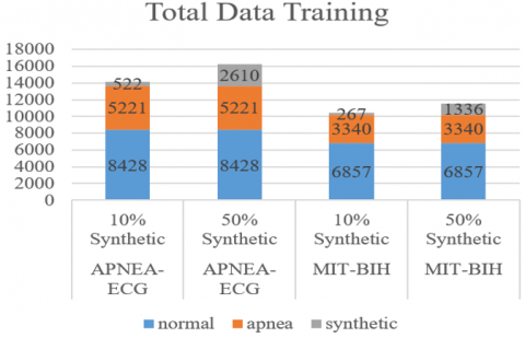
All data generated by DCGAN is then combined with the original dataset (see Figure 3). This merging process aims to add a minority class (apnea) with scenarios adding 10% and 50% of the original total apnea data.
Figure 3. Comparison of the amount of training data
3.2.8 Classification
The training data that has been split previously will be used to train the classifier model. The total training and testing data for Apnea-ECG were 13649 and 3413, respectively, and 5485 and 2672 for the MIT-BIH. Models considered suitable for sleep apnea data problems will be selected at this stage.
3.2.9 Build model (Classifier)
The model developed in this study is inspired by previous research, namely 1D-CNN from Almutairi et al. [20] and Wang et al. [21], by making minor modifications to some parameters. However, the results indicate that the model from Almutairi et al. is more suitable for preprocessed data in the previous stage, and it was decided to use this model. Three other classifier models are used for comparison, including ANN, LSTM, and 1D-CNN+LSTM.
(1) 1D-CNN (see Table 5): This 1D-CNN model was inspired by Almutairi et al. by increasing the number of layers, reducing neurons, and changing the kernel size to 2. This model removes the max-pooling layer and only uses the batch normalization layer after the convolution layer. Then use dropout on the last layer (before flattening).
(2) ANN (see Table 5): The ANN model was chosen because there are only eight input features, and it is considered suitable for performing simple tasks such as binary classification (normal and apnea). The ANN architecture has seven neurons in the input layer and one hidden layer with six neurons.
(3) LSTM (see Table 6): The LSTM model uses 64 neurons in the dense layer and 100 neurons in the LSTM layer, and 20% dropout.
(4) 1D-CNN+LSTM (see Table 6): The 1D-CNN+LSTM model uses the architecture of the previous 1D-CNN and is added to the LSTM layer.
Table 5. ANN and 1D-CNN architecture
|
ANN |
1D-CNN |
||||
|
Layers |
Size |
Activation |
Layers |
Size |
Activation |
|
Input |
7 |
ReLu |
Conv1D |
16 |
ReLu |
|
Hidden |
6 |
ReLu |
BatchNorm |
- |
- |
|
Dense |
1 |
Sigmoid |
Conv1D |
16 |
ReLu |
|
|
|
|
BatchNorm |
- |
- |
|
|
|
|
Conv1D |
32 |
ReLu |
|
|
|
|
BatchNorm |
- |
- |
|
|
|
|
Conv1D |
32 |
ReLu |
|
|
|
|
BatchNorm |
- |
- |
|
|
|
|
Conv1D |
64 |
ReLu |
|
|
|
|
BatchNorm |
- |
- |
|
|
|
|
Conv1D |
64 |
ReLu |
|
|
|
|
BatchNorm |
- |
- |
|
|
|
|
Dropout |
0.25 |
- |
|
|
|
|
Flatten |
- |
- |
|
|
|
|
Dense |
512 |
ReLu |
|
|
|
|
Dense |
256 |
ReLu |
|
|
|
|
Dense |
64 |
ReLu |
|
|
|
|
Dense |
1 |
Sigmoid |
3.2.10 Training (Before augmentation)
From Figure 4, it can be seen the amount of data between normal and apnea in the training data. There is an imbalance in the amount of data, whereas normal data is about 40% more. At this training stage, all models that have been built are trained using preprocessed data. The preprocessed training data is normalized into a range of [-1,1]. This study uses early stopping with a patience value of 5 to prevent overfitting for all models built using the Adam optimizer with an initial learning rate of 0.001 for 150 epochs.
Table 6. LSTM and 1D-CNN+LSTM architecture
|
LSTM |
1D-CNN+LSTM |
||||
|
Layers |
Size |
Activation |
Layers |
Size |
Activation |
|
Dense |
64 |
Dense |
Conv1D |
16 |
ReLu |
|
LSTM |
100 |
LSTM |
BatchNorm |
- |
- |
|
Dropout |
0.2 |
Dropout |
Conv1D |
16 |
ReLu |
|
BatchNorm |
- |
BatchNorm |
BatchNorm |
- |
- |
|
Flatten |
- |
Flatten |
Conv1D |
32 |
ReLu |
|
Dense |
64 |
Dense |
BatchNorm |
- |
- |
|
Dense |
1 |
Dense |
Conv1D |
32 |
ReLu |
|
|
|
|
BatchNorm |
- |
- |
|
|
|
|
Conv1D |
64 |
ReLu |
|
|
|
|
BatchNorm |
- |
- |
|
|
|
|
Conv1D |
64 |
ReLu |
|
|
|
|
BatchNorm |
- |
- |
|
|
|
|
Dropout |
0.25 |
- |
|
|
|
|
Flatten |
- |
- |
|
|
|
|
LSTM |
100 |
Tanh |
|
|
|
|
Dropout |
0.2 |
- |
|
|
|
|
BatchNorm |
- |
- |
|
|
|
|
Flatten |
- |
- |
|
|
|
|
Dense |
64 |
ReLu |
|
|
|
|
Dense |
1 |
Sigmoid |
Figure 4. Total training data (normal and apnea)
3.2.11 Training (After augmentation)
The same models and methods are used at this stage as in the stage before augmentation. All classifier models were rebuilt from scratch using the same parameters. However, the original training data has been combined with the synthetic data. The added synthetic data amounted to 10% and 50% of the total apnea training data. The effect of adding synthetic data will be seen and compared with before adding synthetic data.
In this experiment, this study uses four measurements—(i) precision, (ii) recall, (iii) f1-score, (iv) accuracy, and (v) specificity to see the performance of the model before and after augmentation. Since this is a binary classification, there will be two classes, positive and negative. When the predicted class of the sample matches the actual class, it is said to be True otherwise False. This study measures the four metrics based on True Positive (TP), True Negative (TN), False Positive (FP), and False Negative (FN) as follows:
Precision $=\frac{T P}{T P+F P}$ (7)
Recall $=\frac{T P}{T P+F N}$ (8)
$F 1- Score =\frac{2 \cdot { Precision } \cdot { Recall }}{{ Precision }+ { Recall }}$ (9)
$Accuracy =\frac{T P+T N}{T P+F P+T N+F N}$ (10)
$Specificity =\frac{T N}{T N+F P}$ (11)
The results in this study are divided into three, namely before augmentation, training results from DCGAN, and after augmentation. We use binary cross-entropy as the loss function for training before and after augmentation. Meanwhile, a custom loss function in DCGAN training is used in Eqns. (5) and (6) for the loss function. In the training process before and after augmentation, we used a batch size of 64 for all models; in DCGAN training, we used a batch size of 128. The test results before augmentation can be seen in Table 7, where 1D-CNN+LSTM and 1D-CNN got the best test accuracy, which is 80.49%, with 25 epochs for Apnea-ECG and 75.05% for MIT-BIH with 18 epochs.
Figure 5. Accuracy and loss (1D-CNN+LSTM)
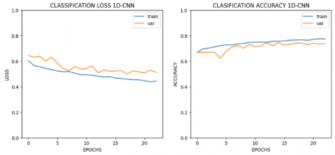
Figure 6. Accuracy and loss (1D-CNN)
The 1D-CNN+LSTM and 1D-CNN model at the stage before augmentation shows that the model is in the form of a ‘good fit’ (see Figures 5-6). The model is said to be a ‘good fit’ if the model can produce good accuracy on the test and validation data.
For DCGAN results, RMSE reflects the original and synthetic data stability. FD is used to measure the quality of the data generated by the GAN by looking at the similarity between the curves that take into the location and order of the points along the curve [31]. The smaller the FD value, the better the GAN’s generated data. RMSE and FD calculations as in Eqns. (12) and (13).
$R M S E=\sqrt{\frac{1}{N} \sum_{n=1}^N\left(x_{[n]^{-}} \hat{x}_{[n]}\right)^2}$ (12)
$F D(P, Q)=min \{/ / d / /\}$ (13)
x is a feature of the original data and $\widehat{x}$ is a feature of synthetic data. For FD, P is the sequence of data along the original data segment and Q is the sequence of data along the synthetic data segment. Where $\sigma(P)=\left(u_1, u_2, \ldots u_p\right)$ and $\sigma(Q)=\left(v_1, v_2, \ldots v_q\right)$, then we will get a sequence consisting of several points $\left\{\left(u_{a l}, v_{b_l}\right), \ldots\left(u_{a_m}, v_{b_m}\right)\right\}$. Length $\|d\|$ can be seen in Eq. (14).
$\|d\|=\max _{i=l, \ldots m} d\left(u_{a_l}, v_{b_l}\right)$ (14)
where, d represents Euclidean distance which basically has ai+1=ai or ai+1=ai+1 and bi+1=bi as requirements. From the results of our experiments, it was found that to produce a synthetic signal with a length of 6000 features (without manual feature extraction), the DCGAN often failed during training. Discriminators are sometimes too smart to detect which samples are real or synthetic.
Table 7. Results before augmentation
|
Model |
Dataset |
Pre (%) |
Rec (%) |
F1 (%) |
Spec (%) |
Epoch |
Acc (%) |
||
|
Train |
Val |
Test |
|||||||
|
1D-CNN |
APNEA-ECG |
78.35 |
78.93 |
78.59 |
81.39 |
14 |
78.76 |
78.73 |
79.49 |
|
MIT-BIH |
71.80 |
68.71 |
69.67 |
86.97 |
18 |
76.59 |
74.22 |
75.05 |
|
|
ANN |
APNEA-ECG |
71.69 |
72.14 |
71.87 |
76.09 |
32 |
73.78 |
74.3 |
73.04 |
|
MIT-BIH |
58.33 |
50.61 |
42.15 |
98.74 |
66 |
67.29 |
69.07 |
66.37 |
|
|
LSTM |
APNEA-ECG |
72.35 |
72.21 |
72.28 |
79.19 |
12 |
74.62 |
75.36 |
73.81 |
|
MIT-BIH |
63.6 |
58.09 |
57.73 |
89.82 |
30 |
69.76 |
68.63 |
69.17 |
|
|
1D-CNN+LSTM |
APNEA-ECG |
79.38 |
79.75 |
79.55 |
82.96 |
25 |
81.67 |
80.54 |
80.49 |
|
MIT-BIH |
69.84 |
68.89 |
69.29 |
82.24 |
13 |
74.38 |
72.35 |
73.38 |
|
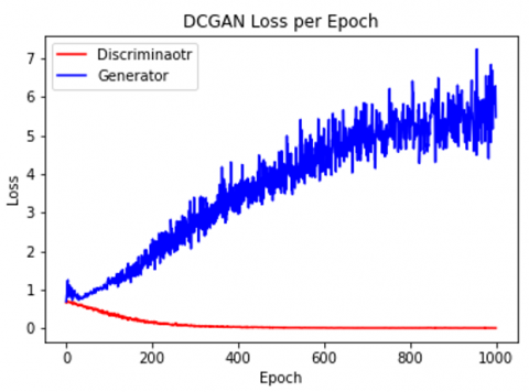
Therefore, to try stabilizing the DCGAN training, this study attempts to reduce the sample generated by manual feature extraction. The fewer features to be generated, the easier it is to stabilize the DCGAN training, as shown in Figures 7-8.
Figure 7. Loss DCGAN without feature extraction (6000 features)
Figure 8. Loss DCGAN with manual feature extraction (7 features)
It can be seen in Figure 8 that the loss is slightly erratic at the beginning of the training process and becomes stable around epoch 400. This is an example of normal loss during the DCGAN training process, where the two models will always compete until they reach a stable point. Using 7 features takes about 900 seconds to make training results faster than using 6000 features takes about 5200 seconds. To see the quality of the synthetic data generated, we took a sample of 10 generator models trained with several epochs. The results can be seen in Table 8.
From Table 8, the best overall DCGAN model was trained with 9000 epochs for Apnea-ECG and 7000 for MIT-BIH. RMSE and FD values are 0.36, 0.96 and 0.42, 1.21. The accuracy of the discriminator is between 48-52%, which means that the generator has a nearly 50% chance of fooling the discriminator with the data it generates. In Apnea-ECG, the DCGAN model reaches its best point at epoch 9000, which is longer when compared to MIT-BIH because the amount of data on Apnea-ECG is greater, so it requires more training.
The DCGAN model in the 9000th and 7000th epochs was used to create synthetic data to be added to the training data. After the synthetic data has been generated, the next step is to measure the impact of synthetic data on improving the performance of the deep learning model that has been created. There are two test scenarios, namely with the addition of 10% and 50% synthetic data compared with the previous model with training before augmentation.
Table 8. DCGAN evaluation
|
Epoch |
APNEA-ECG |
MIT-BIH |
||||
|
RMSE |
FD |
ACC (D) (%) |
RMSE |
FD |
Acc (D) (%) |
|
|
1000 |
0.46 |
1.38 |
0.49 |
0.55 |
1.49 |
0.50 |
|
2000 |
0.61 |
1.74 |
0.49 |
0.74 |
1.93 |
0.51 |
|
3000 |
0.53 |
1.44 |
0.49 |
0.55 |
1.49 |
0.51 |
|
4000 |
0.37 |
1.01 |
0.49 |
0.55 |
1.52 |
0.52 |
|
5000 |
0.36 |
0.99 |
0.48 |
0.65 |
1.86 |
0.51 |
|
6000 |
0.63 |
1.83 |
0.49 |
0.40 |
1.14 |
0.52 |
|
7000 |
0.46 |
1.23 |
0.49 |
0.42 |
1.21 |
0.48 |
|
8000 |
0.60 |
1.85 |
0.49 |
0.44 |
1.23 |
0.49 |
|
9000 |
0.36 |
0.96 |
0.48 |
0.61 |
1.56 |
0.50 |
|
10000 |
0.40 |
1.08 |
0.49 |
0.55 |
1.54 |
0.50 |
In Tables 11-12, data augmentation can improve some classification model performance. Improved performance can be seen in the numbers in bold. Model names in the table are represented using M1-M4 labels in the order of 1D-CNN, AND, LSTM, and 1D-CNN+LSTM. From the results of 10% augmentation, synthetic data only slightly improves the performance of the classification model because the dataset is still not balanced. Furthermore, the highest increase was obtained by the 1D-CNN+LSTM model for the Apnea-ECG dataset with an increase of 1.76%, and the LSTM model for the MIT-BIH dataset with a 4.80% increase in 10% augmentation.
Then, we found that a balanced or nearly balanced data set significantly affects the reliability of the deep learning model. Augmentation by 50% can improve the performance of the built model. Furthermore, for the test data, there was at least an increase of about 1% in all models for the Apnea-ECG dataset, with the most significant increase of 1.76% in the 1D-CNN model, and almost all models in the MIT-BIH dataset, with the most significant increase of 3.58% in the model LSTM. Then for precision, recall, f1-score, and specificity, almost all models can be improved. This proves that adding synthetic data to the dataset using DCGAN has increased the number of correct predictions for the apnea class.
We also compared DCGAN with other augmentation methods. This aims to prove that augmentation using DCGAN is better than augmentation methods such as SMOTE and ADASYN. Table 9 shows that the augmentation method with DCGAN is better than other augmentation methods. DCGAN can consistently improve model performance.
To see how well the model built in this study performed, we will take several references from previous research for comparison. Table 10 shows the effect of the unbalanced dataset handling technique. Sheta et al. [2], using the ADASYN technique to deal with data, proposed a study on imbalances. In the research conducted by Sheta et al., the proposed method is still unstable and only increases the precision. Compared with this study’s suggested results, it shows that DCGAN is better at handling data balance. DCGAN can improve accuracy, precision, and F1-Score to make the classification model more reliable. The classification model shown in the table is the best model taken from several models that have been tested.
Furthermore, this study also compares the overall performance of the proposed model with several models from previous studies in the classification of sleep apnea using manual feature extraction techniques.
Table 13 shows that the creation of synthetic data using the DCGAN model at least succeeded in increasing the performance of the classification model and could outperform models from several previous studies. The proposed method is better than Tripathi [23] and Mukherjee et al. [3] in terms of accuracy and recall. Using 7 features and data augmentation can perform better than previous studies.
Table 9. Comparison of testing accuracy DCGAN with other augmentation methods
|
Model |
Dataset |
No Aug |
SMOTE |
ADASYN |
DCGAN 50% |
|
M1 |
Apnea |
79.49 |
82.24 |
79.37 |
81.25 |
|
MIT-BIH |
75.05 |
71.62 |
68.73 |
76.32 |
|
|
M2 |
Apnea |
73.04 |
73.10 |
72.93 |
73.37 |
|
MIT-BIH |
66.37 |
61.96 |
61.03 |
66.18 |
|
|
M3 |
Apnea |
73.81 |
74.57 |
74.19 |
74.25 |
|
MIT-BIH |
69.17 |
62.84 |
66.96 |
72.75 |
|
|
M4 |
Apnea |
80.49 |
80.22 |
80.31 |
81.95 |
|
MIT-BIH |
73.38 |
70.49 |
69.12 |
74.95 |
Table 10. The effect of the technique handles data imbalance
|
Proposed Method |
Acc (%) |
Prec (%) |
F1 (%) |
|
Sheta et al. [2] – ensemble DT |
77.26 |
77.98 |
84.81 |
|
Sheta et al. [2] – ensemble DT (ADASYN) |
74.47 |
82.16 |
81.06 |
|
Our Proposed – 1D-CNN+LSTM |
80.49 |
79.38 |
79.55 |
|
Our Proposed – 1D-CNN+LSTM (DCGAN) |
81.95 |
80.92 |
81.03 |
Table 11. Comparison of no augmentation (0%) and with augmentation (10% and 50%) in Apnea-ECG
|
Model |
Pre (%) |
Rec (%) |
F1 (%) |
Spec (%) |
Test Acc (%) |
||||||||||
|
0% |
10% |
50% |
0% |
10% |
50% |
0% |
10% |
50% |
0% |
10% |
50% |
0% |
10% |
50% |
|
|
M1 |
78.35 |
79.71 |
80.29 |
78.93 |
79.6 |
79.94 |
78.59 |
79.65 |
80.10 |
81.39 |
84.63 |
85.68 |
79.49 |
80.75 |
81.25 |
|
M2 |
71.69 |
72.96 |
72.00 |
72.14 |
71.42 |
70.65 |
71.87 |
71.92 |
71.10 |
76.09 |
83.54 |
82.53 |
73.04 |
74.19 |
73.37 |
|
M3 |
72.35 |
71.51 |
72.95 |
72.21 |
71.94 |
73.46 |
72.28 |
71.68 |
73.15 |
79.19 |
76.00 |
76.9 |
73.81 |
72.87 |
74.25 |
|
M4 |
79.38 |
81.29 |
80.92 |
79.75 |
81.33 |
81.16 |
79.55 |
81.31 |
81.03 |
82.96 |
85.44 |
84.63 |
80.49 |
82.27 |
81.95 |
Table 12. Comparison of no augmentation (0%) and with augmentation (10% and 50%) in MIT-BIH
|
Model |
Pre (%) |
Rec (%) |
F1 (%) |
Spec (%) |
Test Acc (%) |
||||||||||
|
0% |
10% |
50% |
0% |
10% |
50% |
0% |
10% |
50% |
0% |
10% |
50% |
0% |
10% |
50% |
|
|
M1 |
71.80 |
71.74 |
73.06 |
68.71 |
71.1 |
72.52 |
69.67 |
71.39 |
72.77 |
86.97 |
82.89 |
83.47 |
75.05 |
75.20 |
76.32 |
|
M2 |
58.33 |
59.09 |
58.65 |
50.61 |
52.69 |
53.70 |
42.15 |
48.52 |
50.97 |
98.74 |
91.21 |
91.8 |
66.37 |
69.12 |
66.18 |
|
M3 |
63.60 |
70.57 |
68.89 |
58.09 |
68.96 |
64.80 |
57.73 |
69.57 |
65.67 |
89.82 |
86.11 |
87.57 |
69.17 |
73.97 |
72.75 |
|
M4 |
69.84 |
72.38 |
71.69 |
68.89 |
71.88 |
70.70 |
69.29 |
72.11 |
71.12 |
82.24 |
82.75 |
83.34 |
73.38 |
75.54 |
74.95 |
Table 13. Comparison of model performance using feature extraction with our proposed method (Apnea-ECG)
|
Proposed Method |
Features Used |
Acc (%) |
Rec (%) |
Spec (%) |
Window Size |
|
Tripathi [23] - KELM |
EDR and HRV |
76.37 |
78.02 |
74.64 |
- |
|
Feng and Liu [19] — SVM-HMM |
RRI |
84.70 |
68.80 |
94.50 |
6000x1 |
|
Mukherjee et al. [3]—Base model using Almutairi et al.’s CNN-LSTM |
RRI, RAMP and EDR |
84.08 |
82.94 |
86.15 |
240x3 |
|
Our Proposed—1D-CNN+LSTM (10% Augmentation) |
Total Peaks, Average Heart Rate, MeanNN, RMSSD, pNN50, Age, Gender |
82.27 |
81.33 |
85.44 |
7x1 |
|
Our Proposed—1D-CNN+LSTM (50% Augmentation) |
81.95 |
81.16 |
84.63 |
7x1 |
This study examines how data augmentation techniques using DCGAN can improve classification performance in deep learning and machine learning models. DCGAN can not only be implemented on data in the form of images but can also be used in the form of time series. This study found that data augmentation with DCGAN helps the classification model generalize better than other augmentation methods. The test results can increase the correct predictive value in the apnea class (TP) and decrease the incorrect predictive value in the apnea class (FN). Almost all models built and trained with the addition of synthetic data provide a performance increase, although not very large. Because no more information can make the classification model learn new patterns. This performance improvement also shows that the DCGAN model successfully generates synthetic data and imitates the distribution of the original data. This result is indicated by the relatively small RMSE and FD values and is close to 0, which means that it almost resembles the original data distribution. The highest increase was obtained by the 1D-CNN+LSTM model for the Apnea-ECG dataset with an increase of 1.76%, and the LSTM model for the MIT-BIH dataset with a 4.80% increase in 10% augmentation. Furthermore, for 50% augmentation, the highest accuracy increase was obtained by the 1D-CNN+LSTM model at 1.76% from the initial value of 80.49% to 81.95% for Apnea-ECG and almost all models in the MIT-BIH dataset, with the most significant increase of 3.58% in the model LSTM from an initial value of 69.17% to 72.75%. Future work could combine several public sleep apnea datasets for GAN training to provide various new information.
[1] Göğüş, F.Z., Tezel, G., Özşen, S., Küççüktürk, S., Vatansev, H., Koca, Y. (2020). Identification of apnea-hypopnea index subgroups based on multifractal detrended fluctuation analysis and nasal cannula airflow signals. Traitement du Signal, 37(2): 145-156. https://doi.org/10.18280/ts.370201
[2] Sheta, A., Turabieh, H., Thaher, T., Too, J., Mafarja, M., Hossain, M.S., Surani, S.R. (2021). Diagnosis of obstructive sleep apnea from ecg signals using machine learning and deep learning classifiers. Applied Sciences, 11(14): 6622. https://doi.org/10.3390/app11146622
[3] Mukherjee, D., Dhar, K., Schwenker, F., Sarkar, R. (2021). Ensemble of deep learning models for sleep apnea detection: An experimental study. Sensors, 21(16): 5425. https://doi.org/10.3390/s21165425
[4] Banluesombatkul, N., Rakthanmanon, T., Wilaiprasitporn, T. (2018). Single channel ECG for obstructive sleep apnea severity detection using a deep learning approach. In TENCON 2018-2018 IEEE Region 10 Conference, pp. 2011-2016.
[5] Nikolaidis, K., Kristiansen, S., Goebel, V., Plagemann, T., Liestøl, K., Kankanhalli, M. (2019). Augmenting physiological time series data: A case study for sleep apnea detection. In Joint European Conference on Machine Learning and Knowledge Discovery in Databases, pp. 376-399. https://doi.org/10.1007/978-3-030-46133-1_23
[6] Faust, O., Barika, R., Shenfield, A., Ciaccio, E.J., Acharya, U.R. (2021). Accurate detection of sleep apnea with long short-term memory network based on RR interval signals. Knowledge-Based Systems, 212: 106591. https://doi.org/10.1016/j.knosys.2020.106591
[7] Chaw, H.T., Kamolphiwong, S., Wongsritrang, K. (2019). Sleep apnea detection using deep learning. Tehnički Glasnik, 13(4): 261-266. https://doi.org/10.31803/tg-20191104191722
[8] Erdenebayar, U., Kim, Y.J., Park, J.U., Joo, E.Y., Lee, K.J. (2019). Deep learning approaches for automatic detection of sleep apnea events from an electrocardiogram. Computer methods and programs in biomedicine, 180: 105001. https://doi.org/10.1016/j.cmpb.2019.105001
[9] Rajawat, A.S., Mohammed, O., Bedi, P. (2020). FDLM: fusion deep learning model for classifying obstructive sleep apnea and type 2 diabetes. In 2020 Fourth International Conference on I-SMAC (IoT in Social, Mobile, Analytics and Cloud)(I-SMAC), pp. 835-839. https://doi.org/10.1109/I-SMAC49090.2020.9243553
[10] Hafezi, M., Montazeri, N., Saha, S., Zhu, K., Gavrilovic, B., Yadollahi, A., Taati, B. (2020). Sleep apnea severity estimation from tracheal movements using a deep learning model. IEEE Access, 8: 22641-22649. https://doi.org/10.1109/ACCESS.2020.2969227
[11] Zhang, G.Q., Cui, L., Mueller, R., Tao, S., Kim, M., Rueschman, M., Mariani, S., Mobley, D., Redline, S. (2018). The National Sleep Research Resource: Towards a sleep data commons. Journal of the American Medical Informatics Association, 25(10): 1351-1358. https://doi.org/10.1093/jamia/ocy064
[12] Blackwell, T., Yaffe, K., Ancoli-Israel, S., Redline, S., Ensrud, K.E., Stefanick, M.L., Laffan, A., Stone, K.L. (2011). Associations between sleep architecture and sleep-disordered breathing and cognition in older community-dwelling men: The osteoporotic fractures in men sleep study. Journal of the American Geriatrics Society, 59(12): 2217-2225. https://doi.org/10.1111/j.1532-5415.2011.03731.x
[13] Penzel, T., Moody, G.B., Mark, R.G., Goldberger, A.L., Peter, J.H. (2000). The apnea-ECG database. In Computers in Cardiology 2000. Vol. 27 (Cat. 00CH37163), pp. 255-258. https://doi.org/10.1109/CIC.2000.898505
[14] Chang, H.Y., Yeh, C.Y., Lee, C.T., Lin, C.C. (2020). A sleep apnea detection system based on a one-dimensional deep convolution neural network model using single-lead electrocardiogram. Sensors, 20(15): 4157. https://doi.org/10.3390/s20154157
[15] Almazaydeh, L., Elleithy, K., Faezipour, M. (2012). Detection of obstructive sleep apnea through ECG signal features. In 2012 IEEE International Conference on Electro/Information Technology, pp. 1-6. https://doi.org/10.1109/EIT.2012.6220730
[16] de Chazal, P., Penzel, T., Heneghan, C. (2004). Automated detection of obstructive sleep apnoea at different time scales using the electrocardiogram. Physiological Measurement, 25(4): 967. https://doi.org/10.1088/0967-3334/25/4/015
[17] Yılmaz, B., Asyalı, M.H., Arıkan, E., Yetkin, S., Özgen, F. (2010). Sleep stage and obstructive apneaic epoch classification using single-lead ECG. Biomedical Engineering Online, 9(1): 1-14. https://doi.org/10.1186/1475-925X-9-39
[18] Cheng, M., Sori, W.J., Jiang, F., Khan, A., Liu, S. (2017). Recurrent neural network based classification of ECG signal features for obstruction of sleep apnea detection. In 2017 IEEE International Conference on Computational Science and Engineering (CSE) and IEEE International Conference on Embedded and Ubiquitous Computing (EUC), Vol. 2, pp. 199-202. https://doi.org/10.1109/CSE-EUC.2017.220
[19] Feng, K., Liu, G. (2019). Obstructive sleep apnea detection based on unsupervised feature learning and hidden Markov model. In BIBE 2019; The Third International Conference on Biological Information and Biomedical Engineering, pp. 1-4.
[20] Almutairi, H., Hassan, G.M., Datta, A. (2021). Detection of obstructive sleep apnoea by ECG signals using deep learning architectures. In 2020 28th European Signal Processing Conference (EUSIPCO), pp. 1382-1386. https://doi.org/10.23919/Eusipco47968.2020.9287360
[21] Wang, X., Cheng, M., Wang, Y., Liu, S., Tian, Z., Jiang, F., Zhang, H. (2020). Obstructive sleep apnea detection using ECG-sensor with convolutional neural networks. Multimedia Tools and Applications, 79(23): 15813-15827. https://doi.org/10.1007/s11042-018-6161-8
[22] Sharan, R.V., Berkovsky, S., Xiong, H., Coiera, E. (2020). ECG-derived heart rate variability interpolation and 1-D convolutional neural networks for detecting sleep apnea. In 2020 42nd Annual International Conference of the IEEE Engineering in Medicine & Biology Society (EMBC), pp. 637-640. https://doi.org/10.1109/EMBC44109.2020.9175998
[23] Tripathy, R.K. (2018). Application of intrinsic band function technique for automated detection of sleep apnea using HRV and EDR signals. Biocybernetics and Biomedical Engineering, 38(1): 136-144.
[24] Hassan, A.R. (2016). Computer-aided obstructive sleep apnea detection using normal inverse Gaussian parameters and adaptive boosting. Biomedical Signal Processing and Control, 29: 22-30. https://doi.org/10.1016/j.bspc.2016.05.009
[25] Dey, D., Chaudhuri, S., Munshi, S. (2018). Obstructive sleep apnoea detection using convolutional neural network based deep learning framework. Biomedical Engineering Letters, 8(1): 95-100. https://doi.org/10.1007/s13534-017-0055-y
[26] Radford, A., Metz, L., Chintala, S. (2015). Unsupervised representation learning with deep convolutional generative adversarial networks. arXiv preprint arXiv:1511.06434.
[27] Mogren, O. (2016). C-RNN-GAN: Continuous recurrent neural networks with adversarial training. arXiv preprint arXiv:1611.09904.
[28] Zhu, F., Ye, F., Fu, Y., Liu, Q., Shen, B. (2019). Electrocardiogram generation with a bidirectional LSTM-CNN generative adversarial network. Scientific Reports, 9(1): 1-11. https://doi.org/10.1038/s41598-019-42516-z
[29] Ichimaru, Y., Moody, G.B. (1999). Development of the polysomnographic database on CD-ROM. Psychiatry and Clinical Neurosciences, 53(2): 175-177. https://doi.org/10.1046/j.1440-1819.1999.00527.x
[30] Mostafa, S.S., Mendonça, F., Ravelo-García, A.G., Morgado-Dias, F. (2019). A systematic review of detecting sleep apnea using deep learning. Sensors, 19(22): 4934. https://doi.org/10.3390/s19224934
[31] Zhu, F., Ye, F., Fu, Y., Liu, Q., Shen, B. (2019). Electrocardiogram generation with a bidirectional LSTM-CNN generative adversarial network. Scientific Reports, 9(1): 1-11. https://doi.org/10.1038/s41598-019-42516-z