Dhiyaa Salih Hammad* | Hamed Monkaresi
© 2022 IIETA. This article is published by IIETA and is licensed under the CC BY 4.0 license (http://creativecommons.org/licenses/by/4.0/).
OPEN ACCESS
Emotion detection from an ECG signal allows the direct assessment of the inner state of a human. Because ECG signals contain nerve endings from the autonomic nervous system that controls the behavior of each emotion. Besides, emotion detection plays a vital role in the daily activities of human life, where we lately witnessed the outbreak of the (COVID-19) pandemic that has a bad influence on the affective states of humans. Therefore, it has become indispensable to build an intelligent system capable of predicting and classifying emotions in their early stages. Accordingly, in this study, the Parallel-Extraction of Temporal and Spatial Features using Convolutional Neural Network (PETSFCNN) is established. So, in-depth features of the ECG signals are extracted and captured from the suggested parallel 2-channel structure of 1-dimensional CNN network and 2-dimensional CNN network and then combined by feature fusion technique for more dependable classification results. Besides, Grid Search Optimized-Deep Neural Network (GSO-DNN) is adopted for higher classification accuracy. To verify the performance of the proposed method, our experiment was implemented on two different datasets. The maximum classification accuracy of 97.56% and 96.34% on both valence and arousal were gained, respectively using the internationally approved DREAMER dataset. While the same model on the private dataset achieved 76.19% for valence and 80.95% for arousal respectively. The classification results of the PETSFCNN-GSO-DNN model are compared with state-of-the-art methods. The empirical findings reveal that the proposed method can detect emotions from ECG signals more accurately and better than state-of-the-art methods and has the potential to be implemented as an intelligent system for affect detection.
emotion detection, convolutional neural network (CNN), ECG signal, grid search optimization (GSO), DNN
Emotion is an intricate set of interactions of a human's psycho-physiological state that reflects his/her mood. As a result, emotional states can play a vital role in the daily activities of human life. And for emotional and valid interaction between human and computer, human emotion recognition is one of the essential stages that resulted in the advent of the field of affective computing (AC), which has become a hot topic in computer science and emotional intelligence for human-computer interaction [1, 2]. The field of affective computing aims to design systems that are capable of perceiving and expressing emotions [3]. We have recently noticed the COVID-19 pandemic spreading all over the world, especially in China. The peril of this pandemic caused not only fear of infection but also unbearable psychological stress [4]. During the COVID-19 pandemic, we also observed that most individuals were experiencing anxiety, stress, despair, loneliness, and fear. Thus, this will have a detrimental effect on a person's emotional well-being. Therefore, creating intelligent emotional recognition systems has become important in predicting such negative emotional states in the early stages, as well as it can provide assistance to clinicians in detecting and diagnosing mental disorders of people. In the last sixty years, the topic of human emotion has become researched increasingly across a wide range of domains, such as mental health care, e-learning, transportation companies, social security, and others. Human emotion recognition can be performed by recognizing facial expressions [5], body posture, speech tone [6, 7], and others. However, the physical signals [8] are easy to be camouflaged or hidden, it is hard to exclude the effect of individual factors, and it may be unable to recognize the inner true affective state. For example, a human might smile or pretend to be happy on a social occasion even if he/she is in a nonpositive affective state [9, 10]. Generally, we observed physiological signal-based emotion recognition has grown increasingly in the affective computing field [11]. Because physiological signals have several advantages over physical signals due to their sensitivity to inner emotions [12]. Therefore, physiological signals can show the inner emotions of the human without the tendency to hide or camouflage an affective state on social reasons [13].
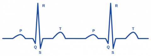
Currently, new methods and tools have been introduced by researchers and scholars to develop intelligent systems for detecting emotions in their early stages [14] as well as in the field of healthcare systems [15]. Building an accurate and reliable model has become important in detecting and recognizing human emotions via psychophysiological data [16]. Consequently, our study focuses specifically on emotion detection using ECG signals, because the neural cues can reflect human affective states more accurately and cannot be controlled or hidden by individual factors, so detecting and recognizing human affective states based on ECG cues has attracted scholars’ interest. ECG cues are the most commonly utilized compared to other cues because ECG contain-emotion related information [17, 18]. The ECG signal reflects the heart's electrical activity, non-invasive, and commonly utilized in a variety of applications. Figure 1 illustrates a typical depiction of the ECG signal.
Figure 1. The main components of an ECG signal include a P wave, a QRS complex, and a T wave
Furthermore, some of studies as in the study [19] used traditional machine learning techniques for classifying emotional states. In these studies, hand-crafted features extracted from ECG signals are typically applied as inputs to the classifiers. However, the performance of these features is limited by human expertise and the intricacy of classification problems. Due to those limitations, traditional methods cannot provide most daily human emotion recognition tasks. In recent years, human emotion recognition has made notable advances by using deep learning techniques to recognize human emotions. Instead of manual feature extraction and selection, deep learning makes it possible to extract and select features automatically. Compared to conventional machine learning techniques, feature extraction and classification tasks are usually conducted simultaneously in deep learning models.
Building an emotion recognition system based on ECG signals to accurately classify emotional states according to their levels in terms of low valence vs. high valence and low arousal vs. high arousal is a challenging task. To build such a model, several methodological issues need to be addressed such as feature extraction and classification task is among the most important issues that if are not addressed well, can hinder building a practical system.
The purpose of this research is to detect and classify ECG signals-based emotional states using convolutional neural networks (CNNs for feature extraction) and deep neural networks (DNNs for classification tasks). This study can be applied in several fields such as mental healthcare and to detect stress. Besides, in the classroom, detecting the negative affective states of students can help to enhance student learning experiences and improve their performance. In the area of transportation safety, recognizing various emotions such as anger, fatigue and stress can assist to issue an alert to the driver of a vehicle before a potential crash.
The main contributions of this paper are as follows:
The remainder parts of the paper are organized as follows. Section 2 presents background and related work. Section 3 describe the data and methods. Results and discussion are introduced in section 4. Lastly, section 5 provides the conclusion and future works of the proposed PETSFCNN-GSO-DNN model.
2.1 Dimensional model (valence - arousal model)
It is difficult to model or judge human emotions because individuals express their emotional states differently based on such factors as their subjective feeling and cognitive process. Over the past decades, several scholars have devoted to developing different emotion models for modelling human affective states. In the discrete models, users must select a specified list of word labels to tag/label emotional states in discrete categories for denoting their current emotion. Thereby, the stimuli may evoke mixed emotions that cannot be sufficiently expressed in words since the meanings of the selected words are culturally dependent. Thus, the discrete models need more than one word to specify blended emotions. While in the emotional dimensional models, individuals need to scale affective states in multiple dimensions for classifying emotions. Lately, two popular scales used for classifying emotions are valence and arousal planes. And most of the former studies have focused on using the 2D model to model emotions. So, rather than modeling emotional states of ECG signals as discrete emotions, they can be categorized by level of valence and arousal each (see Figure 2). For the aforementioned reasons, we applied the 2-dimensional Russell's model [20] to facilitate ECG-based emotion recognition. This model demonstrates that affective states are distributed in a 2D space with dimensions of valence and arousal. Valence plane indicates the horizontal axis and reflects the degree of pleasure that extends from highly negative to highly positive, while arousal plane represents the vertical axis and reflects the strength of emotional activity that ranges from low/passive to high/active.
Figure 2. Valence-arousal model/theory of emotions. X-axis denotes the valence plane, while Y-axis indicates the arousal plane
We can observe from Figure 2 how emotional states are categorized by this model. As we can also note that emotional states mapped in the lower-left quadrant are classified to be “Low Valence-Low Arousal”, whereas in the upper-right quadrant are categorized to be “High Valence-High Arousal”. Regarding the emotional states mapped in the lower-right quadrant are classified to be “High Valence-Low Arousal”, while in the upper-left quadrant are categorized as “Low Valence-High Arousal”. However, by determining the value of valence with arousal for some emotions, we can recognize affective states as four categories. In this study, the recognition task of emotional states is split into a binary classification method. This indicates that, the private and the DREAMER datasets are categorized in a two-category format by assigning a threshold at the average output value that divides the outputs into low and high. Thus, in our dataset, we split the rating scale of 1 to 9 into a binary classification method (low-high) with a threshold value of 5. While for the DREAMER dataset, we divided the rating scale of 1 to 5 into a binary classification method (low-high) with a threshold value of 3.
2.2 Related work
Therefore, several studies have been suggested to provide an ECG based detection system for classifying emotional states.
Among those studies, model selection is a challenging task facing most researchers in the field of affective computing (AC). Besides, feature extraction is also considered a challenging issue and represents a critical stage in the emotion classification.
In addition to the model/classifier selection, we have categorized the feature extraction frameworks for emotion detection into two main groups namely: (1) hand-crafted features, (2) automatic features.
The hand-crafted features need human expertise to extract useful information from ECG signals manually, which include different features such as (time-domain features, frequency domain features, time-frequency features, statistical features, and others). While regarding the automatic-extracted features, there is no need to extract features manually, where deep learning techniques such as convolutional neural networks (CNNs) can automatically extract robust features from raw ECG data. We reviewed different studies based on traditional and deep learning techniques that have been conducted in recent years, as presented below.
Subramanian et al. [21] proposed a Naive Bayes (NB) classifier for classifying emotional states. The authors used ASCERTAIN dataset that composed of 58 participants, and they used 36 emotive movie clips for eliciting affective states based on ECG signals. They also employed various features from ECG data such as frequency features and statistical features. The NB classifier achieved a classification accuracy of 60% and 59% for valence and arousal respectively. Wiem and Lachiri [22] suggested a support vector machine (SVM) classifier for detecting emotional states. They utilized MAHNOB database, which consisted of 24 subjects who participated in this experiment. The affective states were triggered using 20 video clips. Statistical features were extracted from ECG signals for recognizing affective states. The SVM classifier achieved a classification accuracy of 68.75% for valence emotions and 64.23% for arousal emotions. Hsu et al. [23] proposed a Least Squares SVM classifier to recognize and classify emotions based on ECG signals. The affective states were elicited using music from 61 subjects. Time-domain, frequency-domain, and nonlinear features were extracted from ECG signals. Thereafter, the LS-SVM classifier achieved a classification accuracy of 82.78% and 72.91% for both valence and arousal respectively. A study by Katsigiannis and Ramzan [24] introduced a SVM+RBF Kernel classifier for classifying emotional states. The classifier was applied to the DREAMER dataset that consisted of 23 subjects. Besides, the affective states were provoked using 18 various Audio-Video video clips. Heart Rate Variability (HRV) features and PQRST features were used in their proposed study. Finally, the SVM+RBF Kernel classifier attained a classification accuracy of 62.37% and 62.37% for valence and arousal respectively. Baghizadeh et al. [25] proposed a SVM-Polynomial and SVM-Linear for detecting human emotional states. Moreover, the researchers used time-domain, frequency-domain, time-frequency domain, and nonlinear features, afterward the SVM-Polynomial classifier attained a classification accuracy result of 78.07% for valence emotions, while the SVM-Linear achieved a classification accuracy of 82.17% for arousal emotions on the MAHNOB dataset.
In contrast to these five conventional methods for feature extraction, there is a deep learning technique. Deep learning (DL) is becoming an important method in bio-medical signal processing applications.
Santamaria-Granados et al. [26] proposed a developed deep convolutional neural network (DCNN) model for recognition of emotion. They obtained 75% and 76% results of classification accuracy for valence and arousal on the AMIGOS dataset that collected from 40 subjects, while they were watching 16 different video clips. Sarkar and Etemad [27] suggested and developed a self-supervised method based on a convolutional neural network (CNN). They achieved an average accuracy of 85% and 85.9% for both low/high valence and low/high arousal respectively on the DREAMER dataset. Finally, Harper and Southern [28] presented a developed CNN-LSTM model for classifying affective states based on ECG signals. On the DREAMER dataset, the CNN-LSTM model achieved a classification accuracy of 86% for low/high valence emotions.
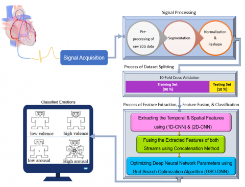
In this section, the proposed system for classifying emotional states using ECG signals includes five key tasks: datasets description, signal processing, feature extraction, feature fusion, and classification (see Figure 3). The introduced method is implemented and evaluated on two different datasets are as follows: 1- Private dataset; 2- Publicly available dataset known as the DREAMER database. So, the description of both datasets is presented in the next section.
3.1 Private dataset
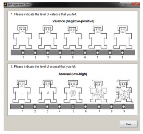
To detect emotions and to test the proposed model performance, we created a private dataset that was newly gathered from 23 subjects (fourteen male and nine female), aged between 20 and 60 years, while they viewed IAPS images. The emotional images were selected from the International Affective Picture System (IAPS) database, which gives a group of emotional stimuli to evoke emotions, and it is often used in the field of affective computing (AC). Therefore, the images of IAPS were utilized as visual stimuli for triggering thirteen diverse emotional states (calm, relaxed, content, glad, delighted, bored, annoyed, depressed, others, gloomy, afraid, angry, excited) from 23 subjects. So, after viewing each IAPS image, the subjects were asked to self-assess the emotions they felt by assigning values ranging from 1 to 9 to two different statuses are valence and arousal (see Figure 4, which shows the self-assessment form designed in MATLAB environment).
Figure 3. Block diagram of presented ECG-based emotion detection system
Figure 4. A snapshot for individual emotion rating
The private dataset is categorized in a two-category format by assigning a threshold at the average output value that divides the outputs into low and high. Thus, we split the rating scale of 1 to 9 into a binary classification method (low/high valence and low/high arousal) with a threshold 5. Besides, during the ECG cues recording, each subject was viewing 60 10-sec images for each, as well as a ten-sec gap between each viewed image which is still affected by the prior image. Therefore, the total time of each viewed image plus its related gap reached 20 sec. Figure 5 demonstrates the experimental protocol utilized for triggering the affective states. BIOPAC
MP150 system was used for recording ECG cues at a sampling rate of 1000 Hz by placing 2 electrodes on the wrists of the subject and one was placed on the left leg. In addition, two subjects were removed from the twenty-three subjects due to technical issues, which resulted in incomplete data. Therefore, recordings from 21 out of 23 subjects were utilized in this experiment. The overall period for recording ECG cues for each subject lasted nearly thirty minutes.
3.2 DREAMER dataset
DREAMER dataset [24] involves a recording of subject responses to audio-video content. Nine diverse affective states (calmness, excitement, fear, surprise, happiness, anger, amusement, sadness) were elicited from 23 subjects (14 M and 9 F), aged between 22 and 33 years. DREAMER dataset encompasses two physiological cues including ECG signal that contains 2-channels were sampled at 256 Hz using SHIMMER™ sensor [29]. For eliciting emotional states, 18 diverse (Audio-Video) clips were offered for each subject with a period lasting between (67-394 sec.). Moreover, baseline cues were also recorded as neutral cues (with no affect) before each stimulus clip with a period of 61 sec. On the other hand, the subjects used the self-assessment method from 1 to 5 for rating emotions. After that, the emotions were split into 2-classes by setting 3 as a threshold.
Figure 5. The empirical protocol used for eliciting emotional states using visual stimuli (IAPS images)
In this section, before the raw data are fed into the proposed system for detecting ECG-based emotion, they are required to be processed first according to the following steps:
4.1 Filtering
The second step filtered the ECG signal from noise and artifacts for both datasets. The ECG signal is typically contaminated by several types of noise, such as powerline interference and artifacts caused by body movements, respiration, and others which can affect extracting the information related to emotion from ECG signals. Therefore, it has become necessary to eliminate potential powerline interference and baseline drifts before being fed into the model for classifying affective states. As reported in the study [23], we filtered the ECG signal by applying two median filters, the first with a sliding window of length (600 ms) and the second with a sliding window of length (200 ms). Consequently, the resulting signal from the two median filters was passed to a (12-order) low pass filter with a cut-off frequency of (35 Hz) for removing the powerline interference resulted of the electrical network that ranges between (50 Hz - 60 Hz), as mentioned by Cuomo et al., and Berkaya et al. [30, 31].
4.2 Downsampling and segmentation
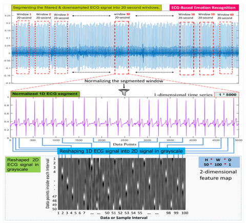
Concerning our dataset, the third step down-sampled the ECG signal to 250 Hz from 1000 Hz by a factor of 4 and then segmented it into 20-second windows with no-overlapping between the windows as depicted in Figure 6. Accordingly, the segmentation of the ECG signal resulted in 1260 chunks (21 subjects × 60 image) with a length of 5000 (20-sec × 250 Hz) data samples in each chunk ( $x \in \mathbb{R}^{5000}$ ) from 21 subjects.
Regarding the segmentation of the ECG signals of the DREAMER dataset, some of the studies use only the emotional signals without considering the impact of the neutral baseline signals (without emotional activity). ECG signals produced by the same participant under the same stimulations are often different due to the instability of human ECG signals and their sensitivity to some alternations in the surrounding environment. Therefore, in this study, we considered the baseline signals that were recorded through eighteen neutral video clips. As the neutral clips have no emotional activity was shown before each stimuli video clip (containing emotional activity) in order to help the participant, return to the neutral affective state. Whereas, these signals have proved their role and competence in improving the accuracy of emotion classification. Thus, these signals can be used as neutral signals to remove effects from the ECG signals while preserving the emotional content of the ECG data. To do this, we first must split the baseline signals and the experimental/emotional signals into chunks as follows:
1- In the first step we used N = 57-second of the baseline signals after omitting a 4-second out of 61-seconds of it.
2- In the second step we divided the 57-seconds of the neutral signals into 57 1-second chunks, then calculate the average of all chunks, as formulated in Eq. (1).
$\overline{B L}=\frac{\left(\sum_{n=1}^{N} B L_{n}\right)}{N}$ (1)
where, $\overline{B L}$ represents the mean of all the 57 chunks of 1-second each.
3- In the third step we used N=60-second of the emotional/experimental signals, which means that used the last 60-seconds of those signals.
4- In the fourth step we also divided the last 60-second of the emotional signals into 60 1-second segments $\left(E m o_{-} S e g_{i}\right)$.
5- In the fifth step we subtracted the mean value $\overline{B L}$ (computed in step 2) from each 1-second segment of the emotional signals mentioned in step 4, to get baseline removed segments and stack them in a matrix $\left(B L r_{S e g_{i}}\right)$, as indicated in Eq. (2).
$B L r_{-} S e g_{i}=\left(E m o_{-} S e g_{i}\right)-\overline{B L}$ (2)
Figure 6. The data segmentation, normalization and reshaping process
The aforementioned steps were intended to eliminate the neutral influences from ECG data while maintaining its emotional content. Eventually, the process of segmentation of the ECG signals resulted in 828 chunks (2-channels, 18-videos, 23-participants) with a length of 15360 samples each $\left(x \in \mathbb{R}^{15360}\right)$ (60-second each chunk × 256 Hz).
4.3 ECG segments normalisation
The next step after segmentation is the normalisation process. As aforementioned, there are a lot of factors that can impact the ECG signals such as the DC offset as well as the amplitude variance. To address such problems and to improve the quality of the ECG signals before being fed into the model, we have normalised and converted all the ECG data points to a common interval between [0,1] (Figure 6) through using the (min-max) normalisation method. The (min-max) method can be expressed as follows:
$X_{i}^{n}=\frac{X_{i}^{n}-X_{\min }}{X_{\max }-X_{\min }}$ (3)
where, $\left(X_{i}^{n}\right)$ represents the $\left(i^{t h}\right)$ data point of the $\left(n^{t h}\right)$ sample, while $\left(X_{\min }\right)$ and $\left(X_{\max }\right)$ denotes the minimum and maximum value of the $\left(n^{t h}\right)$ sample respectively.
4.4 ECG segments reshaping
Generally, 2D image signals contain more detailed and high-dimensional information, making them better for model generalisation, while real images have relatively redundant data. As a result, 1-dimensional ECG segments can be reshaped into a 2-dimensional gray-level map as an input to the model to decrease the adverse impacts. Thus, it improves the signal quality from noise comparatively as well as the utilisation efficiency of computing resources. Therefore, in this study, we have used both one and two-dimensional ECG signals as the input of our concurrent multi-channel model for their respective functions of representing various dimensions of information to improve the reliability of ECG data. Figure 6 depicts the process of normalising and reshaping ECG data that is segmented into 20-second windows. Regarding the normalised 1-dimensional ECG segments are kept as inputs to the 1D-CNN model for extracting temporal features. Meanwhile, according to the normalisation rule that the scaled samples values between 0 and 1 corresponding to the gray-level between (light = 0 and dark = 1), the 1-dimensional ECG segments are reshaped to create gray-level maps each. To do that, we take each 50 sample points of the normalised segment and stack them as the first column of the map, and so on to the remaining sample points. Thus, we will get a gray-level map of 100 columns each containing 50 grayscale color values corresponding to the sample points of the signal which were normalised between 0 and 1. Lastly, the generated gray level map can be fed as input to the 2D-CNN model for spatial features extraction.
4.5 Overview of the convolutional neural network (CNN)
This section provides a brief review of the most prominent deep learning methods, where the CNN algorithm is one of the common types of deep learning techniques based on artificial neural network structures, which can be 1-dimensional, 2-dimensional, or 3-dimensional. Generally, the traditional machine learning methods are composed of three different layers as follows: an input layer, one hidden layer, and an output layer, unlike the artificial neural network that has more than one hidden layer in its structure. Therefore, the artificial neural networks (ANNs) structure is inspired by the network of biological neurons of the brain working system that involves several hidden layers [32]. Each hidden layer includes many neurons that act as processing units for the inputs from other neurons in the previous layer, meaning that they provide a new representation of features that were extracted from the input data. The output of each neuron is calculated by the weighted sum of its inputs $\left(X_{i}^{l-1} \times W_{i j}^{l}\right)$), then adding a static value called bias propagated thru a nonlinear activation function as defined in Eq. (4) for the neuron activation and Eq. (5) for its output respectively.
$a_{j}^{l}\left(\boldsymbol{X}^{l-1}\right)=\sum_{i=1}^{N_{l-1}}\left(X_{i}^{l-1} \times W_{i j}^{l}\right)+b_{j}^{l}$ (4)
$X_{j}^{l}\left(\boldsymbol{X}^{l-1}\right)=\varphi\left(a_{j}^{l}\right)=\varphi\left(\sum_{i=1}^{N_{l-1}}\left(X_{i}^{l-1} \times W_{i j}^{l}\right)+b_{j}^{l}\right)$ (5)
where, $\left(X_{j}^{l}\right)$ represents the output of each neuron in the network at the $l$-th layer and the $j$-th index of the neuron within the layer, that obtains its inputs from all neurons in the earlier layer $\left(X_{i}^{l-1}\right), W_{i j}^{l}$ and $b_{j}^{l}$ are the neuron's weights and bias respectively, $\varphi$ indicates the neuron activation function.
Artificial Neural Networks (ANN) have been applied in several various fields such as computer vision, bioinformatics, natural language processing, and speech recognition, etc. Indeed, the CNNs is a type of artificial neural network, unlike the conventional neural network that cannot fully benefit from temporal or spatial features in the data.
In addition, the CNN network presents a new approach based on the spatially local connection and shared weights to integrate this information while considerably reducing the network complexity [33]. Therefore, the structure of the CNN network is essentially consisted of three main operations as follows: convolution, non-linearity and subsampling/pooling [34]. In short, CNNs can automatically extract and classify useful features from the input data using the operator of a convolution without the need for hand-learned features [35, 36]. As a result of which CNNs have gained a lot of interest in the visual field that includes images and videos.
Besides, the CNN algorithm is a feedforward network and it includes convolution layers, activation layers, and pooling layers. The principal functions of these layers are learning and extraction of robust features from the input data. Therefore, CNN is appropriate for addressing the problems of emotion detection from physiological signals and it is widely applied for learning and extracting optimal features from raw data, as well as classification tasks in different domains [37]. And to overcome the handcrafted features and to model the temporal and spatial structure in the ECG signals, 1D-CNN and 2D-CNN architectures are proposed in this research for ECG signals-based emotions classification.
4.6 The architecture of the proposed model
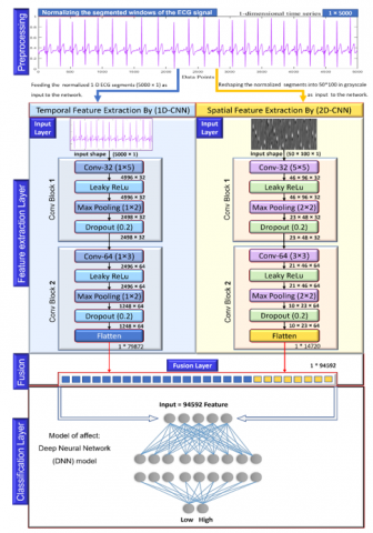
In this section, after performing the pre-processing steps of the ECG signals, the data are ready to be input into the PETSFCNN-GSO-DNN model, as depicted in Figure 8, which is based on deep learning (DL) techniques for classifying emotional states. Since the feature-learning process, which plays a significant role in classifying emotional states from ECG signals, is automated with CNNs, thus their use has become popular in this domain. Accordingly, the temporal and spatial features are extracted from ECG segments that have been normalized and reshaped with 2 parallel architectures, each of them containing convolutional, non-linearity, pooling, and dropout layers. Afterward, the outputs of both streams are first flattened, then fused using the concatenation method. Lastly, the GSO-DNN layer is followed to classify emotional states below.
4.6.1 Parallel-extraction of temporal and spatial features using convolutional neural network (PETSFCNN)
In this study, we proposed a novel end-to-end (PETSFCNN-GSO-DNN) model for detecting emotional states from ECG signals and classifying them according to the valence and arousal levels. The structure of the PETSFCNN-based feature extraction contains a parallel architecture of two types of CNNs are 1D-CNN for modeling temporal features and 2D-CNN for modeling spatial features. 1D-CNN is mainly used for modeling time-series or sequential data, which performs well in the extraction of their features [38]. For the above-mentioned reason, we have applied 1D-CNN for extracting temporal features. Besides, to extract more robust and useful features for classifying emotional states, we used 2D-CNN to extract spatial features from ECG signals after reshaping the 1-dimension ECG segments into a 2-dimensional gray-level map, as mentioned in part 3.2.4. The cause why we used 2D-CNN is that the two-dimensional convolution and pooling layers are convenient for filtering the spatial position of the 2D image signals. In extreme summary, convolutional neural networks extract deep features in both temporal and spatial dimensions of data, and thus, achieve a generalization performance for detecting emotions using physiological cues.
Finally, the architecture of the proposed model for extracting ECG features consists of two networks, as mentioned before. But for more information about the two networks, we have explained them in detail as follows. The first network is a 1D-CNN which is consisted of 2 convolutional blocks. The first block includes one convolutional layer composed of 32 kernels of size (1×5), followed by an activation function layer of type (Leaky ReLu), a max-pooling layer of size (1×2), and a dropout layer with a drop-rate (0.2). While the second block contains the same as the previous layers, except for the number of filters in the convolutional layer is increased to 64 filters of size (1×3), with adding a new flatten layer to it at the end. The 2D-CNN is the second network that has the same structure as the 1D-CNN network, but the only difference between them is, for example, that instead of being the kernel size is (1×m) will be (m×n). Both networks include the following layers:
(1) Convolution layer
Each 1-dimensional convolutional layer contains several feature maps, where each feature map consists of many neurons. Thus, the ECG signals in each convolutional layer are subjected to a 1-dimensional convolution filter/s to extract emotional features from those signals. Therefore, the extracted feature maps using 1-D convolution can be expressed as:
$F_{j}^{l}=\sum_{i=1}^{m}\left(X_{i}^{l-1} \bigotimes K_{i j}^{l}\right)+b_{j}^{l}$ (6)
where, $\otimes$ indicates the convolution operator, $F_{j}^{l}$ denotes the outputted feature map by $j$-th convolutional filter within the $l$-th layer, which obtains its input from the prior layer $\left(X_{i}^{l-1}\right)$, $K_{i j}^{l}$ and $b_{j}^{l}$ are the filter's weights and bias respectively, $m$ represents the size of the input vector in $X^{l-1}$. Likewise, the 2D convolution process can be calculated by:
$F_{i j}^{l}=\sum_{m=1}^{p} \sum_{n=1}^{p}\left(X_{(i+m, j+n)}^{l-1} \otimes K_{m n}^{l}\right)+b_{i j}^{l}$ (7)
where, each feature $F_{i j}^{l}$, acquired from multiplying $X_{(i+m, j+n)}^{l-1}$ which indicates the spatial location of the feature map at the previous layer $(l-1)$ with the $K_{m n}^{l}$ that represents the convolutional kernel/filter at layer $(l)$ with size $(p * p)$, then summed. Hence, the volume of feature maps can be calculated as defined Eq. (8):
Output $=\left(\frac{I-K+2 * \text { Padding }}{\text { Stride }}\right)+1$ (8)
where, I denotes the input size, K indicates the kernel/filter size.
(2) Activation function layer
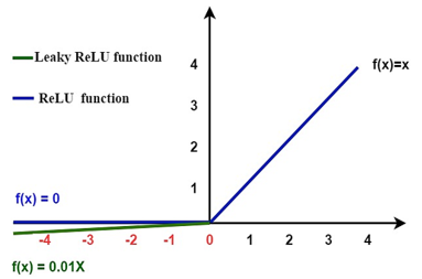
The activation function increases or improves the network's nonlinearity [39]. And since the output of each convolutional layer is a linear computation process. Therefore, a non-linear activation is added to the linear action. Thus, the outputted feature map from convolutional layer is passed through an activation function of type leaky rectified linear unit (LeakyReLU). It is notable that the use of LeakyReLU activation after each convolutional output instead of using ReLU activation is for addressing the dying ReLU problem for negative values. The function of the LeakyReLU operation is displayed in Eq. (9).
$F_{j}^{l}=\varphi\left(X_{i}^{l-1}\right)=\max \left(\alpha * X_{i}^{l-1}, X_{i}^{l-1}\right)$,
$\max \left(\alpha * X_{i}^{l-1}, X_{i}^{l-1}\right)= \begin{cases}X_{i}^{l-1}, & \text { if } X_{i}^{l-1}>0 \\ \alpha * X_{i}^{l-1}, & \text { otherwise }\end{cases}$ (9)
where, $\varphi$ indicates the (LeakyReLU) activation function and $\alpha$ stands for a small value called alpha which was set to $(\alpha=0.01)$. It is necessary to note that applying a (LeakyReLU) function decreases the death of neurons in the network when the input $X^{l-1}<0$, which means that the output of LeakyReLU will have a small negative slope of $(\alpha=0.01)$ in contrast to the ReLU function the output will be zero. Figure 7 shows the difference between the Leaky ReLU and ReLU function [40].
Figure 7. Visualizing the LeakyReLU and ReLU functions
(3) Pooling/downsampling layer
Thereafter, the outputted features from the previous layer are passed into the pooling layer or so-called subsampling layer. The pooling layer performs downsampling based on local connection to decrease unnecessary data while keeping the beneficial information. The features generated by the max-pooling function can be defined as:
$F_{i j}^{l}=\max \left(f_{(i-1) 1+k,(j-1) 1+k}^{l-1}, \ldots, f_{k i,(j-1) 1+k}^{l-1}, \ldots\right.$,
$\left.f_{(i-1) 1+k, k j}^{l-1}, \ldots, f_{k i, k j}^{l-1}\right)$ (10)
where, $F^{l}$ is the output feature at layer 1 that derived from the previous layer $F^{l-1}$, here $\mathrm{k} \times \mathrm{k}$ denotes the spatial region size, and $(1 \leq i, j \leq(p-q+1) / k), \mathrm{p}$ represents the input size of feature map, and q refers to the kernel/filter size. Anyway, the max function simply decreases the input features within the spatial region based on the maximum value.
(4) Dropping layer
One of the most prominent obstacles in deep models is overfitting. And to increase the model’s generalization and regularization better, the dropout method is used. As some of the neurons randomly will be ignored during the training process according to a given ratio called dropout rate. Thus, the dropout operation [41] not only protects or prevents the model from over-fitting but also speeds up the model's performance. The dropout operation can be formulated as follows:
Dout $=\operatorname{dropout}\left(F_{i j}^{l}\right)$ (11)
4.6.2 Feature flattening strategy
As can be seen from the 1D-CNN network (Figure 8), the overall number of temporal features extracted from input data was 79872 ( $F^{T} \in \mathbb{R}^{79872}$ ). Whereas from the 2D-CNN network, the total number of spatial features extracted from input data was 14720 ( $F^{S} \in \mathbb{R}^{14720}$ ). Anyhow, the next step after extracting features is the flattening operation, which reshapes the different dimensions to have a 1-D shape. Therefore, the 2-D data must be flattened into a 1-D vector before being fused with the temporal features. For example, the flattening process can be expressed as:
$A_{i}^{S}=\left[\begin{array}{ccc}f_{11} & \cdots & f_{1 w} \\ \vdots & \ddots & \vdots \\ f_{h 1} & \cdots & f_{h w}\end{array}\right]=\left[\begin{array}{cc}1 & 2 \\ 3 & 4 \\ 5 & 6\end{array}\right]$ (12)
$F_{i}^{S}=\operatorname{flatten}\left(A_{i}^{S}\right)=\left[f_{11}, \ldots, f_{1 w}, \ldots, f_{21}, \ldots\right.$,
$\left.f_{2 w}, \ldots, f_{h 1}, \ldots, f_{h w}\right]=\left[\begin{array}{cccccc}1 & 2 & 3 & 4 & 5 & 6\end{array}\right]$ (13)
where, $A_{i}^{S}$ is a $2 \mathrm{D}$ spatial feature map of size hight $\times$ width; $f$ refers to the value of the feature. $F_{i}^{S}$ represents the flattened spatial features as a $1-\mathrm{D}$ vector.
4.6.3 Feature fusing strategy
After the temporal and spatial features are extracted and then flattened to vectors, they must be fused before being passed to the DNN model for detecting emotions. It is clear from Figure 8 and Table 1 that the feature fusion strategy is an intermediate level fusion in between the data level and decision level. It can prevent a large amount of computation and loss of information. Thus, to improve the performance of the proposed model for detecting and classifying emotions with high accuracy, the flattened features of both streams are fused using the concatenation strategy as described below:
$C F_{i}^{T} \in \mathbb{R}^{1 \times 94592}=\left(F_{i}^{T} \in \mathbb{R}^{1 \times 79872}\right) \oplus\left(F_{i}^{S} \in \mathbb{R}^{1 \times 14720}\right)$ (14)
where, $\bigoplus$ represents the concatenation operator, $C F_{i}^{T}$ refers to the total size of the concatenated features of both streams with a length of 94592 samples, $F_{i}^{T}$ is the size of the extracted temporal features with a length of 79872 samples, while $F_{i}^{S}$ denotes the size of the extracted spatial features with a length of 14720 samples. The model can get more inclusive and precise evaluation findings, by flattening and fusing the temporal and spatial features to a joint vector.
Figure 8. The architecture of the PETSFCNN-GSO-DNN model for detecting emotions
Table 1. The layer properties of the performed (PETSFCNN-GSO-DNN) model
|
Layer name |
Kernel |
Kernel-Size |
Stride |
Padding |
Drop-Rate |
Output Shape |
Param # |
|
|
1D-CNN: |
|
|
|
|
|
|
|
|
|
Input layer-1 |
- |
- |
- |
- |
- |
5000 × 1 |
0 |
|
|
Conv1D 1-1 |
32 |
1 × 5 |
1 |
valid |
- |
4996 × 32 |
192 |
|
|
Leaky-ReLu 1-1 |
- |
- |
- |
- |
- |
4996 × 32 |
0 |
|
|
Max-Pooling1D 1-1 |
- |
1 × 2 |
2 |
valid |
- |
2498 × 32 |
0 |
|
|
Dropout 1-1 |
- |
- |
- |
- |
0.2 |
2498 × 32 |
0 |
|
|
Conv1D 1-2 |
64 |
1 × 3 |
1 |
valid |
- |
2496 × 64 |
6208 |
|
|
Leaky-ReLu 1-2 |
- |
- |
- |
- |
- |
2496 × 64 |
0 |
|
|
Max-Pooling1D 1-2 |
- |
1 × 2 |
2 |
valid |
- |
1248 × 64 |
0 |
|
|
Dropout 1-2 |
- |
- |
- |
- |
0.2 |
1248 × 64 |
0 |
|
|
Flatten-1 |
- |
- |
- |
- |
- |
1 × 79872 |
0 |
|
|
|
|
|
|
|
|
|
|
|
|
2D-CNN: |
|
|
|
|
|
|
|
|
|
Input layer-2 |
- |
- |
- |
- |
- |
50 × 100 × 1 |
0 |
|
|
Conv2D 2-1 |
32 |
5 × 5 |
1 |
valid |
- |
46 × 96 × 32 |
832 |
|
|
Leaky-ReLu 2-1 |
- |
- |
- |
- |
- |
46 × 96 × 32 |
0 |
|
|
Max-Pooling1D 2-1 |
- |
2 × 2 |
2 |
valid |
- |
23 × 48 × 32 |
0 |
|
|
Dropout 2-1 |
- |
- |
- |
- |
0.2 |
23 × 48 × 32 |
0 |
|
|
Conv2D 2-2 |
64 |
3 × 3 |
1 |
valid |
- |
21 × 46 × 64 |
18496 |
|
|
Leaky-ReLu 2-2 |
- |
- |
- |
- |
- |
21 × 46 × 64 |
0 |
|
|
Max-Pooling2D 2-2 |
- |
2 × 2 |
2 |
valid |
- |
10 × 23 × 64 |
0 |
|
|
Dropout 2-2 |
- |
- |
- |
- |
0.2 |
10 × 23 × 64 |
0 |
|
|
Flatten-2 |
- |
- |
- |
- |
- |
1 × 14720 |
0 |
|
|
Fusion-layer: |
|
Concatenation of (1 × 79872) & (1 × 14720) into 1×94592 |
0 |
|||||
|
Classification-layer: |
|
GSO-DNN classifier |
|
|||||
|
FC-layer 1-1 |
128 |
- |
- |
- |
- |
1 × 128 |
12107904 |
|
|
Leaky-ReLu 1-1 |
- |
- |
- |
- |
- |
1 × 128 |
0 |
|
|
Batch-Norm 1-1 |
- |
- |
- |
- |
- |
1 × 128 |
512 |
|
|
Dropout 1-1 |
- |
- |
- |
- |
0.2 |
1 × 128 |
0 |
|
|
FC-layer 1-2 |
64 |
- |
- |
- |
- |
1 × 64 |
8256 |
|
|
Leaky-ReLu 1-2 |
- |
- |
- |
- |
- |
1 × 64 |
0 |
|
|
Batch-Norm 1-2 |
- |
- |
- |
- |
- |
1 × 64 |
256 |
|
|
Dropout 1-2 |
- |
- |
- |
- |
0.2 |
1 × 64 |
0 |
|
|
Output = FC-SoftMax |
2 |
- |
- |
- |
- |
1 × 2 |
130 |
|
Figure 9. Hyper-parameter optimization of DNN model using GSO algorithm
Table 2. The hyper-parameters of DNN classifier are tuned automatically using Grid Search Optimization (GSO)
|
Parameters |
Values of hyper-parameters |
Selected parameters values |
|
No. of neurons in layer_1 |
[32, 64, 128] |
128 |
|
No. of neurons in layer_2 |
[32, 64, 128] |
64 |
|
Epoch |
[50, 100, 150] |
50 |
|
Activation function |
[‘ReLu’, ‘LeakyRelu’] |
‘LeakyRelu’ |
|
Dropout Rate |
[0.2, 0.5] |
0.2 |
|
Learning Rate |
[1e-2, 1e-3] |
1e-3 |
|
Batch size |
[64, 128] |
128 |
Notes: LeakyRelu means a Leaky Rectified Linear Unit, Adam means an Adaptive Moment Estimation
4.6.4 GSO-DNN classifier
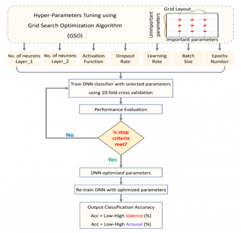
After extracting and fusing features process, the next stage is the classification process. Therefore, the final vector of the fused features is passed into the GSO-DNN model, which consists of two fully connected (FC) layers with 128 and 64 neurons each. Therefore, each fully connected layer is followed by an activation layer of type LeakyReLU, batch normalization layer, and dropout layer with a dropout rate of 0.2. Besides, to overcome and reduce the over-fitting problem, grid search optimization (GSO) algorithm is used for optimizing/tuning the hyper-parameters of the DNN model. The tuned parameters of the DNN model are presented in Table 2 and depicted in Figure 9. Lastly, the output layer of the DNN classifier consists of two neurons, where the first one represents low valence and the second one represents high valence (low arousal and high arousal), as showed in Figure 8 (classification layer). The activation function utilized with the output layer is the softmax function which can forecast the probability of the target class, as defined below:
$\operatorname{Softmax}\left(X_{j}\right)=\frac{e^{X_{j}}}{\sum_{i=1}^{n} e^{X_{j}}}, i=1,2, \ldots, n$ (15)
where, $X_{j}$ represents the input vector of the fused features, n indicates the number of emotional classes in the last layer. As the classification problem in this study is a binary classification task, therefore n=2. Furthermore, the loss function utilized in the output layer is based on the cross-entropy loss (CEL) function as defined in Eq. (16):
$C E L=-\sum_{i=1}^{C} L_{i} \times \log \left(X_{j}\right)$ (16)
where, $c$ is the number of emotional classes, $L_{i}$ indicates the (ground-truth label), and $X_{j}$ denotes the predicted label.
4.6.5 Implementation and evaluation metrics of the proposed method
For implementing the programming code of our experiment, we utilized the GPU of Google Colab via a laptop with the following specification: windows 10 Pro 64-bit, Intel(R) Core (TM) i7-4600U CPU @ 2.10GHz, 256-GB SSD, 12-GB DDR3 RAM. There are different methods utilized for reserving any data set as (training and test) data. This study suggests using the k-fold cross-validation strategy with k = 10 for dividing the dataset into training and testing sets. k-fold cross validation strategy is a resampling method used to reduce variance, bias, and errors in the dataset as well as aids to avoid overfitting problems and improves the performance of the model in terms of accuracy and stability. Therefore, 90% of the dataset was selected randomly for training the model and 10% for testing its performance (this operation is repeated ten times) [27]. The average of the ten test results is calculated to obtain the model's final efficiency. Besides, different metrics were used such as accuracy, F1-score, sensitivity, specificity, receiving operating characteristic (ROC) curve, and confusion matrix. All the above-mentioned metrics can be computed by four parameters in confusion matrix: TP is the true positive, TN is the true negative, FP is the false positive, and FN is the false negative. The equations for these metrics are presented as follows:
$\operatorname{Accuracy}(\%)=\frac{(T P+T N)}{(T P+T N+F P+F N)} \times 100$ (17)
$\operatorname{recision}(\%)=\frac{T P}{T P+F P} \times 100$ (18)
$\operatorname{Sensitivity}(\%)=$ Recall $=\frac{T P}{T P+F N} \times 100$ (19)
Specificity $(\%)=\frac{T N}{T N+F P} \times 100$ (20)
$F 1-\operatorname{Score}(\%)=2 \times \frac{(\text { Recall }) \times(\text { Precision })}{(\text { Recall })+(\text { Precision })}$ (21)
$C . M=\left[\begin{array}{cc}T N & F p \\ F N & T P\end{array}\right]$ (22)
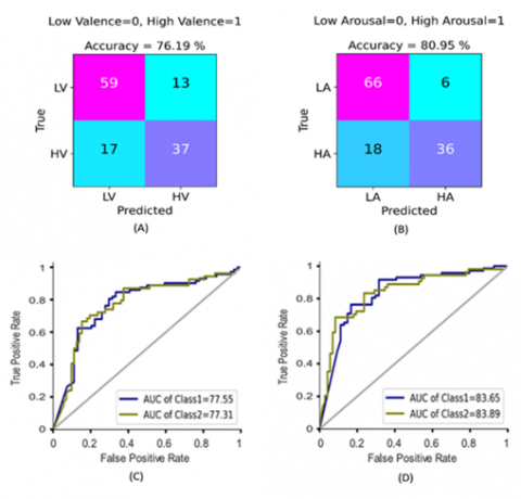
This section presents the experimental findings of the proposed PETSFCNN-GSO-DNN model. The efficiency of automatically extracted temporal and spatial features of ECG signals was investigated on two datasets, the first is a private dataset, and the second is a freely available DREAMER dataset. The PETSFCNN-GSO-DNN model achieved the highest classification accuracy and F1-score on the private dataset of 76.19% and 75.65% for emotional low/high valence, respectively, whereas achieved a classification accuracy of 80.95% and F1- score of 80.01% for emotional low/high arousal, respectively. The same model was applied and evaluated over the DREAMER dataset for recognition of emotional low/high valence and emotional low/high arousal. The proposed model obtained an average accuracy and F1-score over the DREAMER dataset of 97.56% and 97.30% for classifying the emotional states of low/high valence, respectively, whereas it attained an average accuracy of 96.34% and F1-score of 94.74% for classifying the emotional states of low/high arousal. Besides, the empirical results of the proposed model were presented in Table 3 for both datasets. Regarding the private dataset, Figure 10 shows the confusion matrices (A) and (B) of the test set for the GSO-DNN classifier for classifying emotional states as two (low and high) classes of both valence and arousal respectively.
Concerning the confusion matrix of emotional valence, we can see from Figure 10 (A) that among 126 affective states, 44 were misclassified by the GSO-DNN classifier, with 23 and 21 affective states for each of low valence and high valence respectively. Besides, the classification results show that the class of high valence attained better results as compared to the class of low valence. In the case of emotional arousal class, from Figure 10 (B), we can observe that among 126 emotional states, 24 affective states were incorrectly classified by the GSO-DNN classifier, with 6 and 18 affective states for each of low arousal and high arousal respectively. It should be noted that the class of low arousal attained better results than the class of high arousal.
Besides, the ROC curves of the GSO-DNN classifier on the test set are located between the recall/sensitivity (Eq. (19)) and false positive rate as demonstrated in Figure 10 (C) and (D). The average result of the area under the ROC curve was computed to be 77.43% and 83.77% for both valence and arousal respectively. For the DREAMER dataset, the same GSO-DNN classifier was implemented on it separately. Figure 11 demonstrates the confusion matrices (A) and (B) of the test set for the GSO-DNN classifier for classifying emotional states as two (low and high) classes of both valence and arousal respectively.
Figure 10. The tested GSO-DNN classifier on the private dataset: Confusion matrices (A), (B) and ROC curves (C), (D) with AUCs for classifying two categories (low-high) for each of valence and arousal respectively for the test set
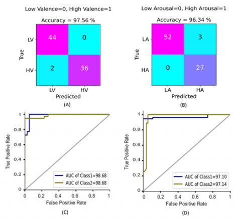
Regarding the confusion matrix of emotional valence, we can see from Figure 11 (A) that among 82 affective states, two were misclassified by the GSO-DNN classifier, with 0 and 2 affective states for each of low valence and high valence respectively. Besides, the classification results show that the class of low valence attained better results as compared to the class of high valence. In the case of emotional arousal class, from Figure 11 (B), we can see that among 82 emotional states, three affective states were incorrectly classified by the GSO-DNN classifier, with 3 and 0 affective states for each of low arousal and high arousal respectively. It should be noted that the class of low arousal attained better results than the class of high arousal. As shown in Figure 11 (C) and (D), the average finding of the AUCs was computed to be AUC =98.68% for valence and AUC =97.12% for arousal.
Figure 11. The tested GSO-DNN classifier on the DREAMER dataset: Confusion matrices (A), (B) and ROC curves (C), (D) with AUCs for classifying two categories (low-high) for each of valence and arousal respectively for the test set
In the last years, ECG-based emotion detection has become a hot topic in the area of affective computing, and several scholars have presented various classification methods to obtain good results. But the need still exists to find more efficient methods to recognize and classify affective states based on ECG data.
However, some challenges still exist in the field of affective computing, where most machine learning methods need handcrafted features before being fed into classifiers. Therefore, these methods not only limit the performance of the classifiers but also need human expertise to extract useful features from ECG signals. Thus, our proposed study aims to find a more efficient method to detect emotional states from ECG signals. And to overcome such aforementioned limitations, we proposed and developed a new method to parallelly extract the temporal and spatial features from ECG signals using CNN models, then the extracted features were fused and fed into the DNN model for detecting human emotional states. It should be also noted that our proposed method has achieved better results than the state-of-the-art studies. The reasons that resulted in obtaining higher results than the related studies are feature extraction, feature fusion, and optimization DNN model.
Table 3. Classification results (%) of PETSFCNN-GSO-DNN model on two datasets
|
Datasets |
Signals |
Stimulus |
Valence Arousal |
|||
|
Accuracy (%) |
F1-score (%) |
Accuracy (%) |
F1-score (%) |
|||
|
Private |
ECG |
IAPS |
76.19 |
75.65 |
80.95 |
80.01 |
|
DREAMER |
ECG |
Audio-Visual |
97.56 |
97.30 |
96.34 |
94.74 |
To establish a fair comparison with the related studies, we compared the performance of the proposed method with those methods [24, 27, 28] based on the DREAMER dataset. Beside we can observe from Table 4 that the proposed PETSFCNN-GSO-DNN model outperforms better than all the state-of-the-art studies in detecting and classifying emotional states.
Furthermore, Table 4 explains the comparison of the works mentioned previously in this study between used methods and their classification results, including F1-score if any. Besides, based on the results presented in Table 4, we can conclude the advantages of our proposed method are below:
1) The proposed method is a reliable and accurate computer-aided system in emotion detection which presents ideal average classification accuracy of 97.56% and 96.34% for valence and arousal, and the F1-score value of 97.30% and 94.74% for valence and arousal on the DREAMER dataset, where this refers to the effectiveness of binary classification.
2) The proposed method has the possibility to extracts useful and robust features from ECG signals automatically without the need for handcrafted features such as time-domain features, frequency-domain features, time-frequency features, statistical features, and others, which complicates their methods more than the proposed method.
3) The method of feature fusion has also increased the accuracy of ECG-based emotion classification.
4) The method of hyper-parameters tuning of the DNN classifier using Grid Search Optimization (GSO) has also improved the performance of the proposed model.
5) As depicted in Figure 11, the proposed model increased the classification accuracy by 11.56%, 12.56%, and 35.19% for emotional valence compared to the methods [24, 27, 28], while it improved the classification accuracy by10.44% and 33.97% for emotional arousal compared to the methods [24, 27].
For stating the reliability of our proposed method, F1-score measure was also applied along with the accuracy measure to give another dependable indicator of emotion classification success. The results of Table 4 also show that our proposed method on the DREAMER dataset presents better classification results of F1-score in comparison with the related studies presented by references [24, 27, 28]. To further verify the performance of the proposed model, we can see from Figure 11 (C) and (D) that, the average results of the area under curve (AUC) were calculated to be AUC = 98.68% for valence and AUC = 97.12% for arousal on the DREAMER dataset.
Overall, this indicates that the proposed method has resulted in increasing the emotion classification accuracy better than all the state-of-the-art studies presented in Table 4.
On this basis, we can argue that the suggested method it can be implemented as a useable tool in several fields as follows:
1) In the field of mental healthcare to detect human detrimental emotional states such as worry, fear, stress, and others.
2) In the field of education to detect the negative affective states of students, hence this can help to enhance student learning experiences and improve their performance.
3) In the area of transportation safety, recognizing various emotions such as anger, fatigue and stress can assist to issue an alert to the driver of a vehicle before a potential crash.
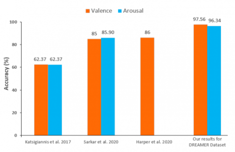
Lastly, Figure 12 demonstrates a summary of the comparison between the current study and the related state-of-the-art studies. We can see that the proposed method based on deep learning (DL) techniques outperforms in performance better than the latest studies based on DREAMER dataset.
Figure 12. The PETSFCNN-GSO-DNN network's results represented graphically
Table 4. Comparison of the performance of our proposed method with related state-of-the-art studies
|
Author |
Study |
Dataset |
Subjects |
Stimulus |
Classes |
Valence |
Arousal |
||
|
Acc % |
F1-s % |
Acc % |
F1-s % |
||||||
|
Subramanian et al. [21] |
NB |
ASCERTAIN |
58 |
Movie |
2 |
- |
60 |
- |
59 |
|
Wiem and Lachiri [22] |
SVM |
MAHNOB |
24 |
Video |
2 |
68.75 |
- |
64.23 |
- |
|
Hsu et al. [23] |
LS-SVM |
Private |
61 |
Music |
2 |
82.78 |
- |
72.91 |
- |
|
Katsigiannis and Ramzan [24] |
SVM+RBF Kernel |
DREAMER |
23 |
Audio-Visual |
2 |
62.37 |
53.05 |
62.37 |
57.98 |
|
Baghizadeh et al. [25] |
SVM-Polynomial SVM-Linear |
MAHNOB |
24 |
Video |
2 |
78.07 |
- |
82.17 |
- |
|
Santamaria-Granados et al. [26] |
DCNN |
AMIGOS |
40 |
Video |
2 |
75.00 |
- |
76.00 |
- |
|
Sarkar and Etemad [27] |
Self-Supervised (CNN) |
DREAMER |
23 |
Audio-Visual |
2 |
85.00 |
84.50 |
85.90 |
85.90 |
|
Harper and Southern [28] |
Bayesian-(CNN-LSTM) |
DREAMER |
23 |
Audio-Visual |
2 |
86.00 |
83.00 |
- |
- |
|
Our method |
PETSFCNN-GSO-DNN |
DREAMER |
23 |
Audio-Visual |
2 |
97.56 |
97.30 |
96.34 |
94.74 |
|
Private Data |
21 |
IAPS-Images |
2 |
76.19 |
75.65 |
80.95 |
79.89 |
||
Despite several different methods are proposed to detect and classify emotional states with high accuracy, but the need still exists for more efficient systems to improve the performance of classification. Moreover, In the field of affective computing, most of the experiments are suffering from a lack of datasets for training and testing their systems, data collecting (e.g., emotion triggering/evoking) is as yet a defy problem in this field. And for the aforementioned reasons, we introduced a novel PETSFCNN-GSO-DNN model for detecting and classifying affective states. The proposed method was implemented on two different datasets, where the first dataset was collected from 21 participants, while the second was a public DREAMER dataset that was collected from 23 subjects. The PETSFCNN-GSO-DNN model achieved a classification accuracy on the private dataset reach to 76.19% for valence and 80.95% for arousal respectively, whereas on the DREAMER dataset the PETSFCNN-GSO-DNN model achieved a classification accuracy reach to 97.56% for valence and 96.34% for arousal respectively. The empirical results have demonstrated that our proposed model outperforms and attains a better classification accuracy than state-of-the-art methods. To improve the accuracy and efficiency more, our future work will encompass using other deep learning techniques such as LSTM algorithms. Furthermore, we will use other physiological signals such as EEG to detect more affects.
[1] Tivatansakul, S., Ohkura, M. (2015). Emotion recognition using ECG signals with local pattern description methods. International Journal of Affective Engineering, 15(2): 51-61. https://doi.org/10.5057/ijae.ijae-d-15-00036
[2] Picard, R.W., Vyzas, E., Healey, J. (2001). Toward machine emotional intelligence: Analysis of affective physiological state. IEEE Transactions on Pattern Analysis and Machine Intelligence, 23(10): 1175-1191. https://doi.org/10.1109/34.954607
[3] Calvo, R.A., D'Mello, S. (2010). Affect detection: An interdisciplinary review of models, methods, and their applications. IEEE Transactions on Affective Computing, 1(1): 18-37. https://doi.org/10.1109/t-affc.2010.1
[4] Cao, W., Fang, Z., Hou, G., Han, M., Xu, X., Dong, J., Zheng, J. (2020). The psychological impact of the COVID-19 epidemic on college students in China. Psychiatry Research, 287: 112934. https://doi.org/10.1016/j.psychres.2020.112934
[5] Zhang, Y.D., Yang, Z.J., Lu, H.M., Zhou, X.X., Phillips, P., Liu, Q.M., Wang, S.H. (2016). Facial emotion recognition based on biorthogonal wavelet entropy, fuzzy support vector machine, and stratified cross validation. IEEE Access, 4: 8375-8385. https://doi.org/10.1109/access.2016.2628407
[6] El Ayadi, M., Kamel, M.S., Karray, F. (2011). Survey on speech emotion recognition: Features, classification schemes, and databases. Pattern Recognition, 44(3): 572-587. https://doi.org/10.1016/j.patcog.2010.09.020
[7] Mao, Q., Dong, M., Huang, Z., Zhan, Y. (2014). Learning salient features for speech emotion recognition using convolutional neural networks. IEEE Transactions on Multimedia, 16(8): 2203-2213. https://doi.org/10.1109/tmm.2014.2360798
[8] Yadollahi, A., Shahraki, A.G., Zaiane, O.R. (2017). Current state of text sentiment analysis from opinion to emotion mining. ACM Computing Surveys (CSUR), 50(2): 1-33. https://doi.org/10.1145/3057270
[9] Shu, L., Xie, J., Yang, M., et al. (2018). A review of emotion recognition using physiological signals. Sensors, 18(7): 2074. https://doi.org/10.3390/s18072074
[10] Cannon, W.B. (1927). The James-Lange theory of emotions: A critical examination and an alternative theory. The American Journal of Psychology, 39(1/4): 106-124. https://doi.org/10.2307/1415404
[11] Baig, M.Z., Kavakli, M. (2019). A survey on psycho-physiological analysis & measurement methods in multimodal systems. Multimodal Technologies and Interaction, 3(2): 37. https://doi.org/10.3390/mti3020037
[12] Kim, J. (2007). Bimodal emotion recognition using speech and physiological changes. Robust Speech Recognition and Understanding, 265: 280. https://doi.org/10.5772/4754
[13] Peter, C., Ebert, E., Beikirch, H. (2009). Physiological sensing for affective computing. In Affective Information Processing, pp. 293-310. https://doi.org/10.1007/978-1-84800-306-4_16
[14] Goshvarpour, A., Abbasi, A., Goshvarpour, A. (2017). An accurate emotion recognition system using ECG and GSR signals and matching pursuit method. Biomedical Journal, 40(6): 355-368. https://doi.org/10.1016/j.bj.2017.11.001
[15] Alshabeeb, I.A., Ali, N.G., Naser, S.A., Shakir, W.M. (2020). A clustering algorithm application in Parkinson disease based on k-means method. Computer Science, 15(4): 1005-1014.
[16] Liu, W., Qiu, J.L., Zheng, W.L., Lu, B.L. (2019). Multimodal emotion recognition using deep canonical correlation analysis. arXiv preprint arXiv:1908.05349.
[17] Rattanyu, K., Mizukawa, M. (2011). Emotion recognition based on ECG signals for service robots in the intelligent space during daily life. Journal of Advanced Computational Intelligence and Intelligent Informatics, 15(5): 582-591. https://doi.org/10.20965/jaciii.2011.p0582
[18] Dinde, S., Paithane, A.N. (2004). Human Emotion Recognition using Electrocardiogram Signals. International Journal on Recent and Innovation Trends in Computing and Communication, 2(2): 194-197.
[19] Sepúlveda, A., Castillo, F., Palma, C., Rodriguez-Fernandez, M. (2021). Emotion recognition from ECG signals using wavelet scattering and machine learning. Applied Sciences, 11(11): 4945. https://doi.org/10.3390/app11114945
[20] Russell, J.A. (1980). A circumplex model of affect. Journal of Personality and Social Psychology, 39(6): 1161. https://psycnet.apa.org/doi/10.1037/h0077714
[21] Subramanian, R., Wache, J., Abadi, M.K., Vieriu, R.L., Winkler, S., Sebe, N. (2016). ASCERTAIN: Emotion and personality recognition using commercial sensors. IEEE Transactions on Affective Computing, 9(2): 147-160. https://doi.org/10.1109/taffc.2016.2625250
[22] Wiem, M.B.H., Lachiri, Z. (2017). Emotion classification in arousal valence model using MAHNOB-HCI database. International Journal of Advanced Computer Science and Applications, 8(3): 318-323.
[23] Hsu, Y.L., Wang, J.S., Chiang, W.C., Hung, C.H. (2017). Automatic ECG-based emotion recognition in music listening. IEEE Transactions on Affective Computing, 11(1): 85-99. https://doi.org/10.1109/TAFFC.2017.2781732
[24] Katsigiannis, S., Ramzan, N. (2017). DREAMER: A database for emotion recognition through EEG and ECG signals from wireless low-cost off-the-shelf devices. IEEE Journal of Biomedical and Health Informatics, 22(1): 98-107. https://doi.org/10.1109/jbhi.2017.2688239
[25] Baghizadeh, M., Maghooli, K., Farokhi, F., Dabanloo, N.J. (2020). A new emotion detection algorithm using extracted features of the different time-series generated from ST intervals Poincaré map. Biomedical Signal Processing and Control, 59: 101902. https://doi.org/10.1016/j.bspc.2020.101902
[26] Santamaria-Granados, L., Munoz-Organero, M., Ramirez-Gonzalez, G., Abdulhay, E., Arunkumar, N.J.I.A. (2018). Using deep convolutional neural network for emotion detection on a physiological signals dataset (AMIGOS). IEEE Access, 7: 57-67. https://doi.org/10.1109/access.2018.2883213
[27] Sarkar, P., Etemad, A. (2020). Self-supervised ECG representation learning for emotion recognition. IEEE Transactions on Affective Computing. https://doi.org/10.1109/taffc.2020.3014842
[28] Harper, R., Southern, J. (2020). A Bayesian deep learning framework for end-to-end prediction of emotion from heartbeat. IEEE Transactions on Affective Computing. https://doi.org/10.1109/TAFFC.2020.2981610
[29] Burns, A., Greene, B.R., McGrath, M.J., et al. (2010). SHIMMER™–A wireless sensor platform for noninvasive biomedical research. IEEE Sensors Journal, 10(9): 1527-1534. https://doi.org/10.1109/jsen.2010.2045498
[30] Cuomo, S., De Pietro, G., Farina, R., Galletti, A., Sannino, G. (2016). A revised scheme for real time ECG signal denoising based on recursive filtering. Biomedical Signal Processing and Control, 27: 134-144. https://doi.org/10.1016/j.bspc.2016.02.007
[31] Berkaya, S.K., Uysal, A.K., Gunal, E.S., Ergin, S., Gunal, S., Gulmezoglu, M.B. (2018). A survey on ECG analysis. Biomedical Signal Processing and Control, 43: 216-235. https://doi.org/10.1016/j.bspc.2018.03.003
[32] Kiranyaz, S., Avci, O., Abdeljaber, O., Ince, T., Gabbouj, M., Inman, D.J. (2021). 1D convolutional neural networks and applications: A survey. Mechanical Systems and Signal Processing, 151: 107398. https://doi.org/10.1016/j.ymssp.2020.107398
[33] LeCun, Y., Bottou, L., Bengio, Y., Haffner, P. (1998). Gradient-based learning applied to document recognition. Proceedings of the IEEE, 86(11): 2278-2324. https://doi.org/10.1109/5.726791
[34] Schmidhuber, J. (2015). Deep learning in neural networks: An overview. Neural Networks, 61: 85-117. https://doi.org/10.1016/j.neunet.2014.09.003
[35] Murat, F., Yildirim, O., Talo, M., Baloglu, U.B., Demir, Y., Acharya, U.R. (2020). Application of deep learning techniques for heartbeats detection using ECG signals-analysis and review. Computers in Biology and Medicine, 120: 103726. https://doi.org/10.1016/j.compbiomed.2020.103726
[36] Islam, M.R., Islam, M.M., Rahman, M.M., et al. (2021). EEG channel correlation based model for emotion recognition. Computers in Biology and Medicine, 136: 104757. https://doi.org/10.1016/j.compbiomed.2021.104757
[37] Topic, A., Russo, M. (2021). Emotion recognition based on EEG feature maps through deep learning network. Engineering Science and Technology, an International Journal, 24(6): 1442-1454. https://doi.org/10.1016/j.jestch.2021.03.012
[38] Maheshwari, D., Ghosh, S.K., Tripathy, R.K., Sharma, M., Acharya, U.R. (2021). Automated accurate emotion recognition system using rhythm-specific deep convolutional neural network technique with multi-channel EEG signals. Computers in Biology and Medicine, 134: 104428. https://doi.org/10.1016/j.compbiomed.2021.104428
[39] Khare, S.K., Bajaj, V. (2020). Time–frequency representation and convolutional neural network-based emotion recognition. IEEE Transactions on Neural Networks and Learning Systems, 32(7): 2901-2909. https://doi.org/10.1109/TNNLS.2020.3008938
[40] Patterson, J., Gibson, A. (2017). Deep Learning: A Practitioner's Approach. O'Reilly Media, Inc.
[41] Srivastava, N., Hinton, G., Krizhevsky, A., Sutskever, I., Salakhutdinov, R. (2014). Dropout: A simple way to prevent neural networks from overfitting. The Journal of Machine Learning Research, 15(1): 1929-1958.