Menaka Radhakrishnan* | Karthik Ramamurthy | Avantika Kothandaraman | Gauri Madaan | Harini Machavaram
© 2021 IIETA. This article is published by IIETA and is licensed under the CC BY 4.0 license (http://creativecommons.org/licenses/by/4.0/).
OPEN ACCESS
To record all electrical activity of the human brain, an electroencephalogram (EEG) test using electrodes attached to the scalp is conducted. Analysis of EEG signals plays an important role in the diagnosis and treatment of brain diseases in the biomedical field. One of the brain diseases found in early ages include autism. Autistic behaviours are hard to distinguish, varying from mild impairments, to intensive interruption in daily life. The non-linear EEG signals arising from various lobes of the brain have been studied with the help of a robust technique called Detrended Fluctuation Analysis (DFA). Here, we study the EEG signals of Typically Developing (TD) and children with Autism Spectrum Disorder (ASD) using DFA. The Hurst exponents, which are the outputs of DFA, are used to find out the strength of self-similarity in the signals. Our analysis works towards analysing if DFA can be a helpful analysis for the early detection of ASD.
detrended fluctuation analysis, hurst parameter, self-similarity, typically developing, autism spectrum disorder
Autism Spectrum Disorder (ASD) is defined by a heterogeneous constellation of behavioural symptoms that appear over the initial growth stages of an individual. It is a type of neurodevelopmental disorder. ASD has changed from being a narrowly defined area to a highly researched field. Since its original delineation, the description of the core features of ASD as being social communication deficits and repetitive and unusual sensory–motor behaviours has not changed substantially. In a recent study, the Center for Disease Control (CDC), USA, estimates that the prevalence of ASD in the United States is 1 in 68, a significant increase in the past decade [1]. As research on ASD progresses at a rapid pace, ethology and development studies appear to be very different, leading to the perception of ASD in a variety of cognitive, behavioural and neural pathways and subtypes. The power of the EEG used as a function of brain analysis continues to evolve as new methods of analysing and extracting information from biophysical signals are developed. Methods of analysing complex time series generated by complex networks, such as the human brain, may allow for network variability to be viewed from time series estimates. Based on this, a set of non-linear or 'invariant measures’ from EEG signals must reflect the neural potential in the brain that produces the signals [2]. Ionic current flows in the signals causes voltage fluctuations as measured by EEG within the neurons of the brain and then run into algorithms of classification based on band frequency [3, 4], custom signal thresholds [5], alpha band frequency (SVM, ML algorithms) [6] and Higuchi Fractal Dimension [7]. These procedures give normal or abnormal EEG activity that might not be normally seen [8]. These procedures record in-brain activity in patients suffering from Cerebral Palsy (CP), Parkinson and schizophrenia and autism [9]. Diagnostic applications generally focus on the spectral content of EEG, that is, the type of neural oscillations that can be observed in EEG signals. In recent years, a number of non-linear analytical methods, including DFA, have been developed as an important tool for obtaining long-range (auto-)correlations in time series and have become the most widely used method for determining (mono-) fractal scaling properties and long-distance noisy, nonstationary time series [10]. Earlier studies using DFA talk about investigating heart signals [11], where the autocorrelation of non-stationary Electrocardiogram (ECG) signals was analysed. Arsac and Deschodt-Arsac [12] exploited DFA to evaluate the multifractality displayed in electroencephalogram (EEG) signals obtained from subjects with sleep apnea. Nonlinear primitive features can effectively analyse brain dynamics in the EEG signal produced. Recent research shows that applications of fractal-based techniques are effective to estimate the degree of nonlinearity in a signal. Autism at early ages has been a tough complexity in the field, as trials have proved to be at most random in coherence to short term or long term anomaly. With regressive results, implications of imitation, motor, and play deficits for communication-based intervention are tested and prevented to some degree [13]. Without a definite distinction, given the few randomized and controlled treatment trials that have been carried out, the existing models that have been tested, and with the large differences in interventions being published, using DFA we intend to provide an undemanding analysis of Autism Spectrum Disorder [14].
The process followed for the entire research is shown in Figure 1.
Figure 1. The workflow process followed
2.1 EEG data collection
The first step in processing any kind of signal is to collect initial raw data. Metadata includes the sampling interval, the position of the EEG electrodes, the number of electrodes, the total number of sample points, etcetera. The signals were sampled at 500 Hz (hertz). EEG values are always taken as a relative measure, and this is known as EEG montage. Different montages include bipolar, Laplacian, common electrode reference, average and weighted averaged references [15]. For this research, the EEG data were collected with average reference electrodes. The research participants were aged 3-7 years. Equal number of datasets were acquired from both TD and children diagnosed with ASD.
Around 13,000 sample points were recorded for each EEG channel in each dataset. A total of 10,000 EEG signal samples were selected for each child across 19 different EEG channels. The sample points picked were the first 10,000 sample points of the EEG signals for all children. Since each child had a different number of sample points recorded, that ranged from 10,000 to 15,000, the first 10,000 sample points were chosen for all to ensure uniformity in the number of sample points. The research participants were all engaged in some visually stimulating activity.
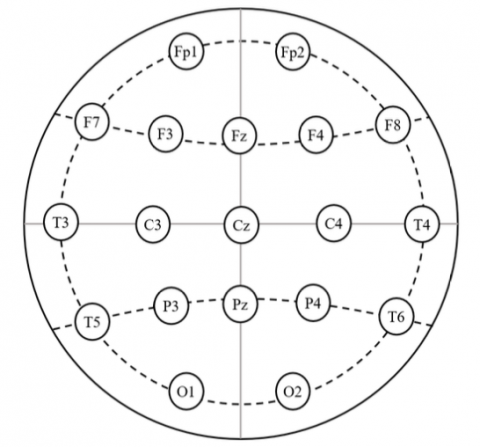
The International 10-20 system of electrode placement positions was adopted. Figure 2 shows the pictorial representation of the electrode placement. The positions were Fp1, Fp2, F7, F3, Fz, F4, F8, P3, P4, Pz, T3, T5, T4, T6, O1, O2, C3, C4 and Cz [16] as shown in Figure 2.
Figure 2. International 10-20 system of EEG electrode placement
2.2 Preprocessing the acquired EEG signals
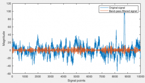
Data preprocessing is the first and foremost step in signal data analysis. EEG data in particular contain a lot of noise and inconsistencies. Noise in EEG data exists due to both external/environmental conditions, as well as internal/physiological conditions [17]. Several methods exist to remove such existing noise from the data. Here, bandpass [18] and Gaussian filters were chosen as noise removal techniques. The parameters for the bandpass filter were chosen in such a way that only frequencies between 8 and 12 Hz were allowed to pass through, the sampling rate being 500 Hz. The Gaussian filter used here is a narrow-band filter that calculates the Gaussian noise in the frequency domain and removes it. This filter was specifically designed for this analysis. The inputs of the filter are the signal data, the sampling rate of the signals, peak frequency (10 Hz: since alpha band ranges from 8-12 Hz) and a standard deviation of 2 Hz (10 ± 2 Hz). The bandpass filtered signal is depicted in Figure 3.
Figure 3. Original (blue) and bandpass filtered signals (orange) superimposed for comparison
Since the focus of the analysis is on the alpha band as in Table 1, band pass filters were used to allow only the required band of frequencies to pass through for analysis [19] (Figure 3). The alpha band comprises the range of EEG signal frequencies from 8-12 Hz. This is the most prominent and easy-to-observe band of frequencies during wakefulness and mental concentration. At the time of recording the EEG signals, the subjects were engaged in some visually stimulating activities that required their mental attention and thinking and a sense of relaxed awareness. Beta waves are normally found in adults at the time of heightened mental concentration. Gamma waves are also found to be most prominent during heightened emotions such as fear or anxiety.
Table 1. The ranges for different frequency bands of EEG signals
|
FREQUENCY (HZ) |
BAND |
|
0-3 |
Delta |
|
4-7 |
Theta |
|
8-12 |
Alpha |
|
13-30 |
Beta |
|
30-100 |
Gamma |
2.3 Feature extraction by detrended fluctuation analysis
DFA is used to determine the self-affinity of a signal [20]. Self-affinity is a property of fractal type time-series data [20, 21]. It describes the way in which a small segment of the signal represents the whole signal structure. The output of DFA is the Hurst Parameter (a dimensionless parameter), which describes the ‘long-term memory’ of the signal, i.e., it determines if the series is more/less/equally likely to increase if it has increased in the previous steps. If the Hurst exponent is close to 0.5, it indicates that the series progresses as a random noise structure. Hurst values closer to 1 indicate strong positive auto-correlation [22].
It is recommended to perform the analysis on the power-spectrum or on the amplitude spectrum of the signal rather than on the original time-series signal. To do that, wavelet convolution is performed on the signal to convert it into amplitude time-series shown in Figure 4 and then DFA is performed on the signal [23].
Figure 4. Analysis of the EEG signals
In Figure 4, the blue graph represents the bandpass filtered EEG signal, whereas the orange graph lines correspond to the amplitude time-series signal.
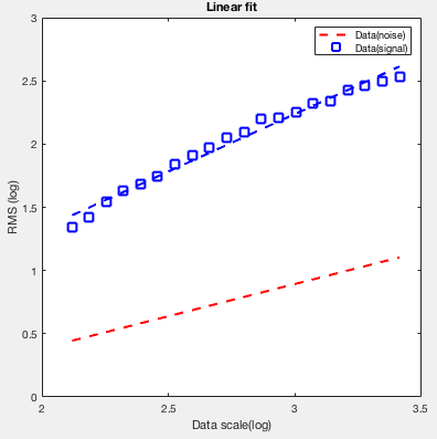
Steps to perform DFA are (1) Convert the signal into a mean-centered cumulative sum of values (Eq. (1)) (Figure 5), (2) Define log-spaced scales, (3) Choose a scale, split the signal into epochs based on the chosen scale, detrend it and compute its individual Root Mean Square (RMS) values (Eq. (2)), (4) Repeat step 3 for all the other scales, and find the overall average of each scale’s RMS, (5) Compute a linear fit between the log-scales and the RMS values [22]. The slope of the obtained linear fit gives the Hurst parameter depicted in Figure 6.
Given a bounded time-series xt of length N, the mean-centered cumulative sum would be given as,
$X_{t}=\sum_{i=1}^{t}\left(x_{i}-\langle x\rangle\right)$ (1)
where, Xt is an unbounded mean-centered cumulative sum of the series and <x> is the mean of the series. xi represents each point in the signal.
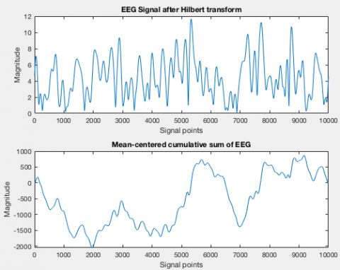
In the second picture of Figure 5, both the axes show a set of values in the negative range and a sharp increase of magnitude in signal amplitude. This is a plot of the mean-centered cumulative sum of values. This helps us identify the mean of the sample points in relation to the sample points (10,000 sample points) of the process at that time. Some of the initial sample points of the EEG signal tend to be lesser than the overall mean, giving rise to negative ordinates. When the cumulative sum is calculated, the amplitude tends to increase/decrease based on the previous calculated values. This erratic behavior is to be expected at this stage and hence is reflected on the ordinates of the plot.
Figure 5. Mean-centered cumulative sum output of the input EEG
The RMS deviation from the trend is given by,
$F(n)=\sqrt{\frac{1}{N} \sum_{t=1}^{N}\left(X_{t}-Y_{t}\right)^{2}}$ (2)
where, Yt is the resulting piecewise sequence of straight-line fits, X. A linear fit is determined using the obtained RMS values.
Figure 6. Sample of the linear fit of the log scales and the log RMS for both the signal and a random noise input
In Figure 6, slope of the linear fit of the signal gives the value of the Hurst parameter, and here, the observed fit (blue) is for the Fz electrode of a TD child, H=0.9069. The signal was first converted into a zero-mean Gaussian, upon which Hilbert transform was performed. Based on the sampling rate, the signal was converted into frequency domain using Fourier transform and the frequency was normalised. Using the peak frequency as 10 Hz and a standard deviation of ± 2 Hz, Gaussian functions were used for conversion, upon which Hilbert transform functions were applied. The output of this step gives us an amplitude time-series, similar to that of Morlet Wavelet Convolution. 20 log scales were chosen and the log range was taken from 1% of the signal to 20% of the signal.
The above steps were performed on all the processed 19 channels to analyse the Hurst Parameter individually.
Significance testing: For analysis of our obtained results, significance analysis was done in addition to the basic statistical parameters such as mean and standard deviation. The threshold for the p-statistic was taken as 0.1, and values above 0.1 were deemed statistically insignificant for analysis and were rejected. Significance analysis was done on all the channels for both TD children and children with ASD.
Analysis was carried out at the alpha band (8 - 12 Hz) shown in Table 1 of frequencies. 10 Hz was chosen for the purpose of analysis.
Analysing the overall mean of an entire brain region may produce tangible results, but may not be fully accurate to ascertain the working of the brain. Each channel must be analysed individually to compare and contrast the effects of long-term time-series memory. For TD children, there were 5 particular channels that had the least standard deviation across different children. This implies that the values of the Hurst parameter followed a certain consistency in these particular channels for TD children. The 5 channels that had the least standard deviation and high similarity for different TD children were found to be F3, P4, T5, C3 and O1. Similarly, for children with ASD, there were 3 particular channels that had the least standard deviation across different children. This implies that the values of the Hurst parameter followed a certain consistency in these particular channels for children with ASD. The 3 channels that had the least standard deviation and high similarity for different children with ASD were found to be Fp1, Fp2 and O2.
Figure 7. (Left) TD children. (Right) Children with ASD. Electrodes showing least standard deviation
It can be seen from Figure 7 that 4 out of 5 regions are on the left side of the brain, indicating that TD children of 3-7 years of age typically showed similar strengths of self-affinity on the left side of the brain. Similarly, for children with ASD, it can be seen that 2 out of 3 regions are on the frontal part of the brain. This observation could help us differentiate between TD children and children with ASD with respect to the regions of the brain that show similarity/dissimilarity. Based on the results, it was observed that the Hurst values on the left side of the brain for TD children showed some similarity when compared to children with ASD that showed the same on the frontal region. This observation could be a possible differentiating factor.
Figure 8. The channels that showed the least standard deviation in both TD children and children with ASD (the green cones on the plots represent the mean)
The channels in Figure 8 showed the least deviation from the mean across different children, and can be used as a comparative measure. The expected mean and standard deviation are tabulated in Table 2.
Table 2. Depicting the channels in both TD children and children with ASD with the least standard deviation. (STD DEV = Standard deviation)
|
STATE |
CHANNEL |
MEAN ± STD DEV |
P-VALUE |
|
TD |
F3 |
0.98 ± 0.04 |
0.28 |
|
P4 |
1.10 ± 0.05 |
0.05 |
|
|
T5 |
0.99 ± 0.04 |
0.56 |
|
|
C3 |
1.15 ± 0.04 |
0.08 |
|
|
O1 |
0.98 ± 0.04 |
0.23 |
|
|
ASD |
Fp1 |
1.12 ± 0.05 |
0.6 |
|
Fp2 |
1.1 ± 0.04 |
0.6 |
|
|
O2 |
1.00 ± 0.04 |
0.26 |
The p-statistic was calculated for Hurst values for each channel and for all TD children and children with ASD. The threshold value was chosen as 0.1. Only for p-values below the threshold, the values were deemed statistically significant, and the null hypothesis was rejected. Otherwise, the null hypothesis was accepted.
Normally, the p-statistic is chosen as 0.05. During analysis, it was found that only two channels showed a p-statistic below 0.05. Since these two channels showed highly fluctuating Hurst values with a high standard deviation, they are not appropriate for distinguishing between TD children and children with ASD. As a result, for this application, the p-value threshold was increased to 0.1 instead. When this was done, the C3 channel with p-value 0.08 produced better results while differentiating between the two (TD children and children with ASD).
Figure 9. Plot depicting the p-value for all the channels. Red line marks the 0.1 threshold
Table 3. The p-values of the 5 channels with p < 0.1
|
CHANNEL |
P-VALUE |
|
P3 |
0.002 |
|
P4 |
0.052 |
|
Pz |
0.066 |
|
T6 |
0.018 |
|
C3 |
0.083 |
It can be observed from Figure 9 that the p-statistic attains a value < 0.1 only in 5 channels, P3, P4, Pz, T6 and C3, indicating that these channels hold a statistically significant difference between the TD children and children with ASD, in terms of the Hurst parameter. The corresponding values can be seen in Table 3 (The p-values for these channels lie below the marked threshold of 0.1). Some of the other 4 channels show a p-value lesser than 0.08 and theoretically and statistically, those could have been better choices for differentiation. However, it was the C3 channel (owing to a much lower standard deviation), that showed a better accuracy while classification.
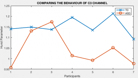
Amongst all the 5 channels with p-values below 0.1, the C3 channel with p = 0.08, showed a 71% accuracy while differentiating between TD children and children with ASD.
Figure 10. The C3 channel (p=0.08) showed the highest accuracy while differentiating, amongst all other channels that had p-statistic values < 0.1
In Figure 10, only 2 out of 7 participants had Hurst values which fell in the range of TD children’s Hurst values. It should also be noted that the C3 channel is one of the 5 channels that showed the least standard deviation in TD children.
Higher the value of the Hurst exponent, stronger the positive auto-correlation. After the analysis of both TD children and children with ASD, it was found that no channel showed a Hurst value less than or equal to 0.5. This means that the signals were not random walk signals or anti-persistent time-series signals in nature.
While the Hurst exponent can tell us about the strength of positive auto-correlation of a signal very well, it is quite specific to the signal being analysed and the activity being performed by the individuals. Finding a common ground of similarities/dissimilarities between different groups is quite challenging, but not impossible nonetheless. This also makes the process of classification harder.
There were a few limitations/constraints that were experienced while this research was carried out. One such limitation was that the values obtained are highly specific to the datasets acquired. The analysis was not carried out for EEG signals with different metadata, so it is challenging to generalise this approach. The datasets were acquired from less than 20 subjects making the results more prone to bias and less accuracy. Due to ethical and legal restrictions, it is quite difficult to obtain data pertaining to individuals with ASD. The discussed nonlinear algorithm has not been applied to a variety of subjects at a large scale in the real-world, so its effect on a large number of subjects has not yet been determined. Although there are numerous models for classification of ASD, there is no specific standard to compare results with. This is because ASD is a broad spectrum disorder that encompasses different types of neurodevelopmental issues over a large scale.
All the participants in the study were exposed to the same audio and visual stimulus. This could be inferred as a possible reason as to why there were no drastic differences in the Hurst values of the two types of individuals.
Possible future directions could be the acquisition of EEG data from a variety of different subjects on a larger scale, with varying metadata for added diversity, the devising of a reasonably accurate classification model to deal with the randomness, real-world deployment of the models to assess its accuracy and some optimisation techniques to further improve results.
This research was funded by the Department of Science and Technology DST under Science for Equity, Empowerment, and Development (SEED) Division (File No: SEED/TIDE/092/2016). We would like to render our sincere thanks to the Sri Ramachandra Institute of Higher Education and Research for their kind support and assistance in data acquisition.
[1] Kanner, L. (1943). Autistic disturbances of affective contact. Nervous Child, 2(3): 217-250.
[2] Irimiciuc, S.A., Zala, A., Dimitriu, D., Himiniuc, L.M., Agop, M., Toma, B.F., Eva, L. (2021). Novel approach for EEG signal analysis in a multifractal paradigm of motions. Epileptic and Eclamptic Seizures as Scale Transitions. Symmetry, 13(6): 1024. https://doi.org/10.3390/sym13061024
[3] Al-Galal, S.A., Alshaikhli, I.F.T. (2017). Analyzing brainwaves while listening to Quranic recitation compared with listening to music based on EEG signals. International Journal on Perceptive and Cognitive Computing, 3(1).
[4] Bastos, N.S., Marques, B.P., Adamatti, D.F., Billa, C.Z. (2020). Analyzing EEG signals using decision trees: A study of modulation of amplitude. Computational Intelligence and Neuroscience. https://doi.org/10.1155/2020/3598416
[5] Chuang, J., Nguyen, H., Wang, C., Johnson, B. (2013). I think, therefore I am: Usability and security of authentication using brainwaves. In International Conference on Financial Cryptography and Data Security, pp. 1-16. https://doi.org/10.1007/978-3-642-41320-9_1
[6] Ahmadi, N., Pei, Y., Pechenizkiy, M. (2017). Detection of alcoholism based on EEG signals and functional brain network features extraction. In 2017 IEEE 30th International Symposium on Computer-Based Medical Systems (CBMS), pp. 179-184. https://doi.org/10.1109/CBMS.2017.46
[7] Radhakrishnan, M., Won, D., Manoharan, T.A., Venkatachalam, V., Chavan, R.M., Nalla, H.D. (2021). Investigating electroencephalography signals of autism spectrum disorder (ASD) using Higuchi Fractal Dimension. Biomedical Engineering/Biomedizinische Technik, 66(1): 59-70. https://doi.org/10.1515/bmt-2019-0313
[8] Pernet, D.C. (2019). Electroencephalography (EEG). The University of Edinburgh. https://www.ed.ac.uk/clinical-sciences/edinburgh-imaging/research/themes-and-topics/medical-physics/imaging-techniques/electroencephalography, accessed on 8 August 2021.
[9] Abd Rahman, F., Othman, M.F., Shaharuddin, N.A. (2015). Analysis methods of EEG signals: a review in EEG application for brain disorder. Jurnal Teknologi, 72(2). https://doi.org/10.11113/jt.v72.3886
[10] Kantelhardt, J.W., Koscielny-Bunde, E., Rego, H.H., Havlin, S., Bunde, A. (2001). Detecting long-range correlations with detrended fluctuation analysis. Physica A: Statistical Mechanics and its Applications, 295(3-4): 441-454. https://doi.org/10.1016/S0378-4371(01)00144-3
[11] Pranata, A.A., Adhane, G.W., Kim, D.S. (2017). Detrended fluctuation analysis on ECG device for home environment. In 2017 14th IEEE Annual Consumer Communications & Networking Conference (CCNC), pp. 126-130. https://doi.org/10.1109/CCNC.2017.7983093
[12] Arsac, L.M., Deschodt-Arsac, V. (2018). Detrended fluctuation analysis in a simple spreadsheet as a tool for teaching fractal physiology. Advances in Physiology Education, 42(3): 493-499. https://doi.org/10.1152/advan.00181.2017
[13] Landa, R. (2007). Early communication development and intervention for children with autism. Mental Retardation and Developmental Disabilities Research Reviews, 13(1): 16-25. https://doi.org/10.1002/mrdd.20134
[14] Rogers, S.J., Vismara, L.A. (2008). Evidence-based comprehensive treatments for early autism. Journal of Clinical Child & Adolescent Psychology, 37(1): 8-38. https://doi.org/10.1080/15374410701817808
[15] Britton, J.W., Frey, L.C., Hopp, J.L. (2016). Electroencephalography (EEG): An Introductory Text and Atlas of Normal and Abnormal Findings in Adults, Children, and Infants. NCBI, https://www.ncbi.nlm.nih.gov/books/NBK390353/, accessed on 8 August 2021.
[16] Rojas, G.M., Alvarez, C., Montoya, C.E., de la Iglesia-Vayá, M., Cisternas, J.E., Gálvez, M. (2018). Study of resting-state functional connectivity networks using EEG electrodes position as seed. Frontiers in Neuroscience, 12: 235. https://doi.org/10.3389/fnins.2018.00235
[17] Jadav, G.M., Lerga, J., Štajduhar, I. (2020). Adaptive filtering and analysis of EEG signals in the time-frequency domain based on the local entropy. EURASIP Journal on Advances in Signal Processing, 2020(1): 1-18. https://doi.org/10.1186/s13634-020-00667-6
[18] Brihadiswaran, G., Haputhanthri, D., Gunathilaka, S., Meedeniya, D., Jayarathna, S. (2019). EEG-based processing and classification methodologies for autism spectrum disorder: A review. Journal of Computer Science, 15(8). https://doi.org/10.3844/jcssp.2019.1161.1183
[19] Bosl, W.J., Tager-Flusberg, H., Nelson, C.A. (2018). EEG analytics for early detection of autism spectrum disorder: A data-driven approach. Scientific Reports, 8(1): 1-20. https://doi.org/10.1038/s41598-018-24318-x
[20] Alçіn, Ö.F., Siuly, S., Bajaj, V., Guo, Y., Şengu, A., Zhang, Y. (2016). Multi-category EEG signal classification developing time-frequency texture features based Fisher Vector encoding method. Neurocomputing, 218: 251-258. https://doi.org/10.1016/j.neucom.2016.08.050
[21] Likens, A.D., Nick, S. (2020). A tutorial on fractal analysis of human movements. Biomechanics and Gait Analysis, 313-344. https://doi.org/10.1016/B978-0-12-813372-9.00010-5
[22] Márton, L.F., Brassai, S.T., Bakó, L., Losonczi, L. (2014). Detrended fluctuation analysis of EEG signals. Procedia Technology, 12: 125-132. https://doi.org/10.1016/j.protcy.2013.12.465
[23] Cohen, M.X. (2019). Data Analysis Lecturelets. http://mikexcohen.com/lectures.html, accessed on 8 August 2021.