Mahima Lakra* | Sanjeev Kumar
© 2021 IIETA. This article is published by IIETA and is licensed under the CC BY 4.0 license (http://creativecommons.org/licenses/by/4.0/).
OPEN ACCESS
This paper proposes a variational approach by minimizing the energy functional to compute the disparity from a given pair of consecutive images. The partial differential equation (PDE) is modeled from the energy function to address the minimization problem. We incorporate a distance regularization term in the PDE model to preserve the boundaries' discontinuities. The proposed PDE is numerically solved by a cellular neural network (CeNN) algorithm. This CeNN based scheme is stable and consistent. The effectiveness of the proposed algorithm is shown by a detailed experimental study along with its superiority over some of the existing algorithms.
belief propagation, cellular neural network, distance regularization term, energy minimization
Stereo matching has a profound impact on computer vision tasks. It is commonly used to compute 3D depth information from stereo images in the disparity map context. For depth information, 2D stereo images are projected as coordinates in 3D by searching for correspondence pairs between these stereo images. Disparity refers to the distinction in an object's image region, which is visible through the left and right eyes. Disparity gives a method to determine the spatial connection between points and surfaces in a scene without any significant information level. If new objects enter the scene, then the observed disparity would be a term for making precise decisions using knowledge of objects' location and velocity in 3D space. There are numerous approaches to estimate the disparity; feature-based [1-4], area-based based [5-7], phase-based based [8-11] and energy-based based [12-20]. These algorithms establish a relationship among few selected features that have been extracted from the images [1, 2], curves based [3, 21, 22], line segments based [12, 23], and including area pixels based [24, 25]. Despite their enormous success, these studies fail to yield complete information on the field of interest.
The first step of feature-based methods is to detect disparity for specific ground control points, and this elegance of techniques was widely used. Special filters and edge-based techniques are used to calculate ground control points. A significant advantage of the feature-based methods is to obtain accurate results and control the appropriate amount of effects. Therefore, it increases the computation time for the whole process. Further, these approaches do not provide a dense depth map required in many applications.
In phase-based methods, the disparity with sub-pixel accuracy was achieved without subpixel feature detection and localization. The authors [26] show the stability of the bandpass phase behavior and instabilities of the phase near singularities. The Fourier phase is another data technique class, which is considered a form of slope-based optical flow strategy. The derived time is approximated in the scheme by the contrast between the right and left Fourier phase images.
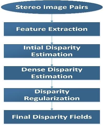
Energy minimization-based methods are associated with the solution of the correspondence problem in a regularization and minimization formulation [4, 12, 20, 27]. The authors [28] proposed a graph cut algorithm, and this approach solved the optimization problem in a better and efficient way. A region-dividing block matching algorithm was proposed by Kim et al. [29] to estimate dense disparity and computes within a shape-adaptive window. The variational approach [20] merges impressive and robust tools like regularization and multiscale to achieve depth directly while protecting depth discontinuities. Figure 1 shows the block diagram of the algorithm, and the dense disparity vectors are calculated from low to high-resolution fields using a region dividing technique and shape-adaptive matching windows [20].
Figure 1. Block diagram of energy minimization methods [20]
The disparity d between two consecutive pair images X1 and X2 are obtained by minimizing the energy functional from the open bounded set $\Omega \subseteq R^{2}$ as:
$\begin{aligned} E(d)=& \int_{\Omega}\left(X_{1}(r)-X_{2}(r+d)\right)^{2} d r+\\ & \alpha \int_{\Omega} \varphi\left(\nabla d, \nabla X_{1}\right) d r \end{aligned}$ (1)
where, $\alpha$ is a Lagrange multiplier and the potential function $\varphi\left(\nabla d, \nabla X_{1}\right)$ is defined as
$\nabla\left(\varphi\left(\nabla d, \nabla X_{1}\right)\right)=g\left(\left|\nabla X_{1}\right|^{2}\right) \nabla d$ (2)
The diffusivity function $g\left(\left|\nabla X_{1}\right|^{2}\right)$ is defined as
$g\left(\left|\nabla X_{1}\right|^{2}\right)=\frac{1}{\left(1+\left|\nabla X_{1}\right|^{2}\right)^{2}}$ (3)
The minimization problem written in the form of a parabolic system by using the Euler-Lagrange equation [20]
$$\frac{\partial d}{\partial t}=\alpha \operatorname{div}\left(g\left(\left|\nabla X_{1}\right|^{2}\right) \nabla d\right)+\left(X_{1}(r)-X_{2}(r+\right.
$$d)) $\frac{\partial X_{2}(r+d)}{\partial x}$ (4)
In Eq. (4), the diffusivity function g\left(\left|\nabla X_{1}\right|^{2}\right) plays the role of the discontinuity marker, and it remains smooth at the boundaries. The energy minimization formulation computes the disparity fields with reasonable accuracy, but it consists of a local minimum problem and includes computational load problems to solve PDEs. Occasionally, stereo images cannot be accurately adjusted to calculate disparity if cameras' arrangement can be marginally pivoted of the level. Regularization of vector fields, which includes both fidelity and smoothness, needs to be more appropriate, and so must the optimization technique of the system. Most of the methods face the object boundary problem and do not preserve the discontinuities at boundaries.
The paper's key feature is to build a model that maintains the edge discontinuity. A distance regularization term (DRT) is added to the model to create the edge discontinuity. DRT gives a significant advantage as it maintains the forward and backward diffusion. DRT satisfies the boundedness property, allowing us to keep the discontinuity between edges in the disparity map. An iterative technique is used to solve the parabolic partial differential equation (PDE). Several algorithms exist for computing disparity, but a data-driven CeNN scheme is proposed for a beneficial network type. The CeNN can be implemented easily with low computation costs. The CeNN architecture is obtained by discretizing the PDE using the central difference method. The modified PDE is demonstrated in the CeNN form and used to create the template matrices for the proposed CeNN system. The proposed scheme is capable of obtaining disparity without any parameter settings. The stability of the proposed method shows robustness against perturbations in the input images. Finally, in numerical experiments, RMSE and BMP matrices on some standard images are considered.
The remainder outline is organized as follows: Sect. 2 covers the formation of proposed PDE by minimizing the energy functional and discusses the discretization of proposed PDE into CeNN formation. This section ends with computing the CeNN template matrices. In Sect. 3, the convergence of the proposed system has been shown. The results and discussion present in Sect. 4, and the managerial implications of minimizing the energy functional to compute the disparity from a given pair of consecutive images has been added in section 5. Finally, the conclusions are drawn in Sect. 6.
The process to obtain the CeNN template matrices is described in this section. These template matrices are obtained using the spatial discretization over the modified PDE proposed in the study.
2.1 Derived partial differential equation
Consider the energy functional $\varepsilon(d)$ for the disparity function d is defined as
$\varepsilon(d)=\alpha D_{p}(d)+\varepsilon_{e x t}(d)$ (5)
The external energy function depends upon the data of interest, and it is defined so that it minimizes the $\varepsilon(d)$. The parameter $\alpha$ can take any constant positive value. The regularization function $D_{p}(d)$ is defined as
$D_{p}(d)=\int_{\Omega} p(|\nabla d|) d \Omega$ (6)
where, $p:[0, \infty) \rightarrow \mathbb{R}$ is the energy density function. The Gateaux derivative of the $D_{p}(d)$ functional is computed as
$\frac{\partial D_{p}(d)}{\partial t}=-\operatorname{div}\left(d_{p}(|\nabla d|) \nabla d\right)$ (7)
where, $\operatorname{div}(.)$ is the divergence operator and $\nabla$ defined as a gradient operator. Following Euclidean norm is used for the computation:
$|\nabla U|=\sqrt{\left(\frac{d U}{d x}\right)^{2}+\left(\frac{d U}{d y}\right)^{2}}$ (8)
The following equation described the DRT as [30];
$d_{p}(d)=\frac{p^{\prime}(s)}{s}$ (9)
A preferable function $p(\cdot)$ for the DRT taken as
$p(s)=\left\{\begin{array}{ll}\frac{1}{2 \pi^{2}}(1-\cos (2 \pi s)) & s \leq 1 \\ \frac{1}{2}(s-1)^{2} & s>1\end{array}\right\}$ (10)
The energy density function p(s) has two minimum points $s=0$ and $s=1$. It is twice differentiable in $[0,1)$, and the first-order derivative of a differentiable function $p(s), \quad s \in[0, \infty)$ is defined as
$p^{\prime}(s)=\left\{\begin{array}{ll}\frac{1}{2 \pi}(\sin (2 \pi s)) & s \leq 1 \\ (s-1) & s \geq 1\end{array}\right\}$ (11)
The function d satisfies the conditions, $\left|d_{p}(s)\right|<1$ , for all $S \in[0, \infty)$ and
$\lim _{s \rightarrow \infty} d_{p}(s)=\lim _{s \rightarrow 0} d_{p}(s)=1$.
This diffusion rate depends on the energy density function p(s) and assumes a positive or negative rate accordingly. The diffusion is forward diffusion when $d_{p}(|\nabla d|)$ is positive, and the diffusion is backward diffusion when $d_{p}(|\nabla d|)$ is negative. This diffusion is also known as forward-and-backward diffusion.
The energy functional $\varepsilon(d)$ in an image domain $\Omega \subseteq R^{2}$ is minimized to regularize the vector fields as follows
$\min _{d} \varepsilon(d)=\alpha D_{p}(d)+|\nabla d| A_{g}(d)+\lambda_{1} L_{g}(d)$ (12)
where, the constant parameter $\lambda_{1}>0$. The function $D_{p}(d)$ is defined as the same as Eq. (6). The energy sub functionals $A_{g}(d)$ and $L_{g}(d)$ for image sequence $X_{1}$ and $X_{2}$ are defined by
$A_{g}(d)=\int_{\Omega}|\nabla d(x, y)| d \Omega$ (13)
$L_{g}(d)=\int_{\Omega}\left(X_{1}(x, y)-X_{2}(x+d, y)\right) d \Omega$ (14)
After applying the Euler Lagrange method, the proposed energy minimization function is defined as
$\frac{\partial d}{\partial t}=\alpha \operatorname{div}\left(d_{p}\left(\left|\nabla X_{1}\right|\right) \nabla d\right)+|\nabla d| \operatorname{div}\left(\frac{\nabla d}{|\nabla d|}\right)$$+\lambda_{1}\left(X_{1}(x, y)-X_{2}(x+d, y)\right) \frac{\partial X_{2}(x+d, y)}{\partial x}$ (15)
with initial disparity $d(x, y, 0)=d_{0}(x, y)$ and Neumann-type boundary conditions. The first term on the right-hand side in Eq. (15) follows the DRT diffusion effect, while the second and third terms express energy. The DRT $d_{p}(\cdot)$ is defined in Eq. (9). The property of forward-and-backward diffusion works for (15) in three steps as follows
2.2 Initial disparity estimation
Let S be the set of pixels in the image, and L is the label set that is finite. A labeling assigns a label F to each pixel $F_{p} \in L$. The following energy minimizing function expresses the labeling quality:
$E(F)=\sum_{p \in P} C_{p}\left(F_{P}\right)+\sum_{(p, q \in N)} M\left(F_{p}-F_{q}\right)$ (16)
where, the four connected image grid graphs have N edges. The discontinuity cost $M\left(F_{p}, F_{q}\right)$ measures the cost between two neighboring pixels $F_{P}$ and $F_{q} \cdot C_{p}\left(F_{P}\right)$ refers to the data cost of detecting a label $F_{P}$ for pixel p. Let $n_{p \rightarrow q}^{t}$ be the message at iteration t (node p sends to a neighboring node q). The iterative scheme for message updation $F_{p} \in L$ is defined by minimizing as
$n_{p \rightarrow q}^{t}\left(F_{q}\right)=\min _{F_{p}}\left(\begin{array}{l}C_{p}\left(F_{P}\right)+M\left(F_{p}-F_{q}\right) \\ +\sum_{s \in N(p) \backslash q} n^{t-1}{ }_{p \rightarrow q}\left(F_{q}\right)\end{array}\right)$ (17)
where, $N(p) \backslash q$ expresses the neighbors of p not containing q. Choose label F that minimize the belief vector at time T for each node expressed as
$B_{q}\left(F_{q}\right)=C_{q}\left(F_{q}\right)+\sum_{p \in N(q)} n_{p \rightarrow q}^{T}\left(F_{q}\right)$ (18)
The initial disparity is solved by the iterative belief propagation Eq. (18). The belief propagation calculation works by passing messages around the graphs noted from four related image frameworks and all nodes being given in parallel [31].
2.3 Spatial discretization
To compute the CeNN templates matrices in a simple form, the parabolic Eq. (15) is discretized using finite difference methods and the central difference method. We can write Eq. (15) in modified form as follows
$\frac{\partial d(x, y)}{\partial t}=\alpha \nabla^{T}\left(d_{p}\left(\left|\nabla X_{1}(x, y)\right|\right) \nabla d(x, y)\right)$
$+\lambda_{1}\left(X_{1}(x, y)-X_{2}(x+d, y)\right) \frac{\partial X_{2}(x+d, y)}{\partial x}$
$+|\nabla d| \nabla^{T}\left(\frac{\nabla d(x, y)}{|\nabla d|}\right)$ (19)
After simplifying the above PDE, the simple way is defined as
$\frac{\partial d(x, y)}{\partial t}=\alpha \frac{\partial}{\partial x}\left(d_{p}\left(\left|\nabla X_{1}(x, y)\right|\right) \frac{\partial}{\partial x} d(x, y)\right)$
$+\alpha \frac{\partial}{\partial y}\left(d_{p}\left(\left|\nabla X_{1}(x, y)\right|\right) \frac{\partial}{\partial y} d(x, y)\right)$
$\frac{\partial d(x, y)}{\partial t}=\alpha \frac{\partial}{\partial x}\left(d_{p}\left(\left|\nabla X_{1}(x, y)\right|\right) \frac{\partial}{\partial x} d(x, y)\right)$
$+\frac{\partial}{\partial x}\left(\frac{\partial}{\partial x} d(x, y)\right)+\frac{\partial}{\partial y}\left(\frac{\partial}{\partial y} d(x, y)\right)$
$+\lambda_{1}\left(X_{1}(x, y)-X_{2}(x+d, y)\right) \frac{\partial X_{2}(x+d, y)}{\partial x}$ (20)
Subsequently, discretizes the Eq. (20) using the central difference method
$\frac{\partial d(x, y)}{\partial x}=\frac{d\left(x+\frac{\Delta x}{2}, y\right)-d\left(x-\frac{\Delta x}{2}, y\right)}{\Delta x}$
$\frac{\partial d(x, y)}{\partial y}=\frac{d\left(x, y+\frac{\Delta y}{2}\right)-d\left(x, y-\frac{\Delta y}{2}\right)}{\Delta y}$ (21)
Substituting the values of $\frac{\partial d(x, y)}{\partial x}, \frac{\partial d(x, y)}{\partial y}$ in Eq. (19) with step size $\Delta x=\Delta y=1$ then we obtained the following system of ordinary differential equations.
$\frac{d}{d t} d(x, y, t) \approx \alpha\left(\begin{array}{c}\frac{1}{\Delta x^{2}}\left[\begin{array}{c}d S(d(x+\Delta x, y, t)-d(x, y, t)) \\ -d N(d(x, y, t)-d(x-\Delta x, y, t))\end{array}\right] \\ +\frac{1}{\Delta y^{2}}\left[\begin{array}{c}d E(d(x, y+\Delta y, t)-d(x, y, t)) \\ -d W(d(x, y, t)-d(x, y-\Delta y, t))\end{array}\right]\end{array}\right)$
$+\frac{1}{\Delta x^{2}}(d(x+\Delta x, y, t)-2 d(x, y, t)+d(x-\Delta x, y, t))$
$+\frac{1}{\Delta y^{2}}(d(x, y+\Delta y, t)-2 d(x, y, t)+d(x, y-\Delta y, t))+\lambda_{1}\left(X_{1}(\vec{x}, y)-X_{2}(\vec{x}+d, y)\right) \frac{\partial X_{2}(\vec{x}+d, y)}{\partial x}$ (22)
where, in the variable dN, dS, dW, dE are defined in the form of the regularization function in the north, south, west, and east direction, respectively as
$\begin{aligned} d N &=d_{p}\left(\left|\nabla X_{1}\left(x-\frac{\Delta x}{2}, y, t\right)\right|\right) \\ d S &=d_{p}\left(\left|\nabla X_{1}\left(x+\frac{\Delta x}{2}, y, t\right)\right|\right) \\ d W &=d_{p}\left(\left|\nabla X_{1}\left(x, y-\frac{\Delta y}{2}, t\right)\right|\right) \\ d E &=d_{p}\left(\left|\nabla X_{1}\left(x, y+\frac{\Delta y}{2}, t\right)\right|\right) \end{aligned}$ (23)
In the following subsection, the authors first define the CeNN architecture, and then after changing Eq. (22) to the CeNN form, the valid templates of CeNN are derived.
2.4 CeNN formation
A CeNN is an array of coupled networks that interact in local connections only. The dynamical behaviors of CeNN processors can be expressed mathematically as a system of the ordinary differential equations. In CeNN, each equation represents the state of an individual processing unit. The mathematical model is described for r -neighborhood of CeNN cell $\varsigma(p, q)$, on the $p^{t h}$ row and $q^{t h}$ column cell $\varsigma(p, q)$ defined as
$N_{r}(p, q)=\left\{\begin{array}{c}\varsigma(k, l) \mid \max [|k-p|,|l-q|] \leq r \\ 1 \leq k \leq M, 1 \leq l \leq N\end{array}\right\}$
Mathematically, the 2-D state-controlled CeNN architecture is defined as [32, 33],
$c^{*} \frac{d I_{x(p, q)}}{d t}=\frac{-I_{x(p, q)}}{R_{x}}$
$+\sum_{\varsigma(k, l) \in N_{r}(p, q)} A(p, q ; k, l) I_{x(k, l)}(t)$
$+\sum_{\zeta(k, l) \in N_{r}(p, q)} B(p, q ; k, l) I_{y(k, l)}(t)+T$ (24)
where, $1 \leq p \leq M, 1 \leq q \leq N$ having M rows cell and N columns cell. The output vector $I_{y(k, l)}$ is an approximation of the state vector $I_{x(p, q)}$, which can be any form of function $f(\cdot)$.
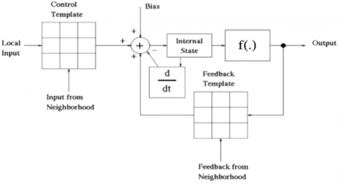
Figure 2. Global behavior of CeNN [32]
The control and feedback template matrices of the CeNN model are A and B, respectively, and T works as a bias vector. Eq. (22) converted in the CeNN form according to Eq. (24) as
$c^{*} \frac{d I_{(p, q)}}{d t}=\frac{-I_{(p, q)}}{R_{x}}+$
$\sum_{\varsigma(k, l) \in N_{r}(p, q)} A(p, q ; k, l) I_{(k, l)}(t)$
$+\sum_{\varsigma(k, l) \in N_{r}(p, q)} B(p, q ; k, l) I_{y(k, l)}(t)+T$ (25)
where, $I_{(p, q)}(t)=d(p, q, t)$ and $N_{r}$ denotes the neighborhood of finite radius $r$ of state variable $I_{(p, q)}$. Eq. (25) associated the
$\mathrm{CeNN} \quad(22)$ with $c^{*}=1, \frac{1}{R_{x}}=1$ and $T=$ $\lambda_{1}\left(\begin{array}{c}X_{1}(x, y, t) \\ -X_{2}(x+d, y, t)\end{array}\right) \frac{X_{2}(x+\Delta x, y, t)-X_{2}(x, y, t)}{\partial x}$.
The transformation templates of Eq. (25) are computed as
$\begin{gathered}A=\left[\begin{array}{ccc}0 & \alpha d N & 0 \\ \alpha d W & -\alpha(d N+d S+d W+d E) & \alpha d E \\ 0 & \alpha d S & 0\end{array}\right], \\ B=\left[\begin{array}{ccc}0 & 1 & 0 \\ 1 & -4 & 1 \\ 0 & 1 & 0\end{array}\right] .\end{gathered}$
For our proposed CeNN model, the output function is defined as $I_{y(p, q)}=I_{x(p, q)} .$ The components of $I_{(p, q)}$ denoting the position of all cells are included in the complete CeNN-processor model. The model in Eq. (25) is a network of first-order ordinary differential Eqs. According to Figure 2, the CeNN model consists of 3x3 template matrix A, which serves as the input vector $I_{(p, q)}$ as well as control template, and 3X3 template matrix B acts as a feedback template. In the model, the added bias vector is T, and all the computations are performed with the internal state. After the whole process, we obtain the output function of $I_{y(p, q)}$. The output function is similar to the input vector for our model, which shows the output vector's differentiability. The overall mapping procedure is designed so that the ordinary differential equation is represented in terms of the components of state space, and template matrices have been computed based on the best possible mapping conditions. The proposed templates A, B are defined according to the desired disparity. The obtained templates matrices of the governing CeNN array are space invariant. The MATLAB solver ode45 is used for numerical computation. Algorithm 1 gives an overview of the overall framework of the proposed approach.
Algorithm 1: Numerical implementation
Input: Initial disparity $d_{0}(x, y)$ at $\mathrm{t}=0$, choose $\alpha=0.1$, time step size $\Delta t=0.1, t_{\max }$ final time(s).
Output: Restored disparity image $d(x, y)$
1. Set $t=0$, the initial image $d(x, y, 0)$ at $t=0, t_{\text {max }}$;
2. Compute template matrices A,B and T;
3. Call CeNN function $\frac{\partial d(x, y, t+\Delta t)}{\partial t}=-d(x, y, t)+A * d(x, y, t)+B *$$d_{y}(x, y, t)+T$ and compute the next iteration $d(x, y, t+\Delta t)$;
4. Update templates A and B and goes to step 3 until tmax;
5. Return image d(x,y) at a time tmax.
The iterative CeNN scheme needs to be convergent. In this study, the convergence of algorithm 1 is proved by showing the conditions on templates A, B, and output function $d(x, y, t)$.
Definition: An autonomous dynamical system, expressed by the state equation:
$\frac{d x}{d t}=f(x), x \in \mathbb{R}^{n}$ (26)
and $f: \mathbb{R}^{n} \rightarrow \mathbb{R}^{n}$ is said to be stable almost everywhere (or convergent), if for each initial condition $x_{0} \in \mathbb{R}^{n}$ satisfies $\lim _{t \rightarrow \infty} x\left(t, x_{0}\right)=C$ (constant).
Theorem 11 [34] states that: a sufficient condition for the stability almost everywhere (convergent) of a space-invariant CeNN system, described by state Eq. (24) with strictly monotonic and a differentiable output function; is that the template is cell-linking or strictly sign-symmetric [35] (i.e. $B_{i, j} B_{-i,-j}$) and that all the template entries satisfy one of the following set of inequalities:
$\forall(i, j) \neq(0,0), B_{i, j} \geq 0$
$\forall(i, j) \neq(0,0),(-1)^{i} B_{i, j} \geq 0$
$\forall(i, j) \neq(0,0),(-1)^{j} B_{i, j} \geq 0$
$\forall(i, j) \neq(0,0),(-1)^{i+j} B_{i, j} \geq 0$ (27)
For our CeNN system, the output function of state Eq. (25), $\left(I_{y}(i, j)=I_{x}(i, j)=d_{i, j}\right)$ is linear, which is a strictly monotonic and differentiable function, and template entries of B are
$B_{0,0}=-4, B_{-1,0}=1, B_{1,0}=1, B_{0,-1}=1$
$B_{0,1}=1, B_{-1,-1}=0, B_{-1,1}=0, B_{1,-1}=0$ (28)
and $B_{1,1}=0$ satisfies the cell-linking property as $B_{-1,0} B_{1,0}>0, B_{0,-1} B_{0,1}>0, B_{-1,-1} B_{1,1}>0, B_{-1,1} B_{1,-1}>0$; and also, all the template entries satisfy the first inequality-1. Based on the above, the proposed CeNN iteration converges to the restored image $d(x, y)$.
In this section, we have presented the numerical results obtained by the CeNN approach on different images. The initial disparity is calculated by using the belief propagation method. The structure of the proposed scheme is efficient and easy to implement. The proposed method's accuracy is estimated using the bad-matching percentage (BMP) and the root-mean-square error (RMSE) matrices. For BMP and RMSE calculation, we need the ground truth data. Mathematically, the RMSE is defined between the ground truth disparity map $d_{G}(x, y)$ and the estimated disparity map $d_{e}(x, y)$ as,
$R M S E=\left\{\frac{1}{N} \sum_{(k, l)}\left[d_{e}(k, l)-d_{G}(k, l)\right]^{2}\right\}^{1 / 2}$ (29)
where, N is the total number of matching pixels.
Zitnick and Kanade [36] have introduced the BMP of the obtained disparity map. The BMP shows the rate of incorrect disparities. The disparity that differs from the image of the ground truth by pixel 1 is considered correct.
The percentage of BMP is defined as
$B M P=\left\{\frac{1}{N} \sum_{(k, l)}\left(\left|d_{e}(k, l)-d_{G}(k, l)\right|\right)>\delta\right\}$ (30)
where, $\delta$ is the disparity error tolerance.
4.1 Data collection
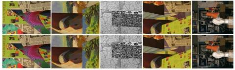
Parameter $\lambda_{1}, \alpha$ and time steps $\Delta t$ are taken for implementation in this model. The choice of $\lambda_{1}$ and $\alpha$ are not case sensitive for different images. The value of parameters fixed for all the images, and these parameters' values are $\lambda_{1}=0.2$ and $\alpha=0.8$. We have taken five Middlebury stereo benchmark images with ground truth disparity left and the right frame of images; Poster, Venus, Map, Tsukuba, and Lamp. The original images are shown in Figure 3. We have compared our RMSE and BMP values with block matching (BM) [37], simple block matching (SB) [38], block matching with dynamic programming (BMDP) [39], stereo matching with belief propagation (SMBP) [31] models for two different values 1, 0.1 of $\delta$. The initial disparity is computed as in subsection 2.2. We used a classic stereo pair whose exact disparity is known.
4.2 Qualitative and quantitative results
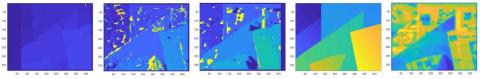
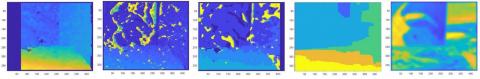
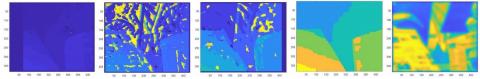
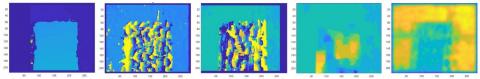
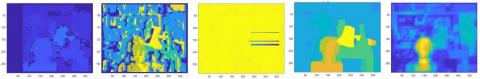
Tables 1, 2, 3, 4, and 5 list the RMSE and BMP values for the time step $\Delta t=0.1$. The numerical values have shown our results' effectiveness and claim that the proposed model preserves the edges well. The performance of BM, SB, BMDP, and SMBP methods belongs to the average results for both RMSE and BMP values, but the RMSE values of the block matching method are not desired effective. Alternatively, it could only mean that the proposed method produces the best results in RMSE and BMP. The regularization algorithm suppresses the main errors in blockage. The neighborhood properties of the CeNN algorithm have led to good BMP results. The visual effects of estimated disparity have been shown in Figures 4, 5, 6, 7, and 8. The proposed visual results are compared with the traditional methods BM [37], SB [38], BMDP [39], SMBP [31]. Figure 3 shows the five different tests for left and right images. The capturing sequence of these paintings is made up of some posters or pictures with cut-out edges. Figures 4, 5, 6 display the Poster, Tsukuba, and Venus images' visual results, respectively, and obtained the required planar scenes in the disparity map. The disparity of the monochromatic map is shown in Figure 7. In Figure 8, the obtained inequality map clearly shows the transfer to the Lamp and Head pixels. It is clearly evident that the proposed methodology did not suffer to preserve edges. The proposed method achieves a statistically significant improved visuality compared to SB and BMDP methods. The depth discontinuity of edges preserves in our suggested results and contains no extra information.
Table 1. Comparison of RMSE and BMP values for Poster image between BM [37], SB [38], BMDP [39], SMBP [31], and proposed method
|
Poster BM [37] SB [38] BMDP [39] SMBP [31] Proposed |
|
RMSE2.9342 4.12083.3396 3.58130.5667 |
|
BMP $\delta$= 0.1 0.78911 1 1 0.6920 $\delta$= 1 0.7478 0.8037 0.7126 0.9951 0.0256 |
Table 2. Comparison of RMSE and BMP values for Venus image between BM [37], SB [38], BMDP [39], SMBP [31], and proposed method
|
Venus BM [37] SB [38] BMDP [39] SMBP [31] Proposed |
|
RMSE2.29286.08132.84073.20040.5257 |
|
BMP $\delta$= 0.10.78070.9992 0.9988 0.99980.5203 $\delta$= 1 0.72450.7917 0.6991 0.99510.0044 |
Table 3. Comparison of RMSE and BMP values for Map image between BM [37], SB [38], BMDP [39], SMBP [31], and proposed method
|
Map BM [37] SB [38] BMDP [39] SMBP [31] Proposed |
|
RMSE6.7882 6.78826.7584 5.4047 0.7936 |
|
BMP $\delta$= 0.1 0.6416 0.9966 1 0.99970.8465 $\delta$= 1 0.64010.8282 0.74520.98990 |
Table 4. Comparison of RMSE and BMP values for Tsukuba image between BM [37], SB [38], BMDP [39], SMBP [31], and proposed method
|
Tsukuba BM[37] SB[38] BMDP[39] SMBP[31] Proposed |
|
RMSE1.8269 3.48543.4891 2.8027 0.1619 |
|
BMP $\delta$= 0.1 0.7885 1 1 1 0.4121 $\delta$= 1 0.5249 0.6825 0.47020.90080 |
Table 5. Comparison of RMSE and BMP values for Lamp image between BM [37], SB [38], BMDP [39], SMBP [31], and proposed method
|
Lamp BM [37] SB [38] BMDP [39] SMBP [31] Proposed |
|
RMSE7.4729 7.3585 7.75197.7344 0.2989 |
|
BMP $\delta$= 0.1 0.6909 0.9190 0.89920.9939 0.8402 $\delta$= 1 0.6904 0.8264 0.83850.99390 |
Table 6. Taken time for the proposed algorithm computation
|
Images Time (s) |
|
"Poster"75.249 "Venus"76.5735 "Map" 20.2213 "Tsukuba" 69.2015 "Head_Lamp"27.2172 |
Figure 3. We have shown five different tests for left and right images (first row for left images and second row for right images). The images are shown in the first column: Poster; second column: Tsukuba; third column: Map; fourth column: Venus; last column: Lamp
Figure 4. The computed disparity for Poster image using BM [37], SB [38], BMDP [39], SMBP [31], and the proposed method are given from left to right, respectively
Figure 5. The computed disparity for Tsukuba image using BM [37], SB [38], BMDP [39], SMBP [31], and the proposed method are given from left to right, respectively
Figure 6. The computed disparity for Venus image using BM [37], SB [38], BMDP [39], SMBP [31], and the proposed method are given from left to right, respectively
Figure 7. The computed disparity for Map image using BM [37], SB [38], BMDP [39], SMBP [31], and the proposed method are given from left to right, respectively
Figure 8. The computed disparity for Head_Lamp image using BM [37], SB [38], BMDP [39], SMBP [31], and the proposed method are given from left to right, respectively
To show the overall performance, the computational time has been shown. The operation time of the proposed model on MATLAB R2018a on the desktop with an i5 processor, 8GB RAM are listed in Table 6. The other methods are executed under different conditions. Therefore, it might not be possible to compare the proposed method's computational efficiency with other methods.
In the proposed method, a significant time step can be used for solving the PDE. The numerical results ignite that the proposed scheme can deal with different boundary conditions, nonlinear properties, and complex geometry with a simple and efficient approach. However, when comparing our results to state-of-the-art studies, it must be pointed out that the proposed method easy to implement and preserves depth discontinuity. Our results cast a new light on disparity estimation through CeNN.
The variation in illumination is always non-uniform and located in between the left and right images. There are various real and difficult situations in which we cannot avoid non-uniform illumination differences between stereo images. Energy minimization approaches are not sensitive to non-uniform illumination differences, though they provide good results by locating local minima over large areas. The energy minimization algorithm has been proposed to provide a disparity map as an output from the illuminated variant stereo pair. The energy minimization approach's computational cost is very high and may not be cost-wise suitable for real-time applications. The proposed model decreases the computation cost and is highly effective on non-uniform illumination due to its structure. The disparity map obtained using the energy minimization approach can reconstruct the 3D surface, and the obtained reconstructed results are close to the real depth information.
The proposed PDE estimates the disparity maps of the images by preserving the discontinuity between different regions without any parameter settings. This was achieved by converting the prepared PDE into CeNN form using the finite difference method, and the obtained template matrices serve as the transformation matrices. The obtained CeNN system allows the use of significant time steps to reduce the number of iterations and computation time while maintaining sufficient numerical accuracy. The convergence of the numerical scheme has been proved, and the proposed algorithm is easily implemented with low computation costs. Therefore, the numerical results of the proposed algorithm are highly competitive with the other state-of-the-art algorithms with respect to the ground truth values. The numerical results showed that the proposed algorithm obtained improved RMSE and BMP values and a sharp spatially correlated disparity vector field. The limitation of the proposed scheme is the computational load to define PDE. The improvement in the algorithm for the disparity of the quadric surfaces is needed for further research. In the future, one can investigate the optical flow and multiview reconstruction using a dense matching approach.
One of the authors, Mahima, is thankful for the support of the University Grant Commission (UGC) during her Ph.D. through Ref. No. 412261.
[1] Faugeras, O., Faugeras, O.A. (1993). Three- Dimensional Computer Vision: A Geometric Viewpoint. MIT Press.
[2] Grimson, W.E.L. (1985). Computational experiments with a feature based stereo algorithm. IEEE Transactions on Pattern Analysis and Machine Intelligence, 7(1): 17-34. https://doi.org/10.1109/TPAMI.1985.4767615
[3] Nasrabadi, N.M. (1992). A stereo vision technique using curve-segments and relaxation matching. IEEE Transactions on Pattern Analysis and Machine Intelligence, 14(5): 566-572. https://doi.org/10.1109/34.134060
[4] Robert, L., Faugeras, O.D. (1991). Curve-based stereo: Figural continuity and curvature. Proceedings. 1991 IEEE Computer Society Conference on Computer Vision and Pattern Recognition, Maui, HI, USA, pp. 57-58. https://doi.org/10.1109/CVPR.1991.139661
[5] Devernay, F., Faugeras, O.D. (1994). Computing differential properties of 3-D shapes from stereoscopic images without 3-D models, Seattle, WA, USA, pp. 208-213. https://doi.org/10.1109/CVPR.1994.323831
[6] Fua, P. (1993). A parallel stereo algorithm that produces dense depth maps and preserves image features. Machine Vision and Applications, 6(1): 35-49. https://doi.org/10.1007/BF01212430
[7] Nishihara, H.K. (1984). Practical real-time imaging stereo matcher. Optical Engineering, 23(5): 235536. https://doi.org/10.1117/12.7973334
[8] Fleet, D.J., Jepson, A.D. (1990). Computation of component image velocity from local phase information. International Journal of Computer Vision, 5(1): 77-104. https://doi.org/10.1007/BF00056772
[9] Fleet, D.J., Jepson, A.D. (1993). Stability of phase information. IEEE Transactions on Pattern Analysis and Machine Intelligence, 15(12): 1253-1268. https://doi.org/10.1109/34.250844
[10] Kumar, S., Kumar, S., Sukavanam, N., Raman, B. (2014). Dual tree fractional quaternion wavelet transform for disparity estimation. ISA Transactions, 53(2): 547-559. https://doi.org/10.1016/j.isatra.2013.12.001
[11] Wiklund, J., Westelius, C.J., Knutsson, H. (1992). Hierarchical phase based disparity estimation. Linköping University, Department of Electrical Engineering
[12] Alvarez, L., Deriche, R., Sanchez, J., Weickert, J. (2002). Dense disparity map estimation respecting image discontinuities: A PDE and scale-space based approach. Journal of Visual Communication and Image Representation, 13(1-2): 3-21. https://doi.org/10.1006/jvci.2001.0482
[13] Barnard, S.T. (1989). Stochastic stereo matching over scale. International Journal of Computer Vision, 3(1): 17-32. https://doi.org/10.1007/BF00054836
[14] Bascle, B., Deriche, R. (1993). Energy-based methods for 2D curve tracking, reconstruction, and refinement of 3D curves and applications. Geometric Methods in Computer Vision II, 2031: 282-293. https://doi.org/10.1117/12.146633
[15] Kolmogorov, V., Zabin, R. (2004). What energy functions can be minimized via graph cuts? IEEE Transactions on Pattern Analysis and Machine Intelligence, 26(2): 147-159. https://doi.org/10.1109/TPAMI.2004.1262177
[16] Heitz, F., Pérez, P., Bouthemy, P. (1994). Multiscale minimization of global energy functions in some visual recovery problems. CVGIP: Image Understanding, 59(1): 125-134. https://doi.org/10.1006/ciun.1994.1008
[17] Kim, H., Sohn, K. (2003). Hierarchical disparity estimation with energy-based regularization. Proceedings 2003 International Conference on Image Processing (Cat. No. 03CH37429), Barcelona, Spain. IEEE. https://doi.org/10.1109/ICIP.2003.1246976
[18] Shah, J. (1993). A nonlinear diffusion model for discontinuous disparity and half-occlusions in stereo. In Proceedings of IEEE Conference on Computer Vision and Pattern Recognition, New York, USA pp. 34-40. https://doi.org/10.1109/CVPR.1993.341004
[19] Min, D., Sohn, K. (2006). Edge-preserving simultaneous joint motion-disparity estimation. 18th International Conference on Pattern Recognition (ICPR'06), pp. 74-77. https://doi.org/10.1109/ICPR.2006.470
[20] Robert, L., Deriche, R. (1996). Dense depth map reconstruction: A minimization and regularization approach which preserves discontinuities. European Conference on Computer Vision, UK, pp. 439-451. https://doi.org/10.1007/BFb0015556
[21] Ozanian, T. (1995). Approaches for stereo matching. Modeling, Identification and Control, 16(2): 65-94. https://doi.org/10.4173/mic.1995.2.1
[22] Rao, J. (2010). Adaptive contextual regularization for energy minimization based image segmentation. Doctoral dissertation, University of British Columbia.
[23] Ayache, N. (1987). Fast and reliable passive trinocular stereo vision. Proc. of First Int'l Conf. on Computer Vision, pp. 422-427.
[24] Ohta, Y., Kanade, T. (1985). Stereo by intra-and inter-scanline search using dynamic programming. IEEE Transactions on Pattern Analysis and Machine Intelligence, 7(2): 139-154. https://doi.org/10.1109/TPAMI.1985.4767639
[25] Pollard, S.B., Mayhew, J.E., Frisby, J.P. (1985). PMF: A stereo correspondence algorithm using a disparity gradient limit. Perception, 14(4): 449-470. https://doi.org/10.1068%2Fp140449
[26] Fleet, D.J., Jepson, A.D., Jenkin, M.R. (1991). Phase-based disparity measurement. CVGIP: Image Understanding, 53(2): 198-210. https://doi.org/10.1016/1049-9660(91)90027-M
[27] Kim, H., Choe, Y., Sohn, K. (2004). Disparity estimation using a region-dividing technique and energy-based regularization. Optical Engineering, 43(8): 1882-1891. https://doi.org/10.1117/1.1766299
[28] Deriche, R., Bouvin, C., Faugeras, O.D. (1997). Level-set approach for stereo. Investigative Image Processing, 2942: 150-161. https://doi.org/10.1117/12.267171
[29] Kim, H., Kim, S., Son, J., Sohn, K. (2001). Feature-based disparity estimation for intermediate view reconstruction of multiview images. International Conference on Imaging Science, Systems and Technology.
[30] Li, C., Xu, C., Gui, C., Fox, M.D. (2010). Distance regularized level set evolution and its application to image segmentation. IEEE Transactions on Image Processing, 19(12): 3243-3254. https://doi.org/10.1109/TIP.2010.2069690
[31] Felzenszwalb, P.F., Huttenlocher, D.P. (2006). Efficient belief propagation for early vision. International Journal of Computer Vision, 70(1): 41-54. https://doi.org/10.1007/s11263-006-7899-4
[32] Chua, L.O., Yang, L. (1988). Cellular neural networks: Theory. IEEE Transactions on Circuits and Systems, 35(10): 1257-1272. https://doi.org/10.1109/31.7600
[33] Roska, T., Chua, L.O. (1993). The CNN universal machine: an analogic array computer. IEEE Transactions on Circuits and Systems II: Analog and Digital Signal Processing, 40(3): 163-173. https://doi.org/10.1109/82.222815
[34] Paolo-Civalleri, P., Gilli, M. (1999). On stability of cellular neural networks. Journal of VLSI Signal Processing Systems for Signal, Image and Video Technology, 23(2-3): 429-435. https://doi.org/10.1023/A:1008109505419
[35] Chua, L.O., Wu, C.W. (1992). The universe of stable CNN templates. International Journal of Circuit Theory and Applications: Special Issue on Cellular Neural Networks, 20: 497-517.
[36] Zitnick, C.L., Kanade, T. (2000). A cooperative algorithm for stereo matching and occlusion detection. IEEE Transactions on Pattern Analysis and Machine Intelligence, 22(7): 675-684. https://doi.org/10.1109/34.865184
[37] Konolige, K. (1998). Small vision systems: Hardware and implementation. Robotics Research, Tokyo, Japan, pp. 203-212. https://doi.org/10.1007/978-1-4471-1580-9_19
[38] Chen, Y.S., Hung, Y.P., Fuh, C.S. (2001). Fast block matching algorithm based on the winner-update strategy. IEEE Transactions on Image Processing, 10(8): 1212-1222. https://doi.org/10.1109/83.935037
[39] Karathanasis, J., Kalivas, D., Vlontzos, J. (1996). Disparity estimation using block matching and dynamic programming. Proceedings of Third International Conference on Electronics, Circuits, and Systems, 2: 728-731. https://doi.org/10.1109/ICECS.1996.584465