Asan Ihsan Abas | Nurdan Akhan Baykan*
© 2021 IIETA. This article is published by IIETA and is licensed under the CC BY 4.0 license (http://creativecommons.org/licenses/by/4.0/).
OPEN ACCESS
Focus is limited and singular in many image capture devices. Therefore, different focused objects at different distances are obtained in a single image taken. Image fusion can be defined as the acquisition of multiple focused objects in a single image by combining important information from two or more images into a single image. In this paper, a new multi-focus image fusion method based on Bat Algorithm (BA) is presented in a Multi-Scale Transform (MST) to overcome limitations of standard MST Transform. Firstly, a specific MST (Laplacian Pyramid or Curvelet Transform) is performed on the two source images to obtain their low-pass and high-pass bands. Secondly, optimization algorithms were used to find out optimal weights for coefficients in low-pass bands to improve the accuracy of the fusion image and finally the fused multi-focus image is reconstructed by the inverse MST. The experimental results are compared with different methods using reference and non-reference evaluation metrics to evaluate the performance of image fusion methods.
particle swarm optimization, bat algorithm, Laplacian pyramid, curvelet transform, image fusion
Image fusion is a process of combining information from multiple sources like multi-focus, multi-spectral, or multi- sensor images to produce a more informative single fused image. The fused image combines two or more source images into a single fused image and has a higher information content than any of the single source images. The goal of image fusion s not only to reduce the amount of data but also to create new images that are more suitable for human visual perception.
Multi-focus image fusion is a technique that combining multiple images from the same scene with different focuses to get an all-in-one focus image by using specific fusion techniques to get more information from the fused images rather than the single image. It is used to get more quality image because the object space (depth of field) lens sensor in image device is limited and only objects that are in a certain depth remain ‘in focus’, while all other objects become ‘out of focus’. If one object in the scene is in focus, another one will be out of focus, therefore, a fusion process is required to achieve all objects in focus and all focused objects are selected [1, 2]. The multi-focus image fusion is a sub-domain of image fusion, and it is the basis of many fusion fields such as digital imaging, medical imaging, remote sensing, and machine vision [3-7].
Multi-focus image fusion methods can be divided into two categories based on spatial and transform domain. In the spatial domain, the source images are fused directly in gray level such as image fusion using weighted average value and Principal Component Analysis (PCA) [8]. In the transform domain, images are fused by frequency domain using decomposition procedure. Generally, the decomposition procedure is completed with a Multi-Scale Transform (MST) [9]. Typical transform algorithms such as Wavelet Transform (DWT) [10], Laplacian Pyramid (LP) [11], Curvelet Transform (CvT) [12], Contourlet Transform (CT) [13], Stationary Wavelet Transform [14], Nonsubsampled Contourlet Transform [15] and Nonsubsampled Shearlet Transform [16] are MST image transformations that decompose the source images into a set of sub-images to extract the detailed information. After the decomposition, the fused sub-images (coefficients) are obtained by specific fusion rules as Choosing Max (CM) and Weighted Average (WA) [17-19]. At last, the fused image is generated by inverse MST using the sub-image decomposed into a base and several detail layers. A general framework for MST image fusion is shown in Figure 1.
For fusion mainly, low-frequency information, which can control in contrast of the fused image, is used [20]. The standard fusion rule, used in many researches, is a weighted average which average the low frequency coefficient. However, the weighted average fusion rule is not suitable for all types of images because it can reduce the contrast of the fused image and sometimes may not produce the desired results. To solve this problem, some image fusion techniques based on optimization algorithms such as Particle Swarm Optimization (PSO) and Genetic Algorithm (GA) have been proposed to find out the optimum weights from extracted edges, in recent years. These algorithms are widely used in many optimization problems to get optimal solution result. In many studies of fusion, PSO is used to optimize the weights in a region-based weighted average fusion rule.
An et al. [21] presented a new multi-objective optimization method of multi-objective image fusion based on Adaptive PSO, which can simplify the multi-objective image fusion model and overcome the limitations of classic methods. Fu et al. [22], implemented an optimal algorithm for multi-Source RS image fusion. This algorithm considers the Wavelet Transform (WT) of the translation invariance as the model operator, also regards the contrast pyramid conversion as the observed operator. Then it designs the objective function by taking the weighted sum of evaluation indices and optimizes the objective function by employing genetic-iterative self-organizing data analysis algorithm to get a higher resolution of RS image. Kanmani and Narasimhan [23] proposed an optimal weighted averaging fusion strategy for images using Dual-Tree Wavelet Transform (DT-WT) and Self-Tunning PSO (STPSO). In this method, a weighted averaging fusion rule is formulated that uses to find optimal weights from STPSO for the fusion of both high and low frequency coefficients, obtained through Dual Tree DWT to fused thermal and visual images. Daniel [24] proposed an optimum wavelet-based homographic filter that provides multi-level decomposition in homographic domain using Hybrid Genetic-Grey Wolf Optimization algorithm to get optimal scale value in medical image fusion technique. Yang et al. [25], within the Non-Subsampled Shearlet Transform (NSST), presented a new multi-focus image fusion method based on a non-fixed-base dictionary and multi-measure optimization. In their work, the authors proposed an optimization method to resolve the problem blurred in some details in the focused region for the NSST. Paramanandham and Rajendiran [26], have presented a multi-focus image fusion based on Self-Resemblance Measure (SRM), consistency verification and multiple objective PSO. In this method, the multi-objective PSO is used to adaptively select the block size of the fused image. The source images are divided into blocks and evaluation metrics are used to measure the degree of focus in pixel and select correct block. To create an all-in-focus image, Abdipour and Nooshyar [27], proposed an image fusion technique in wavelet domain based on variance and spatial frequency. The variance and spatial frequency of the 16×16 blocks of wavelet coefficients were considered for measuring the contrast and identifying high clarity of the image. Then, the Consistency Verification (CV) is used to improve the fused image quality. Finally, the decision map based on the maximum selection rule is used to register the selection results.
Figure 1. A general framework for MST image fusion [19]
Image fusion methods are classified into two categories as “transform domain methods” and “spatial domain methods”. In the spatial domain methods, the source images are fused using some spatial features of images. In spatial domain methods, a fused image is obtained as the weighted average values of pixels of all the source images. The most prominent characteristic of these methods is that they do not contain the inversion step to reconstruct the fused image. However, since these methods only use spatial properties, structural properties are not used sufficiently.
The domain transform methods consist of three main stages as mage transform, coefficient fusion and inverse transform. Firstly, an image decomposition/representation approach is applied to all source images and images are converted into a transform domain. After then, the transformed coefficients taken from source images are merged by a fusion rule. Finally, an inverse transform is used on the fused coefficients for obtaining the fused image. Laplacian Pyramid and Curvelet Transform are two basic transform methods used frequently in the literature.
2.1 Laplacian pyramid (LP)
The idea of image pyramid goes back to Burt and Adelson in 1983 [28]. The principle of this method is to decompose the original image by applying the Gaussian filter and the interpolation expansion for the Gaussian Pyramid to get the multi-resolution image. LP produces the edge information detail of the image at each level. The LP decomposition is performed in two stages [2, 11, 28, 29]:
The first stage: Gaussian Pyramid decomposition.
Multi-scale images are produced by applying Gaussian filter (low-pass) by convolving the image with Gaussian weighting function (w) and then subsampling of these images. This operation is called REDUCE. The decomposition transformation of the Gaussian pyramid using discrete formulation of an image can be calculated as follows using Eq. (1).
$G_{l}(i, j)=\sum_{x=-2}^{2} \sum_{y=-2}^{2} w(x, y) \cdot G_{l-1}(2 i+x, 2 j+y)$
$l \in[1, N), i \in\left[0, X_{l}\right), j \in\left[0, Y_{l}\right)$ (1)
In Eq. (1), $G_{l}$ is Gaussian pyramid, w(x,y) is Gaussian weighting function at low pass filters. The source image in the initial layer is the $G_{0}$ and N is the number of the Gaussian layers; $X_{l}$ and Yl represented the number of columns and rows in the ith layers of pyramid.
The second stage: Laplacian Pyramid decomposition.
The LP is obtained by computing the convolving difference between the adjacent level of the Gaussian Pyramid. This operation is called EXPAND. LP produces the edge information detail of the image at each level and consisting of layers as given Eq. (2).
$L P_{L}=f(x)=\left\{\begin{array}{c}G_{l}-G_{l+1}^{*}, L \in[0, L) \\ G_{l}, l=L\end{array}\right.$ (2)
In Eq. (2), $G_{l+1}^{*}$ is Gaussian expanded of $G_{l}$. LPL is Laplacian pyramid and l is the l-th level decomposed; L is the number of LP levels.
Reconstruction image is obtained by adding layers of the pyramid. The inverse transformation is given in Eq. (3).
$G_{l}(i, j)=4 \sum_{x=-2}^{2} \sum_{y=-2}^{2} w(x, y) G_{l+1}\left(\frac{i+x}{2}, \frac{j+y}{2}\right)$ (3)
In this paper, firstly LP is used as MST. For this aim, the LP transform was subjected to obtain the pyramid levels of images (Figure 2). A low level of the pyramid contains high quality information of the image. For fusion; while "the adaptive region average gradient weighted rule" was used for low levels of the pyramid, "choose max with consistency check rule" was used for high levels of the pyramid. After the fusion, the fused image is obtained by applying the inverse LP transform.
Figure 2. Laplacian pyramid transform
Standard image fusion approach using LP is summarized below:
2.2 Curvelet transform (CvT)
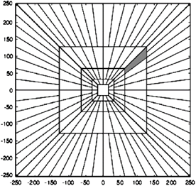
Curvelet transform, a multi-scale directional transform, is used to represent the image at different angles and scales. It is developed by Candès and Donoho to solve the problem limitation of Wavelet and Gabor transform [30] (Figure 3).
There are two types of CvT called first and second generation. Although the first generation Curvelet is used effectively to remove noise from images, it requires more processing time compared to the second generation. Also, the numerical application of the first generation CvT is quite complex. The second generation CvT can be applied in a shorter time, with less operation and in a simpler way.
The first generation CvT, proposed based on an anisotropic geometric wavelet called Redgilet transform, is decomposed the image into a set of wavelet bands and to analyze each band by a local ridgelet transform.
Figure 3. Curvelet transform
In this work second generation 2D Fast Discrete Curvelet Transform version implemented via ‘‘wrapping” transform (FDCT-Wrap) that utilizes fast Fourier Transform and proposed by Candès et al. in 2006 was used [31]. This method is faster and more robust than Curvelet based on Ridgelet.
In the frequency domain decomposition, it adopts local Fourier transform and is applied at four steps (FDCT-Wrap):
$\hat{f}[i, j],-\frac{n}{2} \leq i, j<\frac{n}{2}$ (4)
In Eq. (4), $\hat{f}[i, j]$ is the Fourier coefficients and i, j is the index of the pixel image; n is Fourier sample.
$\hat{f}[i, j]=\hat{f}\left[i, j-i * \tan \theta_{i}\right] \times \widehat{U}[i, j]$ (5)
In Eq. (5), θ is orientation in the range $\left(-\frac{\pi}{4}, \frac{\pi}{4}\right)$ and $\widehat{U}$ is parabolic window.
The CvT divides the image into three parts as the coarsest layer, detail layer and finest layer. The coarsest layer is the low-frequency sub image information and represents the main information of the image. The finest layer contains the high-frequency sub-images information and noise which reflects the details components and detail layer contains the strong edge details information of the source image from different directions and scales [32]. Commonly for the fusion, while an average or weighted average rule is used in the low-frequency sub image, the maximum absolute rule is often used in the high frequency sub image.
Standard image fusion approach using CvT is summarized below:
3.1 Particle Swarm Optimization (PSO)
PSO is a stochastic optimization and an evolutionary computational technique that is able to simulate the social behavior of bird flocking or fish [33]. It was introduced by Kennedy and Eberhart in 1995 to find the parameters that provide the minimum or maximum value of an objective function. PSO works by having a population called as “swarm”. Each candidate solution of the swarm is called a “particle” and each particle is moved around in the search space by their own “velocity”. The velocity $\left(V_{i}\right)$ is the distance travelled by the particle from one position to the current position $\left(x_{i}\right)$. The concepts of velocity and position are used by PSO algorithms in order to find the optimal point(s) in working space.
In PSO, each particle affected by its personal best achieved position ($p_{\text {best }}$) and the group global best position ($g_{\text {best }}$) (solution of the problem). The velocity and position are updated using Eq. (6) and Eq. (7) [33]:
$V_{i}^{k+1}=w \times V_{i}^{k}+c_{1} \times$ rand $\times\left(P_{\text {best } i}^{k}-X_{i v}^{k}\right)+$
$c_{2} \times$ rand $\times\left(g_{\text {best }}{ }^{k}-X_{i}^{k}\right)$ (6)
$X_{i}^{k+1}=X_{i}^{k}+V_{i}^{k+1}, i=1,2, \ldots . n$ (7)
In Eq. (6) and (7), $V_{i}^{k+1}$ is velocity and $X_{i}^{k+1}$ is a position of $i^{t h}$ particle in iteration $k+1$. $P_{\text {best }}$ is the best value of fitness function achieved by $i^{t h}$ particle before iteration k and $g_{\text {best }}$ is the best fitness function value achieved so far by any particle. $c_{1}$ and $c_{2}$ acceleration coefficients, rand is a random variable between [0, 1], and w is represented the inertia weight factor used to provide well-balanced mechanism between global and local exploration abilities. PSO pseudo-code is described in Algorithm 1.
|
Algorithm 1. Pseudo-code of the PSO algorithm |
|
3.2 Bat algorithm (BA)
Bat algorithm was developed by Xin-She Yang in 2010 for global optimization. It is a metaheuristic algorithm inspired by the echolocation system of the bats and it simulates the behaviors a swarm bat uses to find prey/food [34]. Just like particles in PSO, also bats in the algorithm have velocity and position and they are updated using the Eq. (8-10) [35, 36].
In Eq. (8), (9) and (10); β is a random vector in a range [0, 1], the frequency f is in a range $\left[f_{\min }, f_{\max }\right]$ indicates the best global value at a time and $x_{*}$ is the velocity change at position $x_{i}$ in iteration $t^{t h}$.
The BA pseudo-code is given in Algorithm 2.
$f_{i}=f_{\min }+\left(f_{\max }-f_{\min }\right) \beta$ (8)
$v_{i}^{t}=v_{i}^{t-1}+\left(x_{i}^{t-1}-x_{*}\right) f_{i}$ (9)
$x_{i}^{t}=x_{i}^{t-1}+v_{i}^{t}$ (10)
On the echolocation system, bats calculate the distance to their target and transmit with signals of loudness (A) and wavelength (λ) while flying towards their prey. The frequency value in the BAT algorithm allows the pace and ranging of the bat movements to be determined. In the algorithm when bats approach their prey; A decreases, the pulse emission rate r increases, $\alpha$ and $\gamma$ are constants.
|
Algorithm 2. Pseudo-code of the BA |
|
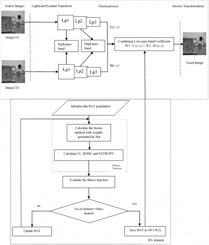
In this work, to enhance the contrast preserving the overall brightness of the fused image, a novel multi-scale fusion method based on Bat Algorithm (BA) that aims to find optimal weights was proposed. Firstly, a specific MST (Laplacian Pyramid or Curvelet Transform) on the two source images to obtain their low-pass and high-pass bands was performed. Secondly, BA was used to find out the optimum weights for coefficients in low-pass bands to improve the accuracy of the fusion whereas in high-frequency domain, the absolute maximum rule was used as given in the literature. Finally, the fused multi-focus image was reconstructed by the inverse MST. In order to test the performance of BA; PSO which is used in the literature, was also used and the results were compared.
4.1 Proposed fusion method
The fusion process is categorized into 2 parts as spatial and frequency domain. The two employed MST methods used in the frequency domain are CvT and LP transforms. In this study, CvT or LP was used, and fusion was made in the frequency domain. While the pixel values of two source images are added as the pixel value in the fused image in the spatial domain, the process in the frequency domain is different. In the frequency domain, a multi-scale transformation is applied to the source images to obtain the transformation space coefficients. Then, the image merge rules (fusion rules max and average) are applied using the coefficients and finally reverse transformation is performed to obtain the fusion image [37, 38].
For image fusion, first, the source images are decomposed to low-frequency and high-frequency sub-band of images with one of the MST methods. The high-frequency sub-band images reflect the details components and contain the edge details information of the source image from different directions and scales. On the other hand, the low-frequency sub-band images denote the approximate component, which represents the main information of the source image. After the decomposition, in the high-frequency domain the fusion rule of each image coefficient is the absolute maximum rule Eq. (11) whereas in the low-frequency domain, an average or weighted average rule is commonly used in Eq. (12).
$C F_{i j}^{H}=\left\{\begin{array}{l}C A_{i j}^{H}, C A_{i j}^{H}>C B_{i j}^{H} \\ C B_{i j}^{H}, C A_{i j}^{H}<C B_{i j}^{H}\end{array}\right.$ (11)
In Eq. (11), $C F_{i j}^{H}$ is high-frequency fusion image coefficient, $C A_{i j}^{H}$ and $C B_{i j}^{H}$ are high-frequency source images coefficients.
$C F_{i j}^{L}=\frac{1}{2}\left(C A_{i j}^{L}+C B_{i j}^{L}\right)$ (12)
In Eq. (12), $C F_{i j}^{L}$ is a low-frequency fusion image coefficient, $C A_{i j}^{L}$ and $C B_{i j}^{L}$ are low-frequency source images coefficients.
The fusion rules are very important for the quality of fusion because they control the contrast and intensity of a fused image. Therefore, a new fusion rule for the low frequency band is proposed in this study to obtain better images in fusion. Instead of averaging the coefficients of the source images in the low frequency band, image-based adaptive weighted coefficients using metaheuristic algorithms were generated as in Eq. (13).
$C F_{i j}^{L}=\frac{\left(w_{1} \times C A_{i j}^{L}+w_{2} \times C B_{i j}^{L}\right)}{w_{1}+w_{2}}$
$\quad$ where $w \in(0,1)$ (13)
The optimization algorithm is aimed to get $w_{1}$ and $w_{2}$ that are maximizing the correlation coefficient (CC) as in Eq. (14) and Entropy (EN) as in Eq. (15) while minimizing the Root Mean Square Error (RMSE) as in Eq. (16).
$C C=1 / 2\left(\begin{array}{c}\frac{\sum_{i=1}^{M} \sum_{j=1}^{N}\left(I_{1}(i, j)-\bar{I}_{1}\right)(F(i, j)-\bar{F})}{\sqrt{\sum_{i=1}^{M} \sum_{j=1}^{N}\left(I_{1}(i, j)-\bar{I}_{1}\right)^{2}} \sqrt{\sum_{i=1}^{N} \sum_{j=1}^{M}(F(i, j)-\bar{F})^{2}}}+ \\ \frac{\sum_{i=1}^{M} \sum_{j=1}^{N}\left(I_{2}(i, j)-\bar{I}_{2}\right)(F(i, j)-\bar{F})}{\sqrt{\sum_{i=1}^{M} \sum_{j=1}^{N}\left(I_{2}(i, j)-\bar{I}_{2}\right)^{2}} \sqrt{\sum_{i=1}^{N} \sum_{j=1}^{M}(F(i, j)-\bar{F})^{2}}}\end{array}\right)$ (14)
In Eq. (14), $I_{1}(i, j)$ and $I_{2}(i, j)$are the references and F(i,j) is the fused image at the gray-level value. I and F are the average gray-level values, respectively and M, N are the sizes of the input image.
$E N=-\sum_{i=0}^{L-1} p_{i} \log _{2}\left(p_{i}\right)$ (15)
$R M S E=1 / 2\left(\begin{array}{c}\sqrt{\frac{1}{M \times N} \sum_{i=1}^{M} \sum_{j=1}^{N}\left(\left(I_{1}(i, j)\right)-F(i, j)\right)^{2}}+ \\ \frac{1}{\overline{M \times N} \sum_{i=1}^{M} \sum_{j=1}^{N}\left(\left(I_{2}(i, j)\right)-F(i, j)\right)^{2}}\end{array}\right)$ (16)
In Eq. (15), i is the probability density of the grayscale of a pixel value i and L is the number of intensity levels in the image, $p_{i}$ is pixel value. In Eq. (16), $I_{1}, I_{2}$ are source images and $F$ is a fused image. M, N are the size of the input image and (i, j) are image coordinates.
In this study, a multi-objective function as linear combination was used (Eq. (17)). While $f_{1}(X), f_{2}(X), f_{3}(X)$ point to three objectives functions, a new (general) objective function has been created for multi-objective optimization [39].
$f(X)=\alpha_{1} f_{1}(X)+\alpha_{2} f_{2}(X)+\alpha_{3} f_{3}(X)$ (17)
In other words, $\forall \alpha_{i}$ is scalar weights denoted for multi objective function [40]. In Eq. (17); $f_{1}$ for CC, $f_{2}$ for EN, $f_{3}$ for (1/RMSE) are three objective functions; $\alpha_{1}, \alpha_{2}, \alpha_{3}$ are constant value indicates relative importance that of one objective function relative to the others. In our study, $\alpha_{1}, \alpha_{2}, \alpha_{3}$ were tested for different values and the best fusion results were found when $\alpha_{1}=\alpha_{2}=0.25$ and $\alpha_{3}=0.5$ according to the weighted sum of multi-objective function based on [41]. Then this optimal values as an optimal weight was used during fusion of low band coefficient to get the fused image.
To obtain the optimal weighted coefficients for optimal fused image, the BA parameters in Table 1 selected. In BA, each BAT is represented as a candidate solution to the optimization problem and represented by a two-dimensional search space that each corresponds to one of the two weights. The solution set that maximizes the objective function is stored as “$g_{\text {best }}$. The best of the “$g_{\text {best }}$” value are the $w_{1}$ and $w_{2}$ optimal weights, which together maximize the correlation coefficient and entropy while minimizing the Root Mean Square Error (RMSE). $w_{1}$ and $w_{2}$ weights can take values between 0 and 1 ([0, 1]) so that their sum is 1. In the fusion process, obtained optimized weights getting from metaheuristic algorithms were used to fuse the low-frequency coefficients obtained by applying MST transform.
In Figure 4, image fusion steps for low frequency coefficients with CvT based on PSO are given. Steps are the same also for BA.
Also, in Algorithm 3, pseudo-code of fusion process with PSO is given.
|
Algorithm 3. Steps of the image fusion using PSO |
|
In Figure 5, image fusion steps for low frequency coefficients with LP based on BA are given. Steps are the same also for PSO. Also, at Algorithm 4, pseudo-code of fusion process with BA is given.
Figure 4. The image fusion process step with CvT based on PSO algorithm
Figure 5. The image fusion process step with LP based on BA
|
Algorithm 4. Steps of the image fusion using BA |
|
4.2 Dataset
For testing, multi-focus gray scale images were used to verify the success of the method. The images were taken from Image Fusion Dataset [42]. The images’ dataset in gray scale format and have different size. There are a total of 93 images in the dataset.
We tested our method on the multi-focus gray scale images [42]. For fusion, parameters of the PSO and BA are given in Table 1 below.
Table 1. Parameters of PSO and BA for fusion
|
Parameter value |
PSO |
BA |
|
Population size (s) |
40 |
40 |
|
Inertia weight (w) |
0.1 |
X |
|
Max. Iteration (iter) |
40 |
40 |
|
Learning constants |
Constants $c_{1}=c_{2}=2$ |
X |
|
Parameter value Frequency |
X |
Frequencies $f_{\min }=0, f_{\max }=2$ |
|
Initial Pulse rate (r) |
X |
0.5 |
|
Initial Loudness (A) |
X |
0.25 |
X: Not parameter value
The performance of the developed fusion technique has been compared with the classical methods and fused images are evaluated quantitatively by employing reference-based metrics. The definitions of metrics are as follows:
$R M S E=\sqrt{\frac{1}{M \times N} \sum_{i=1}^{M} \sum_{j=1}^{N}((R(i, j))-F(i, j))^{2}}$ (18)
In Eq. (18), R(i,j), F(i,j) are reference and fused image; $N x M$ is the size of the input image.
$C C=\frac{\sum_{i=1}^{M} \sum_{j=1}^{N}(I(i, j)-\bar{I})(F(i, j)-\bar{F})}{\sqrt{\sum_{i=1}^{M} \sum_{j=1}^{N}(I(i, j)-\bar{I})^{2}} \sqrt{\sum_{i=1}^{N} \sum_{j=1}^{M}(F(i, j)-\bar{F})^{2}}}$ (19)
In Eq. (19), I(i,j) is the reference image and F(i,j) is the fused image at the gray-level value. I and F are the average gray-level value, respectively and M x N is the size of the input image.
$P S N R=10 \log \frac{(L-1)^{2}}{R M S E^{2}}$ (20)
In Eq. (20), L is the number of the gray levels of the image; RMSE is the root mean square error.
$E=-\sum_{i=0}^{L-1} p_{i \log _{2}\left(p_{i}\right)}$ (21)
In Eq. (21), i is the probability density of the grayscale of a pixel value $p_{i}$ and L is the number of intensity levels in the image.
$\operatorname{SSIM}(R, F)=\frac{\left(2 \mu_{R} \mu_{F}+c_{1}\right)\left(2 \sigma_{R F}+c_{2}\right)}{\left(\mu_{R}^{2}+\mu_{F}^{2}+c_{1}\right)\left(\sigma_{R}^{2}+\sigma_{F}^{2}+c_{2}\right)}$ (22)
In Eq. (22), $\mu_{R}$ and $\mu_{F}$ are the mean intensity of the brightness value of reference (R) and fused (F) images; $\sigma_{R}$ and $\sigma_{F}$ are variance of (R) and (F) images and $\sigma_{R F}$ is covariance of (R) and (F) images.
$Q^{A B / F}=\frac{\sum_{n=1}^{N} \sum_{m=1}^{M} Q^{A F}(n, m) w^{A}(n, m)+Q^{B F}(n, m) w^{B}(n, m)}{\sum_{n=1}^{N} \sum_{m=1}^{M}\left(w^{A}(n, m)+w^{B}(n, m)\right)}$ (23)
In Eq. (23), $Q^{A F}(n, m)$ and $Q^{B F}(n, m)$ are referred to the edge preservation values, respectively. $n, m$ are image pixel location, $w^{A}$ and $w^{B}$ are the weighting factors. The larger value of $Q^{A B / F}$ indicates better fusion result.
$F F=M I_{A F}+M I_{B F}$ (24)
In Eq. (24), $M I_{A F}$ and $M I_{B F}$ are mutual information is given by Eq. (25).
$M I_{A, B F}=\sum_{I, J} P_{A, B F}(I, J)\left(\log \frac{P_{A F, B F}(I . J)}{P_{A, B}(I) P_{F}(J)}\right)$ (25)
In Eq. (25), $P_{A, B}$ and $P_{A F, B F}$ are the normalized joint grayscale of reference and fused images. The larger value of FF indicates a good amount of information comes from two source images.
Comparisons of some image examples are given in Appendix A. The best results are in bold and result fusion images are shown in Appendix B.
Multi-focus image fusion is used to fuse images in different depths of field so that objects in different image focus are all clear in the fusion results.
In this paper, a hybrid method combining MST transform with metaheuristic algorithms for multi-focus image fusion is proposed. The proposed method was used to improve the quality of the fusion image by optimizing MST with optimization algorithms (PSO, BA). The optimal values for fusion rule were selected using PSO and BAT algorithms and then these values were used to fuse two focused images in low-frequency coefficient. The experimental results with BA show better performance than the PSO algorithms.
As the size of the images increases, the processing time increases. Therefore, the shortness of the computing cost is an important comparison parameter. When the optimization algorithms are compared according to the computing cost, because of the fewer steps, BA's results are faster than PSO. It has also been observed that the BA provides better results for fusion than PSO.
This study was carried out in the scope of the Doctoral Thesis of Asan Ihsan Abas.
|
A-1. Multifocus image fusion results of the “Lab” image [42] |
|||||||||
|
Fusion methods |
MI/ Fusion Factor |
QAB/F |
Entropy |
CC |
SSIM |
RMSE |
PSNR |
Weights |
Running time (Second) |
|
CvT [50] |
6.8233 |
0.8190 |
7.0854 |
0.9881 |
0.9911 |
2.9752 |
182.1958 |
$w_{1}=0.5 \\ |
7.1015 |
|
CvT+ PSO |
6.8449 |
0.897 |
7.0963 |
0.9986 |
0.9919 |
2.5853 |
185.8479 |
$w_{1}=0.35 \\ |
1096.0247 |
|
CvT + BAT |
6.8582 |
0.897 |
7.1053 |
0.9988 |
0.9921 |
2.4697 |
188.5371 |
$w_{1}=0.21 \\ |
889.2280 |
|
|
|||||||||
|
LP [51] |
7.0939 |
0.8978 |
7.0531 |
0.9991 |
0.9955 |
2.0074 |
189.6441 |
$w_{1}=0.5 \\ |
4.4250 |
|
LP + PSO |
7.4230 |
0.89 |
7.044 |
0.9959 |
0.9946 |
2.2138 |
189.6441 |
$w_{1}=0.52 \\ |
981.5157 |
|
LP + BAT |
7.5500 |
0.8978 |
7.1050 |
0.9992 |
0.9956 |
1.9999 |
190.2514 |
$w_{1}=0.45 \\ w_{2}=0.55$ |
764.2680 |
|
A-2 Multifocus image fusion results of the “Leopard” image [42] |
|||||||||
|
Fusion methods |
MI/ Fusion Factor |
QAB/F |
Entropy |
CC |
SSIM |
RMSE |
PSNR |
Weights |
Running time (Second) |
|
CvT [50] |
8.9055 |
0.9325 |
7.4441 |
0.9998 |
0.9980 |
1.2124 |
193.4649 |
$w_{1}=0.5 \\ w_{2}=0.5$ |
5.2990 |
|
CvT + PSO |
8.9154 |
0.9335 |
7.4451 |
0.9998 |
0.9981 |
1.2122 |
193.5859 |
$w_{1}=0.41 \\ |
861.270 |
|
CvT + BAT |
8.9270 |
0.9325 |
7.4463 |
0.9999 |
0.9980 |
1.1122 |
194.6189 |
$w_{1}=0.7 \\ |
667.3025 |
|
|
|||||||||
|
LP [51] |
10.3981 |
0.9313 |
7.4207 |
1 |
0.9994 |
0.6117 |
201.0611 |
$w_{1}=0.5 \\ |
3.0270 |
|
LP + PSO |
10.3814 |
0.9313 |
7.4218 |
1 |
0.999 |
0.6167 |
204.5861 |
$w_{1}=0.52 \\ |
739.979 |
|
LP + BAT |
10.5334 |
0.9324 |
7.44718 |
1 |
0.999 |
0.59217 |
206.9225 |
$w_{1}=0.37 \\ |
562.473 |
|
A-3 Multifocus image fusion average results of the all dataset [42] |
||||||||
|
Fusion methods |
MI/ Fusion Factor |
QAB/F |
Entropy |
CC |
SSIM |
RMSE |
PSNR |
Running time (Second) |
|
CVT [50] |
7.0809 |
0.8421 |
7.2414 |
0.9882 |
0.9596 |
2.7078 |
173.2437 |
7.1302 |
|
CVT + PSO |
7.1089 |
0.8427 |
7.2514 |
0.9883 |
0.96 |
2.2067 |
174.1863 |
1125.4445 |
|
CVT + BAT |
7.1348 |
0.917 |
7.2382 |
0.9988 |
0.9918 |
2.1844 |
183.9929 |
895.005 |
|
|
||||||||
|
LP [51] |
7.8747 |
0.917 |
7.2315 |
0.9992 |
0.9951 |
2.08 |
189.5327 |
4.2849 |
|
LP + PSO |
7.896 |
0.9156 |
7.2320 |
0.9985 |
0.9949 |
1.9618 |
189.3459 |
989.8594 |
|
LP + BAT |
7.9498 |
0.917 |
7.2403 |
0.9993 |
0.9951 |
1.7231 |
189.76 |
762.876 |
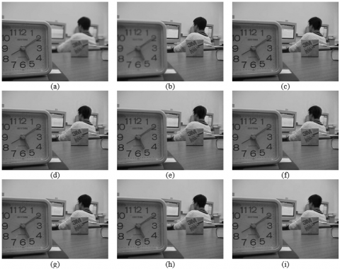
B-1. Multifocus image fusion results of the “Lab” image [42]
B-1. (a) Left-focus source image; (b) Right-focus source image; (c) Reference fusion image; (d) Fusion result of CvT; (e) Fusion result of CvT+PSO; (f) Fusion result of CvT+BAT; (g) Fusion result of LP; (h) Fusion result of LP+PSO; (i) Fusion result of LP+BAT
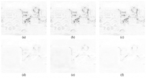
B-2. Differences of the fusion results of "Lab" [42] image with reference fusion image
B-2. (a) Difference of CvT fusion result with reference fusion image; (b) Difference of CvT+PSO fusion result with reference fusion image; (c) Difference of CvT+BAT fusion result with reference fusion image; (d) Difference of LP fusion result with reference fusion image; (e) Difference of LP+PSO fusion result with reference fusion image; (f) Difference of LP+BAT fusion result with reference fusion image
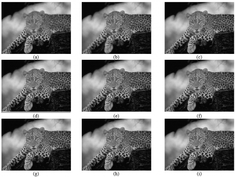
B-3. Multifocus image fusion results of the “Leopard” image [42]
B-3. (a) Left-focus source image; (b) Right-focus source image; (c) Reference fusion image; (d) Fusion result of CvT; (e) Fusion result of CvT+PSO; (f) Fusion result of CvT+BAT; (g) Fusion result of LP; (h) Fusion result of LP+PSO; (i) Fusion result of LP+BAT
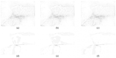
B-4. Differences of the fusion results of "Leopard" [42] image with reference fusion image
B-4. (a) Difference of CvT fusion result with reference fusion image; (b) Difference of CvT+PSO fusion result with reference fusion image; (c) Difference of CvT+BAT fusion result with reference fusion image; (d) Difference of LP fusion result with reference fusion image; (e) Difference of LP+PSO fusion result with reference fusion image; (f) Difference of LP+BAT fusion result with reference fusion image
[1] Arora, J.S. (2004). Introduction to Optimum Design. Elsevier. https://doi.org/10.1016/C2009-0-61700-1
[2] Wang, W., Chang, F. (2011). A multi-focus image fusion method based on laplacian pyramid. JCP, 6(12): 2559-2566. http://dx.doi.org/10.4304/jcp.6.12.2559-2566
[3] Jiang, Q., Jin, X., Lee, S.J., Yao, S. (2017). A novel multi-focus image fusion method based on stationary wavelet transform and local features of fuzzy sets. IEEE Access, 5: 20286-20302. http://dx.doi.org/10.1109/access.2017.2758644
[4] Chien, C.L., Tsai, W.H. (2013). Image fusion with no gamut problem by improved nonlinear IHS transforms for remote sensing. IEEE Transactions on Geoscience and Remote Sensing, 52(1): 651-663. http://dx.doi.org/10.1109/tgrs.2013.2243157
[5] Yang, Y., Wan, W., Huang, S., Yuan, F., Yang, S., Que, Y. (2016). Remote sensing image fusion based on adaptive IHS and multiscale guided filter. IEEE Access, 4: 4573-4582. http://dx.doi.org/10.1109/access.2016.2599403
[6] He, L., Yang, X., Lu, L., Wu, W., Ahmad, A., Jeon, G. (2020). A novel multi-focus image fusion method for improving imaging systems by using cascade-forest model. EURASIP Journal on Image and Video Processing, 2020(1): 5. http://dx.doi.org/10.1186/s13640-020-0494-8
[7] Manchanda, M., Sharma, R. (2017). Multifocus image fusion based on discrete fuzzy transform. 2017 International Conference on Wireless Communications, Signal Processing and Networking (WiSPNET), pp. 775-779. http://dx.doi.org/10.1109/wispnet.2017.8299866
[8] Jing, H., Vladimirova, T. (2014). Novel PCA based pixel-level multi-focus image fusion algorithm. 2014 NASA/ESA Conference on Adaptive Hardware and Systems (AHS), pp. 135-142. http://dx.doi.org/10.1109/AHS.2014.6880169
[9] Liu, Y., Liu, S., Wang, Z. (2015). A general framework for image fusion based on multi-scale transform and sparse representation. Information Fusion, 24: 147-164. http://dx.doi.org/10.1016/j.inffus.2014.09.004
[10] Li, H., Manjunath, B.S., Mitra, S.K. (1995). Multisensor image fusion using the wavelet transform. Graphical Models and Image Processing, 57(3): 235-245. http://dx.doi.org/10.1006/gmip.1995.1022
[11] Kou, L., Zhang, L., Zhang, K., Sun, J., Han, Q., Jin, Z. (2018). A multi-focus image fusion method via region mosaicking on Laplacian pyramids. PloS One, 13(5): e0191085. http://dx.doi.org/10.1371/journal.pone.0191085
[12] Starck, J.L., Candès, E.J., Donoho, D.L. (2002). The curvelet transform for image denoising. IEEE Transactions on Image Processing, 11(6): 670-684. http://dx.doi.org/10.1109/tip.2002.1014998
[13] Do, M.N., Vetterli, M. (2005). The contourlet transform: an efficient directional multiresolution image representation. IEEE Transactions on Image Processing, 14(12): 2091-2106. http://dx.doi.org/10.1109/tip.2005.859376
[14] Nason, G.P., Silverman, B.W. (1995). The stationary wavelet transform and some statistical applications. In Wavelets and Statistics, New York, USA, 281-299. http://dx.doi.org/10.1007/978-1-4612-2544-7_17
[15] Da Cunha, A.L., Zhou, J., Do, M.N. (2006). The nonsubsampled contourlet transform: Theory, design, and applications. IEEE Transactions on Image Processing, 15(10): 3089-3101. http://dx.doi.org/10.1109/tip.2006.877507
[16] Singh, S., Gupta, D., Anand, R.S., Kumar, V. (2015). Nonsubsampled shearlet based CT and MR medical image fusion using biologically inspired spiking neural network. Biomedical Signal Processing and Control, 18: 91-101. http://dx.doi.org/10.1016/j.bspc.2014.11.009
[17] Stathaki, T. (2011). Image Fusion: Algorithms and Applications. Elsevier. https://doi.org/10.1016/B978-0-12-372529-5.X0001-7
[18] Pajares, G., De La Cruz, J.M. (2004). A wavelet-based image fusion tutorial. Pattern Recognition, 37(9): 1855-1872. http://dx.doi.org/10.1016/j.patcog.2004.03.010
[19] Blum, R.S., Liu, Z.E. (2005). Multi-Sensor Image Fusion And Its Applications. CRC Press. http://dx.doi.org/10.1201/9781420026986
[20] Chai, Y., Li, H., Zhang, X. (2012). Multifocus image fusion based on features contrast of multiscale products in nonsubsampled contourlet transform domain. Optik, 123(7): 569-581. https://doi.org/10.1016/j.ijleo.2011.02.034
[21] An, H., Qi, Y., Cheng, Z. (2010). A novel image fusion method based on particle swarm optimization. In Advances in Wireless Networks and Information Systems, Berlin, Heidelberg, 527-535. http://dx.doi.org/10.1007/978-3-642-14350-2_66
[22] Fu, W., Huang, S.G., Li, Z.S., Shen, H., Li, J.S., Wang, P.Y. (2016). The optimal algorithm for multi-source RS image fusion. MethodsX, 3: 87-101. http://dx.doi.org/10.1016/j.mex.2015.12.004
[23] Kanmani, M., Narasimhan, V. (2017). An optimal weighted averaging fusion strategy for thermal and visible images using dual tree discrete wavelet transform and self tunning particle swarm optimization. Multimedia Tools and Applications, 76(20): 20989-21010. http://dx.doi.org/10.1007/s11042-016-4030-x
[24] Daniel, E. (2018). Optimum wavelet-based homomorphic medical image fusion using hybrid genetic–grey wolf optimization algorithm. IEEE Sensors Journal, 18(16): 6804-6811. http://dx.doi.org/10.1109/jsen.2018.2822712
[25] Yang, Y., Zhang, Y., Huang, S., Wu, J. (2019). Multi-focus image fusion via NSST with non-fixed base dictionary learning. International Journal of System Assurance Engineering and Management, 1-7. http://dx.doi.org/10.1007/s13198-019-00887-6
[26] Paramanandham, N., Rajendiran, K. (2018). Multi-focus image fusion using self-resemblance measure. Computers & Electrical Engineering, 71: 13-27. https://doi.org/10.1016/j.compeleceng.2018.07.002.
[27] Abdipour, M., Nooshyar, M. (2016). Multi-focus image fusion using sharpness criteria for visual sensor networks in wavelet domain. Computers & Electrical Engineering, 51: 74-88. https://doi.org/10.1016/j.compeleceng.2016.03.011.
[28] Burt, P., Adelson, E. (1983). The Laplacian pyramid as a compact image code. IEEE Transactions on Communications, 31(4): 532-540. http://dx.doi.org/10.1109/tcom.1983.1095851
[29] Gupta, M.M. (1999). Soft Computing and Intelligent Systems: Theory and Applications. Elsevier. https://doi.org/10.1016/B978-0-12-646490-0.X5000-8
[30] Candes, E.J., Donoho, D.L. (2000). Curvelets: A surprisingly effective nonadaptive representation for objects with edges. Stanford Univ Ca Dept of Statistics.
[31] Candes, E., Demanet, L., Donoho, D., Ying, L. (2006). Fast discrete curvelet transforms. Multiscale Modeling & Simulation, 5(3): 861-899. http://dx.doi.org/10.1007/978-3-642-12538-6_6
[32] Wu, C. (2019). Catenary image enhancement method based on Curvelet transform with adaptive enhancement function. Diagnostyka, 20. http://dx.doi.org/10.29354/diag/109175
[33] Lin, J., Chen, C.L., Tsai, S.F., Yuan, C.Q. (2015). New intelligent particle swarm optimization algorithm for solving economic dispatch with valve-point effects. Journal of Marine Science and Technology, 23(1): 44-53.
[34] Yang, X.S. (2010). A new metaheuristic bat-inspired algorithm. In Nature Inspired Cooperative Strategies for Optimization (NICSO 2010): Berlin, Heidelberg, 65-74. http://dx.doi.org/10.1007/978-3-642-12538-6_6
[35] Zhou, Y., Xie, J., Li, L., Ma, M. (2014). Cloud model bat algorithm. The Scientific World Journal, 2014: 1-11. http://dx.doi.org/10.1155/2014/237102
[36] Yildizdan, G., Baykan, Ö.K. (2020). A novel modified bat algorithm hybridizing by differential evolution algorithm. Expert Systems with Applications, 141: 112949. http://dx.doi.org/10.1016/j.eswa.2019.112949
[37] Deligiannidis, L., Arabnia, H.R. (2015). Security surveillance applications utilizing parallel video-processing techniques in the spatial domain. In Emerging Trends in Image Processing, Computer Vision and Pattern Recognition, pp. 117-130. http://dx.doi.org/10.1016/b978-0-12-802045-6.00008-9
[38] Wei, H., Zhu, Z., Chang, L., Zheng, M., Chen, S., Li, P., Li, Y. (2019). A novel precise decomposition method for infrared and visible image fusion. In 2019 Chinese Control Conference (CCC), pp. 3341-3345. http://dx.doi.org/10.23919/chicc.2019.8865921
[39] Rao, S.S. (2009). Engineering Optimization: Theory and Practice. John Wiley & Sons. http://dx.doi.org/10.1002/9781119454816
[40] Marler, R.T., Arora, J.S. (2010). The weighted sum method for multi-objective optimization: New insights. Structural and Multidisciplinary Optimization, 41(6): 853-862. http://dx.doi.org/10.1007/s00158-009-0460-7
[41] Santé-Riveira, I., Boullón-Magán, M., Crecente-Maseda, R., Miranda-Barrós, D. (2008). Algorithm based on simulated annealing for land-use allocation. Computers & Geosciences, 34(3): 259-268.
[42] https://sites.google.com/view/durgaprasadbavirisetti/datasets, accessed on 1 Jan 2020.
[43] Jagalingam, P., Hegde, A.V. (2015). A review of quality metrics for fused image. Aquatic Procedia, 4(Icwrcoe): 133-142. http://dx.doi.org/10.1016/j.aqpro.2015.02.019
[44] Tsagaris, V., Anastassopoulos, V. (2005). Multispectral image fusion for improved rgb representation based on perceptual attributes. International Journal of Remote Sensing, 26(15): 3241-3254. http://dx.doi.org/10.1080/01431160500127609
[45] Leung, L.W., King, B., Vohora, V. (2001). Comparison of image data fusion techniques using entropy and INI. In 22nd Asian Conference on Remote Sensing, 5: 9.
[46] Wang, Z., Bovik, A.C., Sheikh, H.R., Simoncelli, E.P. (2004). Image quality assessment: From error visibility to structural similarity. IEEE Transactions on Image Processing, 13(4): 600-612. http://dx.doi.org/10.1109/tip.2003.819861
[47] Xydeas, C.A., Petrovic, V. (2000). Objective image fusion performance measure. Electronics Letters, 36(4): 308-309. http://dx.doi.org/10.1049/el:20000267
[48] Petrović, V.S., Xydeas, C.S. (2003). Sensor noise effects on signal-level image fusion performance. Information Fusion, 4(3): 167-183. http://dx.doi.org/10.1016/s1566-2535(03)00035-6
[49] Chaudhuri, S., Kotwal, K. (2013). Hyperspectral Image Fusion. Berlin: Springer. https://doi.org/10.1007/978-1-4614-7470-8
[50] Yang, Y., Tong, S., Huang, S., Lin, P., Fang, Y. (2017). A hybrid method for multi-focus image fusion based on fast discrete curvelet transform. IEEE Access, 5: 14898-14913. http://dx.doi.org/10.1109/access.2017.2698217
[51] Rockinger, O. (1999). Image fusion toolbox for Matlab 5.x. http://www.metapix.de/toolbox.htm