Hesam Akbari | Muhammad Tariq Sadiq* | Malih Payan | Somayeh Saraf Esmaili | Hourieh Baghri | Hamed Bagheri
© 2021 IIETA. This article is published by IIETA and is licensed under the CC BY 4.0 license (http://creativecommons.org/licenses/by/4.0/).
OPEN ACCESS
Late detection of depression is having detrimental consequences including suicide thus there is a serious need for an accurate computer-aided system for early diagnosis of depression. In this research, we suggested a novel strategy for the diagnosis of depression based on several geometric features derived from the Electroencephalography (EEG) signal shape of the second-order differential plot (SODP). First, various geometrical features of normal and depression EEG signals were derived from SODP including standard descriptors, a summation of the angles between consecutive vectors, a summation of distances to coordinate, a summation of the triangle area using three successive points, a summation of the shortest distance from each point relative to the 45-degree line, a summation of the centroids to centroid distance of successive triangles, central tendency measure and summation of successive vector lengths. Second, Binary Particle Swarm Optimization was utilized for the selection of suitable features. At last, the features were fed to support vector machine and k-nearest neighbor (KNN) classifiers for the identification of normal and depressed signals. The performance of the proposed framework was evaluated by the recorded bipolar EEG signals from 22 normal and 22 depressed subjects. The results provide an average classification accuracy of 98.79% with the KNN classifier using city-block distance in a ten-fold cross-validation strategy. The proposed system is accurate and can be used for the early diagnosis of depression. We showed that the proposed geometrical features are better than extracted features in the time, frequency, time-frequency domains as it helps in visual inspection and provide up to 17.56% improvement in classification accuracy in contrast to those features.
electroencephalogram signal, depression, second-order differential plot, geometrical features, EEG classification
1.1 Background
Depression is taken into consideration as one of the common mental disorders worldwide that affect the different aspects of a person life. Its behavioral symptoms appear as restlessness feeling, sadness and distress feeling, low energy and persistent tiredness feeling, sleep disorder, as well as despair and guilty feeling. Growing the extent of the illness and untreated will lead to suicide. Hence detection of depression could be viable to prevent the disease progression and its irreversible consequences. According to the report of the World Health Organization (WHO) in 2017, there are more than 300 million people, who are now living with depression. This situation had an increase of more than 18% between 2005 and 2015 [1]. Although depression is treatable by medication cure and psychotherapy session, there are different reasons in which many people currently suffer from the illness worldwide. These reasons are dealt with lack of awareness, no timely diagnosis, improper detection, high cost of treatment and so on.
Physicians and psychologists can diagnostic the depression disorders by counselling sessions and asking relevant questions from subjects, although it has prone to physician's error and experience. For this reason, medical imaging approach like magnetic response imaging (MRI) and positron emotion tomography (PET) scan used for depression diagnostic.
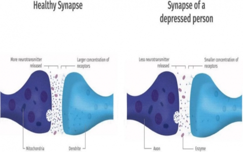
But the main problem of this diagnostic is inaccessibility of these equipment in developing countries, also they are expensive for a large part of society. Besides, PET scan needs to nuclear material which few countries can make it. The activities of the brain in the depression condition became very low in compared to healthy condition. It is due to lesser connection of brain’s synapse in depressed subject in compared to healthy subject. Figure 1 illustrates a schematic comparison of synapses between healthy subjects and depressed patients.
Figure 1. A schematic comparison of synapses tween healthy subjects and depressed patients (adapted from a purchased image from https://www.123rf.com/)
Recently, Electroencephalography (EEG) is considered as a popular tool for detection and investigation of various mental diseases such as Alzheimer [2], dementia [3, 4], epilepsy [5, 6], alcoholism [7-9], attention deficit hyperactivity disorder (ADHD) syndrome [10, 11], autism [12, 13] and motor imagery [14, 15]. The EEG records electrical activity of the brain and depicts the function of brain signals. Since neurons do not properly function in depressed subjects, the synapse has a smaller concentration of receptors and neurotransmitter release is decreased in comparison to healthy subjects. For this reason, depression EEG signals have less complexity (more predictability) compared to standard EEG signals [16, 17]. Visual interpretation and analysing of complex, nonlinear and non-stationary EEG signals by psychiatrist are so difficult, time-consuming and inefficacious procedures. In other word, an automatic method to distinguish normal and depression EEG signals with proper performance is desirable. For that, in this article, we proposed a computer aided detection system based on EEG signals for depression detection.
1.2 Previous works
Therefore, many methods have been proposed to provide an EEG-based diagnosis system for depression subjects in the last two decades. Among those methods, different linear and nonlinear techniques have been used for the identification and detection of depressive disorder.
We have categorized the proposed linear and nonlinear frameworks for depression detection into four groups namely: 1) time method, 2) frequency method, 3) time-frequency method, and 4) deep learning.
The features in the time method have been extracted directly from EEG signals without any processing method. On other hand, features in the frequency method have been extracted from the frequency spectrum of EEG signals. The time method features evaluated the variations of the EEG signal in the time domain and the frequency method evaluated the variation of frequency components of the EEG signals in the frequency domain. In other work, the frequency method measures the variations of the frequency spectrum of the EEG signal. In the following, we reviewed various studies based on time and frequency methods that have been carried out in recent years.
Knott et al. [16] proposed a linear method for the diagnosis of depressive disorder. The authors employed power, frequency, asymmetry, and coherence measures to discriminate between depressed and normal patients which categorizes their framework in time and frequency methods. The results of their research regarding the depressed male patients provide a pattern of aberrant inter-hemispheric synchrony asymmetry and a profile of frontal activation. In a time method, Hosseinifard et al. [18] revealed that the combination of nonlinear features including detrended fluctuation analysis, Higuchi's fractal dimension, correlation dimension, and largest Lyapunov exponent leads to the improvement of k-nearest neighbor (KNN), linear discriminant analysis, and logistic regression classifiers performance and achieved 90% accuracy with logistic regression classifier. Ahmadlou et al. [19] presented a novel nonlinear technique based on the relative convergence of EEGs and named it spatiotemporal analysis of relative convergence. The features were selected by the analysis of variation (ANOVA) statistical test, and then they were considered as inputs for the enhanced probabilistic neural network classifier. This procedure was done for the diagnosis of male and female major depressive disorder patients. We can categorize their work in time methods. Bachmann et al. [20] developed a study based on the time method to compare the spectral asymmetry index technique with Higuchi's fractal dimension method for the diagnosis of depression. They evaluate features using the student’s t-test and achieved good sensitivity (SEN) for the detection of depression. Acharya et al. [21] presented a novel technique using depression diagnosis index with nonlinear features encompassing fractal dimension, the largest Lyapunov exponent, sample entropy, de-trended fluctuation analysis, Hurst’s exponent, higher-order spectra, and recurrence quantification analysis. These features were ranked by the t-value and fed to support vector machine (SVM) classifier, their framework categorizes in time method. This configuration resulted in 98% classification ACC. In another time method, Mumtaz et al. [22] employed synchronization likelihood features as an input to SVM, logistic regression, and naïve Bayesian classifiers and results in 98%, 91.7%, and 93.6% of ACC respectively. Bairy et al. [23] developed a time method by prediction coding method, extracted higher-order statistical features, ranked by receiver operating characteristic (ROC), and reported 94.30% of ACC with bag tree classifier.
The main defect of time method features is that they do not evaluate the EEG signals spectrum which has significant information about the variation of frequency components in the EEG signal. On other hand, the main defect of the frequency method is that it is a significant tool for stationary signals because the frequency components do not change during time. But the EEG signals are non-stationary and their frequency components are not a constant value and change over time. So, extracted parameters by the frequency method cannot be as significant features for the EEG signals as a non-stationary signal.
In a time-frequency method, the EEG signals have been decomposed by wavelet-based techniques and the linear and nonlinear features have been computed from sub-bands.
Extracted features by the time-frequency method can evaluate the variation of EEG signals in both time and frequency domain which is better than the single time method or frequency method. Ahmadlou et al. [17] studied the left and right frontal lobes of major depressive disorder patients by a time-frequency method using the wavelet-chaos methodology proposed by Adeli et al. [24]. Katz's and Higuchi's fractal dimensions features were fed into an enhanced probabilistic neural network for classifying major depressive disorder and normal signals. The reported results showed an accuracy (ACC) of 91.3%. Puthankattil and Joseph [25] suggested an artificial neural network for classifying normal and depressed signals. A discrete wavelet transform as a time-frequency method has been employed to decompose EEG signals; then, relative wavelet energy was calculated for the coefficients of the discrete wavelet transform. They reported a classification ACC of 98.11% for classifying the normal and depressed EEG subjects [25]. In another time-frequency method, Faust et al. [26] extracted entropy features including approximate entropy, sample entropy, renyi entropy, and bispectral phase entropy from wavelet packet decomposition coefficients. Significant features have been selected by the t-test and used as inputs for seven different classifiers. Consequently, the probabilistic neural network classifier provided a classification ACC of 99.5% for detecting healthy and depressed patients. Liao et al. [27] proposed a method called kernel eigen-filter-bank common spatial pattern for feature extraction which resulted in 81.23% classification ACC with SVM classifier. They extracted features from sub-bands of EEG signals which categorizes their method in the time-frequency method. Bachmaan et al. [28] combined linear and nonlinear attributes and achieved 92% ACC with the logistic regression classifier for the detection of depression. Sharma et al. [29] have designed a novel computer-aided diagnosis system that comprised a bandwidth-duration localized and three-channel orthogonal wavelet filter bank (TCOWFB) for the detection of depression subjects. The L2 norm algorithm was utilized as feature extraction from TCOWFB coefficients and resulted in 99.58% ACC in a ten-fold cross-validation strategy by using least square SVM.
In contrast to these three traditional methods for feature extraction, there is a deep learning method. Deep learning is becoming a significant technique in biomedical signal processing applications. But the main defect of deep learning is its cumbersome calculations.
Acharya et al. [30] developed a deep convolutional neural network model for the detection of depression. The experimental results of this work revealed that the classification ACC of 93.5% and 96.0% were attained by the left and right hemispheres, respectively. Their framework categorizes in deep learning.
1.3 Contribution
The main contribution of this study is to utilize the second order difference plot (SODP) of EEG signals, new geometrical features and binary particle swarm optimization (BPSO) as feature selection algorithm in normal and depression EEG signal classification.
With a glance at the past researches, it can be said that most of them have been developed based on wavelet transforms and nonlinear features like entropies. Although these methods can detect depression, but they cannot clearly explain the nonlinear behaviours of normal and depression EEG signals in time domain which can use as a significant parameter for better knowing the nature of depression disorder. For this reason, for the first time we plotted the EEG signals in two dimensional (2D) space by SODP for the classification of depression and normal subjects which is useful method for illustration of dynamic and chaotic nature of the EEG signals.
In other word, we propose a new nonlinear method based on illustration of SODP of EEG signals for the detection of depressed subjects. The SODP is taken into consideration as a technique for 2D illustration of input signal variability [31, 32]. SODP has widely been employed in bio-signals processing applications. SODP has been used for the detection of focal EEG signals [31]. Seizure and seizure-free EEG signals have been classified by extracted features from SODP of EEG signals [32]. SODP was used for human identification in electrocardiography (ECG) signal [33], and it has been used for chronic obstructive pulmonary disease detection through lung sound signal [34]. Due to more stationary morphological behaviors and fewer complexity behaviors of depression EEG signals than normal, this work is focused on applying SODP for 2D illustration of EEG signals. We believe that the pattern of SODP in 2D space can quantify the complexity of EEG signals. These reasons motivated us to use SODP for the classification of normal and depressed EEG signals.
Geometrical features have been extracted from 2D illustration of several bio-signals including hart rate variability (HRV) [35], ECG [36] and EEG [37, 38] for detection of disorders. Geometrical features can quantify the variability and complexity of the 2D shape of bio-signals. Geometrical features have been extracted from Poincaré plot of HRV signals to mortality prediction of ICU cardiovascular patients [39], as well as prediction of epileptic seizures [40], emotions classification [41] and detection of sleep apnea [42]. Geometrical features have been extracted from phase space reconstruction of EEG signals to detection of focal epilepsy [43], seizure [44], ADHD [45] and ECG to heart arrhythmia classification [46]. Geometrical features are significant tool for showing the dynamic of disorders from 2D shape of bio-signals. In this article, geometrical features are extracted from SODP of EEG signals for classification of normal and depressed subjects.
Most of the previous works in biomedical signal processing applications used from statistical approach like ANOVA and student t-test as feature selection tools. In other word, they used from p-values for selecting the significant features; in such a way that features with less than 0.05 p-value can select as significant features. But the approach is not useful when the p-values of all features are less than 0.05; because all features will be used in classifiers whereby the feature vector length will have the highest possible length. We should be noted that the length of the feature vector has a direct relationship to the complexity of the classifier. Thus, a method for founding the shortest feature vector with the best performance is desirable.
In such cases, meta-heuristic algorithms can use for feature selection. In this work, BPSO is applied on extracted geometrical features for selecting the significant features in order to normal and depression EEG signal classification. Concerning the pattern of SODP shape in normal and depressed EEG signals, several nonlinear geometrical features are proposed and BPSO selected the significant features and fed to SVM and KNN classifiers in ten-fold cross validation strategy.
The proposed framework has made innovations in the processing method, feature extraction, and feature selection for depression EEG signals detection based on the previous research. Besides, a new visual method for illustration of the behavior of normal and depression EEG signals have been proposed.
1.4 Organization
The rest of the article is organized as follows. Section 2 describes the used database and gives information about normal and depressed subjects.
Section 3, describes the SODP and bolds the differences between the SODP of normal and depression EEG signals. Section 4 describes the geometrical features and their equations. Section 5 describes the feature selection and classification. Section 6 shows the results. Discussion and conclusion about the results of the proposed framework writes in section 7 and 8, respectively.
Figure 2. A pattern of normal and depressed EEG signals for left and right hemispheres
This study is conducted based on a dataset consisting of 22 healthy (16 men and 6 women) subjects without brain disease and 22 depressed subjects (10 men and 22 women) which candidate to being admitted to the hospital. A committee of senior medical practitioners has authorized the set of data to use for research purposes. This experiment was approved by the Research Ethics Committee of AJA University of Medical Sciences (Approval ID: IR.AJAUMS.REC.1399.049), Tehran, Iran. All the subjects were asked to give written consent. The participants were selected for both groups (depressed and normal situations) in the age group of 23 to 58 years, and then EEG signals were recorded for each participant at the resting state with eyes-open and eyes-closed and consequently, the experiment lasted ten minutes. The recordings were accomplished using bipolar surface electrodes according to the International 10–20 system. During the experiment, the EEG signals were recorded by the FP1-T3 channel from the left hemisphere and FP2-T4 channel from the right hemisphere of the brain. The sampling frequency rate was set to 256 Hz and 50 Hz power line intrusion was eliminated with a notch.
Figure 2 depicts a sample for normal and depressed EEG signals for left and right hemispheres.
Poincaré plot [47] and phase space reconstruction [48, 49] are previously used for 2D illustration of bio-signals. Recently, we used the second-order difference plot (SODP) for the 2D plot of the EEG signal [31]. The SODP can illustrate the complexity of EEG signals in 2D space faster than phase space reconstruction [31]; because of illustration of the phase space matrix requires the calculation of optimum values for delay time τ and embedding dimension d, which they computed from the input signal by using mutual information [50, 51] and false nearest neighbor methods [50], respectively; but in other hand, SODP not needs to computing any parameters. For this reason, this paper is associated with the application of SODP for 2D illustration of the normal and depression EEG signals. SODP illustrates the variability of signals in 2D space. By assuming that EEG signal is EEG(n), then x(n) and y(n) are defined as follows [31, 32]:
$x(n)=E E G(n+1)-E E G(n)$ (1)
$y(n)=E E G(n+2)-E E G(n+1)$ (2)
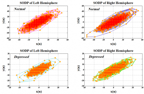
For better understanding the section 2 of present article, we assumed x(n) as $x(n)=\left[x_{1}, x_{2}, \ldots, x_{n-2}\right]$ and y(n) as $y(n)=\left[y_{1}, y_{2}, \ldots, y_{n-2}\right]$. Finally, the SODP is plotted by x(n) versus y(n). Figure 3 illustrates the SODP for the normal and depressed EEG signals.
Figure 3. SODP of normal and depressed EEG signals for the left and right hemispheres
Based on the pattern of the SODP shape of EEG signals, we proposed nonlinear geometrical features for discrimination between normal and depressed subjects. This section is dealt with the description of the proposed geometrical features.
4.1 Standard descriptors (STD)
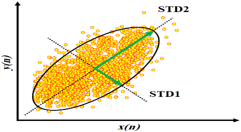
To quantify the Scattering of EEG data on SODP, we used standard descriptors. It is assumed that STD1 and STD2 are two lines with 45 and 135 degrees, respectively. STD1 is introduced as the standard deviation for the projection of SODP on the line perpendicular to the line of identity (y=-x). STD2 is defined as the standard deviation for the projection of SODP on the line of identity (y=x). We can define STD1 and STD2 as following [40]:
$\mathrm{STD} 1=\left(\operatorname{Var}\left((x(n)-y(n)) / 2^{1 / 2}\right)\right)^{1 / 2}$ (3)
$\mathrm{STD} 2=\left(\operatorname{Var}\left((x(n)+y(n)) / 2^{1 / 2}\right)\right)^{1 / 2}$ (4)
where, Var (.) is the variance. In this work, STD=π (STD1×STD2) is utilized to discriminate the features. Figure 4 indicates STD1 and STD2 for SODP.
Figure 4. Illustration of STD of SODP of EEG signal as a used geometrical feature
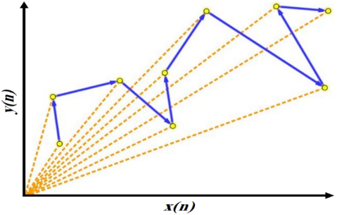
4.2 Summation of the angles between consecutive vectors (SAV)
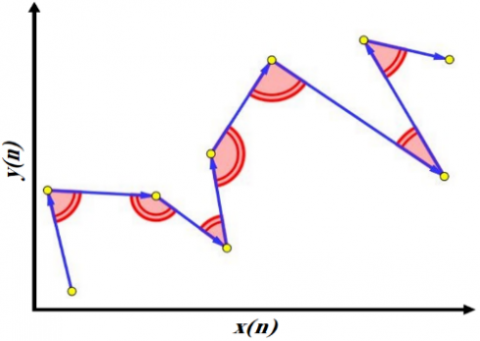
To quantify the behavioral complexity for the EEG signal in the time domain, we computed the angles between consecutive vectors on SODP, which can lead to show better information about changes in the EEG signal over time [39]. Every three points on SODP makes two successive vectors. Assume that $\left(x_{i}, y_{i}\right),\left(x_{i+1}, y_{i+1}\right)$ and $\left(x_{i+2}, y_{i+2}\right)$ are related to coordinates of three successive points, respectively. Then, we can make two successive vectors by using these three points as follow:
$a=\left(x_{i+1}-x_{i}, y_{i+1}-y_{i}\right)=\left(x_{m}, y_{m}\right)$ (5)
$b=\left(x_{i+2}-x_{i+1}, y_{i+2}-y_{i+1}\right)=\left(x_{m+1}, y_{m+1}\right)$ (6)
Thereafter, the angle between two consecutive vectors a and b is defined as follows:
$\cos \theta=\frac{a \cdot b}{|a||b|}=\frac{x_{m} x_{m+1}+y_{m} y_{m+1}}{\sqrt{x_{m}^{2}+y_{m}^{2}}+\sqrt{x_{m+1}^{2}+y_{m+1}^{2}}}$ (7)
where, |a| and |b| denote the length of vectors a and b, respectively. Also, a.b denotes the inner product of vectors a and b. Finally, the summation of the angles between consecutive vectors is calculated as following:
$S A V=\sum_{m=1}^{n-2} \frac{x_{m} x_{m+1}+y_{m} y_{m+1}}{\sqrt{x_{m}^{2}+y_{m}^{2}}+\sqrt{x_{m+1}^{2}+y_{m+1}^{2}}}$ (8)
SAV is the summation of the angles between consecutive vectors. Figure 5 displays the SAV for SODP.
Figure 5. Illustration of SAV of SODP of EEG signal as a used geometrical feature
4.3 Summation of distances to coordinate (SDC)
The distance of data points to coordinate plane for SODP of normal EEG signals are more than depressed signals. This issue mentions that we need to compute the summation of distances of points of SODP to coordinate in normal and depression signals as a feature. It can be calculated as follows [39]:
$S D C=\sum_{i=1}^{n-2} \sqrt{x(i)^{2}+y(i)^{2}}$ (9)
where, x(.) and y(.) indicate ith point coordinate on SODP. Also, SDC is the summation of distances to coordinate. Figure 6 demonstrates the SDC for SODP.
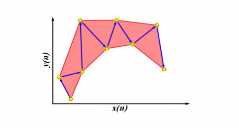
4.4 Summation of the triangle area using three successive points (STA)
As can be observed in Figure 2, SODP of normal EEG signals occupies more area than depressed EEG signals. This issue leads us to compute the area as a geometrical feature. For this reason, we computed the summation of the triangle areas, which can be made by three successive points on SODP as a feature. If $\left(x_{i}, y_{i}\right),\left(x_{i+1}, y_{i+1}\right)$ and $\left(x_{i+2}, y_{i+2}\right)$ are three successive points on SODP, the summation of triangle areas is calculated as following [39]:
$S T A=\frac{1}{2} \sum_{i=1}^{n-2}\left|\operatorname{det}\left[\begin{array}{ccc}x_{i} & x_{i+1} & x_{i+2} \\ y_{i} & y_{i+1} & y_{i+2} \\ 1 & 1 & 1\end{array}\right]\right|$ (10)
where, n denotes the length of x(n) and y(n), STA is the summation of triangle area using three successive points. Figure 7 depicts the STA for SODP.
Figure 6. Illustration of SDC of SODP of EEG signal as a used geometrical feature
Figure 7. Illustration of STA of SODP of EEG signal as a used geometrical feature
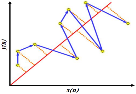
4.5 Summation of the shortest distance from each point relative to the 45-degree line (SSHD)
It can be understood from Figure 2 that the SODP for normal EEG signals is wider than depressed EEG signals. To quantify this element for SODP, we calculate the shortest distance from each point to the 45-degree line as a feature. If $\left(x_{i}, y_{i}\right)$ is a point on SODP, we can calculate the summation of the shortest distance from each point relative to the 45-degree line as [37]:
$S S H D=\sum_{i=1}^{n-2} \frac{|x(i)-y(i)|}{\sqrt{2}}$ (11)
where, n denotes the length of signal x(n) and y(n). Also, SSHD is the summation of the shortest distance from each point relative to the 45-degree line. Figure 8 exhibits the SSHD for SODP.
Figure 8. Illustration of SSHD of SODP of EEG signal as a used geometrical feature
4.6 Summation of the centroid to centroid distance of successive triangles (SCC)
To quantify the self-similarity of the SODP pattern, we computed the summation of distances between the centers of successive triangles as a feature. To achieve this purpose, we should calculate the center of each triangle. We said that every three successive points on SODP make a triangle. To attain the centroid coordinate of each triangle, we should calculate the average coordinates for three successive points, which are edges triangle as follow:
$x_{C}=\frac{x_{i}+x_{i-1}+x_{i-2}}{3}$ (12)
$y_{C}=\frac{y_{i}+y_{i-1}+y_{i-2}}{3}$ (13)
where, $\left(x_{i-2}, y_{i-2}\right),\left(x_{i-1}, y_{i-1}\right)$ and $\left(x_{i}, y_{i}\right)$ are coordinates of triangle edges. Also, $x_{C}$ and $y_{C}$ indicate the coordinate of the centroid of the triangle. Then, by assuming that $\left(x_{C_{i}}, y_{C_{i}}\right)$ and $\left(x_{C_{i+1}}, y_{C_{i+1}}\right)$ are centroid coordinates for two successive triangles, we can compute the summation of centroid to centroid distance for successive triangles as following:
$S C C=\sum \sqrt{\left(x_{C_{i+1}}-x_{C_{i}}\right)^{2}+\left(y_{C_{i+1}}-y_{C_{i}}\right)^{2}}$ (14)
SCC is the summation of centroid to centroid distance for successive triangles. Figure 9 shows the SCC for SODP.
Figure 9. Illustration of SCC of SODP of EEG signal as a used geometrical feature
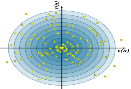
4.7 Central tendency measure (CTM)
Central tendency measure (CTM) is used for quantifying the degree of variability for SODP of EEG signals [31, 32]. If it is assumed that there are N data points on SODP, we can draw a circle with radius r from the coordinate center, which covers M data points of SODP. Afterward, the CTM is defined as the ratio of M/N:
$C T M=\frac{1}{N} \sum_{n=1}^{N} q\left(b_{n}\right)$ (15)
$q\left(b_{n}\right)=\left\{\begin{array}{ccc}1 & \text { if } & \sqrt{[x(n)]^{2}+[y(n)]^{2}} \leq r \\ 0 & & \text { otherwise }\end{array}\right.$ (16)
In this study, we set the range of CTM to 5, 10, 15, …, 90, 95 and computed the corresponding r. Finally, we used $\pi r^{2}$ a feature. In other words, we extracted 19 features to quantify the variability of SODP (i.e. CTM 5, CTM10, CTM15, …, CTM90, CTM95). Figure 10 displays the CTMs for SODP.
Figure 10. Illustration of CTMs of SODP of EEG signal as a used geometrical feature
4.8 Summation of successive vector lengths (SSVL)
Every two successive points on SODP make a vector. To quantify the amplitude changes of EEG signals in the time domain, which can be defined as a covered distance for SODP of EEG signals on a coordinate plane, we calculate the summation of successive vector lengths (SSVL) as a feature. It is defined as following [37]:
$S S V L=\sum_{i=1}^{n-1} \sqrt{\left(x_{i+1}-x_{i}\right)^{2}+\left(y_{i+1}-y_{i}\right)^{2}}$ (17)
where, n denotes the length of x(n) and y(n). Also, $\left(x_{i}, y_{i}\right)$ and $\left(x_{i+1}, y_{i+1}\right)$ indicate the centroid coordinates for two successive points, which make a vector. The SSVL for SODP is shown in Figure 11.
Figure 11. Illustration of SSVL of SODP of EEG signal as a used geometrical feature
A summary of the concept and meaning of proposed geometrical features is given in the Table 1.
Table 1. The geometrical features and their meaning
|
Feature |
Meaning |
|
STD |
Quantifies the scattering of SODP points on the coordinate plane |
|
SAV |
Quantifies the complexity of SODP by measuring the variation of angles |
|
SDC |
Quantifies the scattering of SODP from coordinate center |
|
STA |
Quantifies the area of SODP |
|
SSHD |
Quantifies the scattering of SODP from 45-degree line |
|
SCC |
Quantifies the self-similarity of the SODP shape |
|
CTMs |
Quantifies the variation of SODP shape from coordinate center |
|
SSVL |
Quantifies the variation of length of SODP shape |
The BPSO algorithm is considered as one of the meta-heuristic algorithms for solving the problems with the least information [52]. In many applications, it belongs to the swarm intelligence algorithms and is used as a solution for solving binary optimization problems. In this work, we used BPSO as a feature selection method. The number of particles (N), maximum number of iterations (T), cognitive factor (C1), social factor (C2), maximum velocity (Vmax), maximum bound on inertia weight (Wmax), and minimum bound on inertia weight (Wmin) are the parameters of BPSO algorithm [53]. In this work, for implementation of the BPSO algorithm, the value of N, T, C1, C2, Vmax, Wmax, and Wmin parameters are selected to 10, 100, 2, 2, 6, 0.9, and 0.4, respectively. Besides, the performance of the classifier is used as the fitness function in the BPSO algorithm.
Two famous classifiers namely SVM and KNN are used for the classification of the selected geometrical features by the BPSO algorithm.
The SVM is taken into account as a supervised learning method [54-56]. In recent years, it has shown acceptable performance for classification and solving regression problems. The SVM classifier mapped the training data into a high dimension space by the kernel function. In the new space, a hyper-plane is separated the data into different classes. The selection of kernel function has a direct relationship to the performance of the SVM classifier. In this work, the radial basis function (RBF) is used as the kernel function for mapping of the dataset. Sigma value in RBF is changed from 0.1 to 1.5 by 0.1 steps.
The KNN is characterized as a non-parametric and simple method with simple implementation. KNN algorithm calculates the distance between an input test data and all training samples in a training dataset [29, 57]. Then, K samples are taken from the training dataset, which has the nearest distance to the test data. Then, they are saved as a new dataset. Thus, a class that has the most frequent items in the new set is assigned as the class of test data. There are different metrics for computation of the distance metric such as Euclidean and city block distances. The value of K in the KNN algorithm is an important parameter in the KNN classifier. For this reason, in this work, the value of k is changed from 2 to 9 by one step.
In this paper, we used SODP to plot the variations of EEG signals in 2D space. Figures 2 and 3 show the EEG signals and their SODP for depressed and normal subjects. Aimed at the pattern of SODP for normal and depression EEG signals, we proposed the number of 26 nonlinear geometrical features including STD, SAV, SDC, STA, SSHD, SCC, 19 CTMs (i.e.CTM5, CTM10, …, CTM90, CTM95) and SSVL for classification of normal and depressed subjects.
Table 2 gives the mean, standard deviation and p-value for the extracted features. According to the obtained results, we can understand that the proposed geometrical features within the normal groups considerably have higher mean values than the depressed groups in both hemispheres.
Table 2. Mean ± standard deviation values and p-values of features
|
Left hemisphere |
|||
|
Features |
Normal |
Depression |
p-value |
|
STD |
829±1.01e+4 |
196±4.53e+2 |
1.47E-295 |
|
SAV |
74087±3.71e+3 |
60318±1.42e+4 |
0 |
|
SDC |
38274±1.51e+4 |
19342±1.09e+4 |
0 |
|
STA |
199631±3.07e+6 |
40489±1.22e+5 |
0 |
|
SSHD |
11076±4.82e+3 |
4544±3.55e+3 |
0 |
|
SCC |
34957±1.45e+4 |
14533±1.09e+4 |
0 |
|
CTM5 |
42±1.94e+1 |
11±1.93e+1 |
0 |
|
CTM10 |
88±3.81e+1 |
24±3.98e+1 |
0 |
|
CTM15 |
141±6.07e+1 |
38±6.26e+1 |
0 |
|
CTM20 |
200±8.61e+1 |
54±8.86e+1 |
0 |
|
CTM25 |
269±1.19e+2 |
73±1.18e+2 |
0 |
|
CTM30 |
347±1.48e+2 |
95±1.51e+2 |
0 |
|
CTM35 |
437±1.87e+2 |
120±1.88e+2 |
0 |
|
CTM40 |
541±2.33e+2 |
150±2.31e+2 |
0 |
|
CTM45 |
664±2.89e+2 |
186±2.81e+2 |
0 |
|
CTM50 |
808±3.58e+2 |
228±3.40e+2 |
0 |
|
CTM55 |
979±4.42e+2 |
278±4.10e+2 |
0 |
|
CTM60 |
1187±5.67e+2 |
340±4.96e+2 |
0 |
|
CTM65 |
1448±9.01e+2 |
417±6.05e+2 |
0 |
|
CTM70 |
1800±2.21e+3 |
513±7.41e+2 |
0 |
|
CTM75 |
2311±5.82e+3 |
639±9.22e+2 |
0 |
|
CTM80 |
3040±1.25e+4 |
814±1.18e+3 |
0 |
|
CTM85 |
4084±2.26e+4 |
1086±1.61e+3 |
0 |
|
CTM90 |
5966±4.68e+4 |
1605±2.66e+3 |
0 |
|
CTM95 |
9855±1.02e+5 |
3120±7.41e+3 |
0 |
|
SSVL |
23889±1.05e+4 |
9843±7.63e+3 |
0 |
|
Right hemisphere |
|||
|
Features |
Normal |
Depression |
p-value |
|
STD |
1235± 2.14e+4 |
164±7.55e+2 |
0 |
|
SAV |
75012±3.40e+3 |
59136±1.38e+4 |
0 |
|
SDC |
40837± 2.16e+4 |
18649±9.18e+3 |
0 |
|
STA |
293033±5.58e+6 |
29071±1.86e+5 |
0 |
|
SSHD |
11963±6.60e+3 |
4181±2.63e+3 |
0 |
|
SCC |
37656±1.92e+4 |
13504±7.84e+3 |
0 |
|
CTM5 |
47±1.90e+1 |
10±1.25e+1 |
0 |
|
CTM10 |
98±3.91e+1 |
21±2.49e+1 |
0 |
|
CTM15 |
157±6.10e+1 |
33±3.80e+1 |
0 |
|
CTM20 |
223±8.65e+1 |
47±5.23e+1 |
0 |
|
CTM25 |
299±1.15e+2 |
63±6.87e+1 |
0 |
|
CTM30 |
385±1.48e+2 |
82±8.81e+1 |
0 |
|
CTM35 |
486±1.88e+2 |
104±1.10e+2 |
0 |
|
CTM40 |
602±2.34e+2 |
130±1.36e+2 |
0 |
|
CTM45 |
738±2.89e+2 |
162±1.67e+2 |
0 |
|
CTM50 |
896±3.57e+2 |
199±2.06e+2 |
0 |
|
CTM55 |
1087±4.46e+2 |
244±2.52e+2 |
0 |
|
CTM60 |
1317±5.70e+2 |
299±3.09e+2 |
0 |
|
CTM65 |
1604±8.49e+2 |
367±3.83e+2 |
0 |
|
CTM70 |
1995±2.19e+3 |
454±4.88e+2 |
0 |
|
CTM75 |
2687±1.02e+4 |
568±6.48e+2 |
0 |
|
CTM80 |
3755±2.58e+4 |
728±9.38e+2 |
0 |
|
CTM85 |
5379±5.17e+4 |
974±1.56e+3 |
0 |
|
CTM90 |
8366±1.07e+5 |
1433±3.25e+3 |
0 |
|
CTM95 |
16520±2.92e+5 |
2555±8.14e+3 |
0 |
|
SSVL |
25806±1.43e+4 |
9049±5.66e+3 |
0 |
In other words, SODP of normal EEG signals occupies more areas than the normal subjects (see Figure 3). Another information that we can realize through Figure 3 coincides with the complexity of SODP in EEG signals. According to Figure 3, it is clear that the SODP of normal EEG signals has a more complex shape than depression. On the other hand, the SODP of depression EEG signals has more regular shape than the normal cases. We can say this concept by analysing the standard division values of features in Table 2, because of the standard deviation of features in depression EEG signals are less than normal EEG signals. It may be due to the decreased activity of neurons in the depressed subject’s brain. It has also been found in the previous studies that the depression EEG signals have more stationary behavior and deal with less complexity (more probability) in comparison with the normal EEG signals [29, 30]. Kruskal-Wallis statistical test can show the ability of feature in discrimination of classes in binary classification [6-10]. Kruskal-Wallis statistical test computed the p-value for the extracted features for the normal and depression EEG signals [8, 9]. The lesser p-value indicates that the proposed feature has more ability in discrimination of classes [27, 28]. In this work, the “Kruskal-Wallis” function in MATLAB is used to calculate the p-value for the features. Since the resulted p-values for all extracted features were zero (except the SAV in the left hemisphere with the value of 1.47E-295), so we can argue that all of the proposed geometrical features can be used for detection of depression EEG signals in both hemispheres. Besides BPSO is used as a feature selection technique to reduce the feature vector arrays. In this work, the performance of the SVM classifier with RBF kernel function and KNN classifier with Euclidean and city-block distances in tenfold cross validation strategy are chosen as fitness function in the BPSO algorithm. For the implementation of BPSO in MATLAB, the written function by Too et al. has been used [58]. The selected features by BPSO in the right and left hemispheres with SVM and KNN classifier fitness function are written in Table 3.
These features are fed as input for SVM and KNN classifiers in a ten-fold cross-validation strategy.
In ten-fold cross-validation, the dataset is divided into ten equal subsets. Then, the classifier is tested ten times by one of the subsets and trained by the other subsets (i.e., the nine remaining subsets). In the ten-fold cross-validation strategy, each subset of data is used once as test data and nine times as training data in a classifier. Finally, summation values of true positive (TP), false positive (FP), true negative (TN) and false-negative (FN) from ten times running of the classifier are used for computation of classifier performance. TP, TN, FP and FN parameters are defined as follow:
TP: when a test signal with the depression label is correctly identified by the classifier as a depression signal.
FP: when a test signal with the normal label is incorrectly identified by the classifier as a depression signal.
TN: when a test signal with a normal label is correctly identified by the classifier as a normal signal.
FN: when a test signal with the depression label is incorrectly identified by the classifier as a normal signal.
Thereafter, various objective parameters including: accuracy (ACC), sensitivity (SEN), specificity (SPE), positive predictive value (PPV), negative predictive value (NPV) and Matthews correlation coefficient (MCC) are computed for evaluation of classifier performance. These are determined as follow:
$A C C=\frac{T P+T N}{T P+T N+F P+F N} \times 100$ (18)
$S E N=\frac{T P}{T P+F N} \times 100$ (19)
$S P E=\frac{T N}{T N+F P} \times 100$ (20)
$P P V=\frac{T P}{T P+F P} \times 100$ (21)
$N P V=\frac{T N}{T N+F N} \times 100$ (22)
$M C C=\frac{T P \times T N-F N \times F P}{\sqrt{(T P+F N) \times(T P+F P) \times(T N+F N) \times(T N+F P)}}$ (23)
Table 3. Selected features by BPSO algorithm with SVM and KNN classifiers performance fitness function
|
Selected features |
|
|
Fitness function |
Left hemisphere |
|
SVM (RBF kernel function) |
STD, SAV, SDC, STA, SSHD, SCC,CTM40, CTM60, CTM65, CTM70, CTM85, CTM90, CTM95 |
|
KNN (City-block distance) |
STD, SSHD, SCC, SSVL, CTM5, CTM10, CTM60, CTM65 , CTM70, CTM85, CTM90, CTM95 |
|
KNN (Euclidean distance) |
STD, SSHD, SCC, CTM5, CTM10, CTM30, CTM45 , CTM60, CTM65, CTM85, CTM90, CTM95 |
|
Fitness function |
Right hemisphere |
|
SVM (RBF kernel function) |
STD, SAV, STA CTM5,CTM10,CTM30, CTM45, CTM60, CTM65, CTM70, CTM85, CTM90, CTM95 |
|
KNN (City-block distance) |
SAV, SDC, CTM25, CTM30, CTM35, CTM45, CTM50, CTM65, CTM70, CTM85, CTM90, CTM95 |
|
KNN (Euclidean distance) |
STA, SAV , SCC, SSVL, CTM20, CTM35, CTM40, CTM50 , CTM60, CTM65, CTM75, CTM90, CTM95 |
Table 4. Performance of SVM classifier with RBF kernel function in the classification of geometrical features
|
Objective parameters |
Hemisphere |
|
|
Left |
Right |
|
|
ACC (%) |
96.95 |
98.30 |
|
SEN (%) |
96.09 |
97.53 |
|
SPE (%) |
97.81 |
99.07 |
|
PPV (%) |
97.78 |
99.06 |
|
NPV (%) |
96.16 |
97.57 |
|
MCC |
0.94 |
0.96 |
|
RBF parameter |
0.2 |
0.2 |
Table 5. Performance of KNN classifier with Euclidean distance in the classification of geometrical features
|
Objective parameters |
Hemisphere |
|
|
Left |
Right |
|
|
ACC (%) |
97.79 |
98.58 |
|
SEN (%) |
96.79 |
97.63 |
|
SPE (%) |
98.79 |
99.53 |
|
PPV (%) |
98.77 |
99.53 |
|
NPV (%) |
96.85 |
97.67 |
|
MCC |
0.96 |
0.97 |
|
Number of K |
2 |
2 |
Table 6. Performance of KNN classifier with City block distance in the classification of geometrical features
|
Objective parameters |
Hemisphere |
|
|
Left |
Right |
|
|
ACC (%) |
97.84 |
98.79 |
|
SEN (%) |
96.14 |
97.72 |
|
SPE (%) |
99.53 |
99.86 |
|
PPV (%) |
99.52 |
99.86 |
|
NPV (%) |
96.27 |
97.77 |
|
MCC |
0.96 |
0.98 |
|
Number of K |
4 |
6 |
The results of the tables reveal that the proposed geometrical features provide average classification ACC of 96.95% and 98.30%, SEN of 96.09% and 97.53%, SPE of 97.81% and 99.07% when we used SVM classifier with RBF kernel in the left and right hemispheres, respectively.
Also, average classification ACC of 97.79% and 98.58%, SEN of 96.79% and 97.63%, SPE of 98.79% and 99.53% when we used the KNN classifier with Euclidean distance in the left and right hemispheres, respectively.
In the same way, average classification ACC 97.84% and 98.79%, SEN of 96.14% and 97.72%, SPE of 99.53% and 99.86% when we used KNN classifier with City block distance in the left and right hemispheres, respectively.
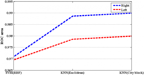
For comparing the capability of used classifiers in classification of normal and depression EEG signals, area under the ROC curve for SVM classifier with RBF kernel function and KNN classifier with Euclidian and City block distances are showed in Figure 12.
Figure 12. The ROC curve for classifiers
It is clearly from Tables 4 to 6 and Figure 12 that the EEG signals of right hemisphere is better than left hemisphere in classification of normal and depression EEG signals. To implement the analysis process, a computer system was employed with the specifications of i5-M480 CPU (2.67 GHz), 6GB RAM, and MATLAB 2014a software package was considered for the purpose. The analysis results indicate a small run time, which is due to the simplicity of the proposed method. Also, our proposed method requires less than 0.02 seconds for the extraction of all 26 geometrical features from an input test signal and less than 0.001 seconds for classification. The proposed method requires less computational time because of applying a minimum number of arrays in the feature vector. The proposed method will require less time when implementing with C++ codes.
In this article, EEG signals of normal and depression groups are plotted by SODP and 26 nonlinear geometrical features are extracted. After that, BPSO selected significant features and fed to SVM and KNN classifiers. Finally objective parameters including ACC, SE, SPE, PPV and MCC calculated for evaluating the geometrical features performance in normal and depression EEG signal classification task. Proposed method evaluated by using EEG signals acquired from 22 normal and 22 depressed subjects. The FP1-T3 and FP2-T4 bipolar channels on the left and right halves of the brain have made all EEG signals. We showed that mean and standard deviation of geometrical features in normal EEG signals are more than depression EEG signal; besides, SODP of depression EEG signals has more rhythmic and regular shape than normal EEG signals which it can may due to increasing connection between the synapses in depressed brain in compared to normal brain. This concept has been reported in previous work in such a way that EEG signals in the depressed group have more stationary morphological behaviors and fewer complexity behaviors than normal groups [29-31]. P-value for all features were zero that indicate to ability of geometrical features in normal and depression EEG signals classification task.
For showing the reliability of proposed method, the objective parameters are reported in tenfold cross-validation strategy. Logic, analysis, sequencing, mathematics, language, facts, computation, facts and training are related to the left hemisphere. In the other hand, creativity, imagination, arts, nonverbal skills, feelings, a tune of songs, daydreaming and creativity are related to the left hemisphere. It is clear that resulted in ACC by EEG signals of the right hemisphere are higher than the left hemisphere in all classifiers. Also, we have found that ACC of KNN classifier with Euclidean and City block distances are better than the SVM classifier with RBF kernel function for both hemispheres. Proposed method resulted to pretty good average classification ACC of 97.84% and 98.79% for the left and right hemispheres, respectively.
We showed that EEG signals acquired from the right hemisphere are significant than left hemisphere in classification of normal and depression EEG signals. Similar concept has been obtained in the previous studies which used from FP1-T3 and FP2-T4 channels from left and right hemispheres for depression diagnostic.
However, we cannot expand this consequence for other studies that used from other electrodes for recording EEG signals. Table 7 compares our proposed method with the existing methods in this area.
The results of Table 7 demonstrate that proposed method provides better classification ACC in comparison with the methods developed by references [16-18, 21-23, 25, 27]. Also, our proposed method generates lesser classification ACC than references [26, 29]. The performance of our proposed method has resulted in a ten-fold cross-validation strategy. Whereas, classification ACC of 99.50% (reported by reference [26]) was reached without considering any cross-validation for solving the problem. In other words, the performance of proposed method is reported in rigorous conditions.
Although the reported classification ACC [29] was higher than proposed method, their method used BDL-TCOWFB as a processing tool, which decomposes EEG signals into three steps, and then they computed Logarithm of L2 norm as a feature from TCOWFB coefficients. On the other hand, our proposed method has very lightweight calculations due to the simplicity of SODP plotting and the extraction of proposed geometrical features. Despite the highest classification ACC in [29], we can argue that our method can be implemented easier than the method represented by reference [29]. Besides, we proposed a novel illustration method for visual inspection of normal and depression EEG signals (see Figure 3). It can be a useable tool for psychologists, psychiatrists, neurologists and the other members of the medical team.
Table 7. Comparison of our proposed method with existing methods for the detection of depression
|
Reference, year |
Used Database |
Cross-validation |
ACC (%) |
|
[16], 2001 |
“70 normal and 23 depressed subjects” |
No |
91.3 |
|
[17], 2012 |
“12 normal and 12 depressed subjects” |
No |
91.30 |
|
[25], 2012 |
“15 normal and 15 depressed subjects” |
No |
98.11 |
|
[18], 2013 |
“45 normal and 45 depressed subjects” |
Leave one out |
90.05 |
|
[26], 2014 |
“15 normal and 15 depressed subjects” |
No |
99.50 |
|
[21], 2015 |
“15 normal and 15 depressed subjects” |
No |
98.00 |
|
[27], 2017 |
“20 normal and 20 depressed subjects” |
Leave one out |
81.23 |
|
[22], 2017 |
“30 normal and 34 depressed subjects” |
Ten fold |
98 |
|
[23], 2017 |
“15 normal and 15 depressed subjects” |
Leave one out |
94.30 |
|
[28], 2018 |
“13 normal and 13 depressed subjects” |
Leave one out |
92 |
|
[30], 2018 |
“15 normal and 15 depressed subjects” |
Ten fold |
95.96 |
|
[29], 2018 |
“15 normal and 15 depressed subjects” |
Ten fold |
99.54 |
|
Present study |
“22 normal and 22 depressed subjects” |
Ten fold |
98.79 |
According into Table 7, we can say that the proposed method provides up to 17.56% classification improvement in comparison with other studies in normal and depression EEG signal classification task.
The advantages of proposed method are written bellow:
- Proposed method is an accurate and robust computer aided system in depression detection which provides perfect average classification ACC of 98.79% and the MCC value of 0.98 which indicates the effectiveness of binary classification.
- We showed that SODP of EEG signals can use as biomarker for analysing the intrinsic behaviours of depression disorder. In other word, we proposed a new illustration method for visual inspection of EEG signals for detecting depression in EEG signals (See Figure 3) for medical team.
- The required time for feature extraction and classification of an input signal was near of 0.02 and 0.01 seconds which indicates to simplify and Lightweight of calculations in proposed method.
- proposed method extracts the features directly from SODP of EEG signal and it does not use from any time-frequency method which wavelet packet decomposition [26], discrete wavelet decomposition [17, 19, 25], Fourier transform [16] and TCOWFB [29] have been used for computation of EEG signals coefficients which makes their method complex than proposed method.
- We used from two channels for classification of normal and depression EEG signals while 7 channels [17], 8 channels [27] and 19 channels [19, 22] have been used for classification of normal and depression EEG signals.
- The objective parameters of classifier reported in tenfold cross-validation strategy which makes proposed method more reliable and efficient while the objective parameters reported without any cross validation methods [16, 17, 21, 25, 26].
- We used from BPSO algorithm for reduction the feature vector arrays. BPSO could redact the feature vector from 26 to 12 and 13 arrays. In other word, BPSO discarded more than 50% of extracted geometrical features while 20 [25], 30 [18], 15 [21] and 100 [22] feature have been used for depression detection.
- The proposed method can implement in MATLAB software, then it can installed on computers in medical clinics and hospitals. It can be used easily by physicians and nurses and does not depend on psychiatrist experience or psychological counseling. Of course, it should be noted that physicians make the final diagnosis, but this system can be advantageous for the physician for an accurate diagnosis of depression.
In this article we proposed 26 different geometric features based on the SODP formation pattern in EEG signals for the identification of normal and depression patients. Through Kruskal–Wallis and BPSO method, substantial features were picked and then fed into KNN and SVM classifiers in ten-fold cross validation strategy. The EEG signals of 22 normal and 22 depression patients have been analyzed for the proposed procedure and results showed that the cumulative accuracy of 97.84% and 98.79% is obtained with the left and right hemispheres respectively. It can also be observed from results that the SODP shape of normal EEG signals was more complex (less predictable) than depression signals. Besides the SODP shape of depression EEG signals was more regular than normal signals, which can be a useful tool for visual inspection of EEG signals in normal or depressed subject’s detection. In future, the proposed method can be used for the identification of different disorders such as epilepsy, sleep apnea and schizophrenia etc.
Hesam Akbari and Muhammad Tariq Sadiq are first co-author and Muhammad Tariq Sadiq and Somayeh Saraf Esmaili are corresponding author of present research. The authors would like to thank Dr. Sedigh Ghofrani (Islamic Azad University, Tehran), Dr. Ali Motie Nasrabadi (Shahed Universit, Tehran) for their valuable comments about our research and Jingwei Too (Universiti Teknikal Malaysia Melaka) for sharing BPSO MATLAB functions. Authors are thankful to “Iranian Army” for supporting this research.
|
World Health Organization SEN |
WHO |
|
magnetic response imaging |
MRI |
|
positron emotion tomography |
PET |
|
attention deficit hyperactivity disorder |
ADHD |
|
accuracy |
ACC |
|
Electroencephalography |
EEG |
|
k-nearest neighbor |
KNN |
|
Electrocardiography |
ECG |
|
hart rate variability |
HRV |
|
three-channel orthogonal wavelet filter bank |
TCOWFB |
|
Accuracy |
ACC |
|
Sensitivity |
SEN |
|
specificity |
SPE |
|
positive predictive value |
PPV |
|
negative predictive value |
NPV |
|
Matthews correlation coefficient |
MCC |
|
support vector machine |
SVM |
|
receiver operating characteristic |
ROC |
|
second order difference plot |
SODP |
|
binary particle swarm optimization |
BPSO |
|
analysis of variation |
ANOVA |
|
Standard descriptors |
STD |
|
Summation of the angles between consecutive vectors |
SAV |
|
Summation of distances to coordinate |
SDC |
|
Summation of the triangle area using three successive points |
STA |
|
Summation of the shortest distance from each point relative to the 45-degree line |
SSHD |
|
Summation of the centroid to centroid distance of successive triangles |
SCC |
|
Central tendency measure |
CTM |
|
Summation of successive vector lengths |
SSVL |
|
true positive |
TP |
|
false positive |
FP |
|
true negative |
TN |
|
false-negative |
FN |
[1] https://www.who.int/news-room/fact-sheets/detail/depression, accessed on 11 March 2020.
[2] Duan, F., Huang, Z., Sun, Z., Zhang, Y., Zhao, Q., Cichocki, A., Solé-Casals, J. (2020). Topological network analysis of early Alzheimer’s disease based on resting-state EEG. IEEE Transactions on Neural Systems and Rehabilitation Engineering, 28(10): 2164-2172. https://doi.org/10.1109/TNSRE.2020.3014951
[3] Henderson, G., Ifeachor, E., Hudson, N., Goh, C., Outram, N., Wimalaratna, S., Vecchio, F. (2006). Development and assessment of methods for detecting dementia using the human electroencephalogram. IEEE Transactions on Biomedical Engineering, 53(8): 1557-1568. https://doi.org/10.1109/TBME.2006.878067
[4] Ieracitano, C., Mammone, N., Hussain, A., Morabito, F.C. (2020). A novel multi-modal machine learning based approach for automatic classification of EEG recordings in dementia. Neural Networks, 123: 176-190. https://doi.org/10.1016/j.neunet.2019.12.006
[5] Akbari, H., Saraf Esmaili, S., Farzollah Zadeh, S. (2020). Detection of seizure EEG signals based on reconstructed phase space of rhythms in EWT domain and genetic algorithm. Signal Processing and Renewable Energy, 4(2): 23-36.
[6] Ghofrani, S., Akbari, H. (2019). Comparing nonlinear features extracted in EEMD for discriminating focal and non-focal EEG signals. In Tenth International Conference on Signal Processing Systems, 11071: 1107106. https://doi.org/10.1117/12.2523445
[7] Sharma, M., Deb, D., Acharya, U.R. (2018). A novel three-band orthogonal wavelet filter bank method for an automated identification of alcoholic EEG signals. Applied Intelligence, 48(5): 1368-1378. https://doi.org/10.1007/s10489-017-1042-9
[8] Shah, S., Sharma, M., Deb, D., Pachori, R.B. (2019). An automated alcoholism detection using orthogonal wavelet filter bank. In Machine Intelligence and Signal Analysis, 473-483. https://doi.org/10.1007/978-981-13-0923-6_41
[9] Sharma, M., Sharma, P., Pachori, R.B., Acharya, U.R. (2018). Dual-tree complex wavelet transform-based features for automated alcoholism identification. International Journal of Fuzzy Systems, 20(4): 1297-1308. https://doi.org/10.1007/s40815-018-0455-x
[10] Karimui, R.Y., Azadi, S., Keshavarzi, P. (2019). The ADHD effect on the high-dimensional phase space trajectories of EEG signals. Chaos, Solitons & Fractals, 121: 39-49. https://doi.org/10.1016/j.chaos.2019.02.004
[11] Karimui, R.Y., Azadi, S., Keshavarzi, P. (2018). The ADHD effect on the actions obtained from the EEG signals. Biocybernetics and Biomedical Engineering, 38(2): 425-437. https://doi.org/10.1016/j.bbe.2018.02.007
[12] Bhat, S., Acharya, U.R., Adeli, H., Bairy, G.M., & Adeli, A. (2014). Autism: Cause factors, early diagnosis and therapies. Reviews in the Neurosciences, 25(6): 841-850. https://doi.org/10.1515/revneuro-2014-0056
[13] Tawhid, M.N.A., Siuly, S., Wang, H. (2020). Diagnosis of autism spectrum disorder from EEG using a time–frequency spectrogram image-based approach. Electronics Letters, 56(25): 1372-1375. https://doi.org/10.1049/el.2020.2646
[14] Sadiq, M.T., Yu, X., Yuan, Z., Aziz, M.Z. (2020). Motor imagery BCI classification based on novel two-dimensional modelling in empirical wavelet transform. Electronics Letters, 56(25): 1367-1369. https://doi.org/10.1049/el.2020.2509
[15] Sadiq, M.T., Yu, X., Yuan, Z., Aziz, M.Z. (2020). Identification of motor and mental imagery EEG in two and multiclass subject-dependent tasks using successive decomposition index. Sensors, 20(18): 5283. https://doi.org/10.3390/s20185283
[16] Knott, V., Mahoney, C., Kennedy, S., Evans, K. (2001). EEG power, frequency, asymmetry and coherence in male depression. Psychiatry Research: Neuroimaging, 106(2): 123-140. https://doi.org/10.1016/S0925-4927(00)00080-9
[17] Ahmadlou, M., Adeli, H., Adeli, A. (2012). Fractality analysis of frontal brain in major depressive disorder. International Journal of Psychophysiology, 85(2): 206-211. https://doi.org/10.1016/j.ijpsycho.2012.05.001
[18] Hosseinifard, B., Moradi, M.H., Rostami, R. (2013). Classifying depression patients and normal subjects using machine learning techniques and nonlinear features from EEG signal. Computer Methods and Programs in Biomedicine, 109(3): 339-345. https://doi.org/10.1016/j.cmpb.2012.10.008
[19] Ahmadlou, M., Adeli, H., Adeli, A. (2013). Spatiotemporal analysis of relative convergence of EEGs reveals differences between brain dynamics of depressive women and men. Clinical EEG and Neuroscience, 44(3): 175-181. https://doi.org/10.1177/1550059413480504
[20] Bachmann, M., Lass, J., Suhhova, A., Hinrikus, H. (2013). Spectral asymmetry and Higuchi’s fractal dimension measures of depression electroencephalogram. Computational and Mathematical Methods in Medicine, 2013. https://doi.org/10.1155/2013/251638
[21] Acharya, U.R., Sudarshan, V.K., Adeli, H., Santhosh, J., Koh, J.E., Puthankatti, S.D., Adeli, A. (2015). A novel depression diagnosis index using nonlinear features in EEG signals. European Neurology, 74(1-2): 79-83. https://doi.org/10.1159/000438457
[22] Mumtaz, W., Ali, S.S.A., Yasin, M.A.M., Malik, A.S. (2018). A machine learning framework involving EEG-based functional connectivity to diagnose major depressive disorder (MDD). Medical & Biological Engineering & Computing, 56(2): 233-246. https://doi.org/10.1007/s11517-017-1685-z
[23] Bairy, G.M., Lih, O.S., Hagiwara, Y., Puthankattil, S.D., Faust, O., Niranjan, U.C., Acharya, U.R. (2017). Automated diagnosis of depression electroencephalograph signals using linear prediction coding and higher order spectra features. Journal of Medical Imaging and Health Informatics, 7(8): 1857-1862. https://doi.org/10.1166/jmihi.2017.2204
[24] Adeli, H., Ghosh-Dastidar, S., Dadmehr, N. (2007). A wavelet-chaos methodology for analysis of EEGs and EEG subbands to detect seizure and epilepsy. IEEE Transactions on Biomedical Engineering, 54(2): 205-211. https://doi.org/10.1109/TBME.2006.886855
[25] Puthankattil, S.D., Joseph, P.K. (2012). Classification of EEG signals in normal and depression conditions by ANN using RWE and signal entropy. Journal of Mechanics in Medicine and biology, 12(4): 1240019. https://doi.org/10.1142/S0219519412400192
[26] Faust, O., Ang, P.C.A., Puthankattil, S.D., Joseph, P.K. (2014). Depression diagnosis support system based on EEG signal entropies. Journal of Mechanics in Medicine and Biology, 14(3): 1450035. https://doi.org/10.1142/S0219519414500353
[27] Liao, S.C., Wu, C.T., Huang, H.C., Cheng, W.T., Liu, Y.H. (2017). Major depression detection from EEG signals using kernel eigen-filter-bank common spatial patterns. Sensors, 17(6): 1385. https://doi.org/10.3390/s17061385
[28] Bachmann, M., Päeske, L., Kalev, K., Aarma, K., Lehtmets, A., Ööpik, P., Hinrikus, H. (2018). Methods for classifying depression in single channel EEG using linear and nonlinear signal analysis. Computer Methods and Programs in Biomedicine, 155: 11-17. https://doi.org/10.1016/j.cmpb.2017.11.023
[29] Sharma, M., Achuth, P.V., Deb, D., Puthankattil, S.D., Acharya, U.R. (2018). An automated diagnosis of depression using three-channel bandwidth-duration localized wavelet filter bank with EEG signals. Cognitive Systems Research, 52: 508-520. https://doi.org/10.1016/j.cogsys.2018.07.010
[30] Acharya, U.R., Oh, S.L., Hagiwara, Y., Tan, J.H., Adeli, H., Subha, D.P. (2018). Automated EEG-based screening of depression using deep convolutional neural network. Computer Methods and Programs in Biomedicine, 161: 103-113. https://doi.org/10.1016/j.cmpb.2018.04.012
[31] Akbari, H., Ghofrani, S. (2019). Fast and accurate classification F and NF EEG by using SODP and EWT. International Journal of Image, Graphics and Signal Processing (IJIGSP), 11(11): 29-35. https://doi.org/10.5815/ijigsp.2019.11.04
[32] Pachori, R.B., Patidar, S. (2014). Epileptic seizure classification in EEG signals using second-order difference plot of intrinsic mode functions. Computer Methods and Programs in Biomedicine, 113(2): 494-502. https://doi.org/10.1016/j.cmpb.2013.11.014
[33] Altan, G., Kutlu, Y., Yeniad, M. (2019). ECG based human identification using second order difference plots. Computer Methods and programs in Biomedicine, 170: 81-93. https://doi.org/10.1016/j.cmpb.2019.01.010
[34] Altan, G., Kutlu, Y., Pekmezci, A.Ö., Nural, S. (2018). Deep learning with 3D-second order difference plot on respiratory sounds. Biomedical Signal Processing and Control, 45: 58-69. https://doi.org/10.1016/j.bspc.2018.05.014
[35] Behbahani, S., Shahram, F. (2020). Electrocardiogram and heart rate variability assessment in patients with common autoimmune diseases: A methodological review. Turk Kardiyol Dern Ars, 48(3): 312-327. https://doi.org/10.5543/tkda.2019.21112
[36] Nejadgholi, I., Moradi, M.H., Abdolali, F. (2011). Using phase space reconstruction for patient independent heartbeat classification in comparison with some benchmark methods. Computers in Biology and Medicine, 41(6): 411-419. https://doi.org/10.1016/j.compbiomed.2011.04.003
[37] Akbari, H., Esmaili, S. (2020). A novel geometrical method for discrimination of normal, interictal and ictal EEG signals. Traitement du Signal, 37(1): 59-68. https://doi.org/10.18280/ts.370108
[38] Azizi, A., Moridani, M.K., Saeedi, A. (2019). A novel geometrical method for depression diagnosis based on EEG signals. In 2019 IEEE 4th Conference on Technology in Electrical and Computer Engineering.
[39] Moridani, M.K., Setarehdan, S.K., Nasrabadi, A.M., Hajinasrollah, E. (2018). A novel approach to mortality prediction of ICU cardiovascular patient based on fuzzy logic method. Biomedical Signal Processing and Control, 45: 160-173. https://doi.org/10.1016/j.bspc.2018.05.019
[40] Behbahani, S., Dabanloo, N.J., Nasrabadi, A.M., Dourado, A. (2016). Prediction of epileptic seizures based on heart rate variability. Technology and Health Care, 24(6): 795-810. https://doi.org/10.3233/THC-161225
[41] Moharreri, S., Dabanloo, N.J., Maghooli, K. (2019). Detection of emotions induced by colors in compare of two nonlinear mapping of heart rate variability signal: triangle and parabolic phase space (TPSM, PPSM). Journal of Medical and Biological Engineering, 39(5): 665-681. https://doi.org/10.1007/s40846-018-0458-y
[42] Jafari, A. (2013). Sleep apnoea detection from ECG using features extracted from reconstructed phase space and frequency domain. Biomedical Signal Processing and Control, 8(6): 551-558. https://doi.org/10.1016/j.bspc.2013.05.007
[43] Bhattacharyya, A., Sharma, M., Pachori, R.B., Sircar, P., Acharya, U.R. (2018). A novel approach for automated detection of focal EEG signals using empirical wavelet transform. Neural Computing and Applications, 29(8): 47-57. https://doi.org/10.1007/s00521-016-2646-4
[44] Sharma, R., Pachori, R.B. (2015). Classification of epileptic seizures in EEG signals based on phase space representation of intrinsic mode functions. Expert Systems with Applications, 42(3): 1106-1117. https://doi.org/10.1016/j.eswa.2014.08.030
[45] Kaur, S., Singh, S., Arun, P., Kaur, D., Bajaj, M. (2020). Phase space reconstruction of EEG signals for classification of ADHD and control adults. Clinical EEG and Neuroscience, 51(2): 102-113. https://doi.org/10.1177/1550059419876525
[46] Li, Y., Tang, X., Xu, Z., Yan, H. (2018). A novel approach to phase space reconstruction of single lead ECG for QRS complex detection. Biomedical Signal Processing and Control, 39: 405-415. https://doi.org/10.1016/j.bspc.2017.06.007
[47] Goshvarpour, A., Goshvarpour, A. (2020). Diagnosis of epileptic EEG using a lagged Poincare plot in combination with the autocorrelation. Signal, Image and Video Processing, 1-9. https://doi.org/10.1007%2Fs11760-020-01672-w
[48] Boubchir, L. (2020). Editorial commentary on special issue of advances in EEG signal processing and machine learning for epileptic seizure detection and prediction. The Journal of Biomedical Research, 34(3): 149-150. https://doi.org/10.7555/JBR.34.20200700
[49] Soroush, M.Z., Maghooli, K., Setarehdan, S.K., Nasrabadi, A.M. (2020). Emotion recognition using EEG phase space dynamics and POINCARE intersections. Biomedical Signal Processing and Control, 59: 101918. https://doi.org/10.1016/j.bspc.2020.101918
[50] Kantz, H., Schreiber, T. (2004). Nonlinear Time Series Analysis (Vol. 7). Cambridge University Press.
[51] Roulston, M.S. (1999). Estimating the errors on measured entropy and mutual information. Physica D: Nonlinear Phenomena, 125(3-4): 285-294. https://doi.org/10.1016/S0167-2789(98)00269-3
[52] Too, J., Abdullah, A.R., Mohd Saad, N., Tee, W. (2019). EMG feature selection and classification using a Pbest-guide binary particle swarm optimization. Computation, 7(1): 12. https://doi.org/10.3390/computation7010012
[53] Too, J., Abdullah, A.R., Mohd Saad, N. (2019). Binary competitive swarm optimizer approaches for feature selection. Computation, 7(2): 31. https://doi.org/10.3390/computation7020031
[54] Sadiq, M.T., Yu, X., Yuan, Z. (2020). Exploiting dimensionality reduction and neural network techniques for the development of expert brain–computer interfaces. Expert Systems with Applications, 164: 114031. https://doi.org/10.1016/j.eswa.2020.114031
[55] Sadiq, M.T., Yu, X., Yuan, Z., Fan, Z., Rehman, A.U., Li, G., Xiao, G. (2019). Motor imagery EEG signals classification based on mode amplitude and frequency components using empirical wavelet transform. IEEE Access, 7: 127678-127692. https://doi.org/10.1109/ACCESS.2019.2939623
[56] Sadiq, M.T., Yu, X., Yuan, Z., Fan, Z., Rehman, A.U., Ullah, I., Xiao, G. (2019). Motor imagery EEG signals decoding by multivariate empirical wavelet transform-based framework for robust brain–computer interfaces. IEEE Access, 7: 171431-171451. https://doi.org/10.1109/ACCESS.2019.2956018
[57] Moharreri, S., Dabanloo, N.J., Maghooli, K. (2018). Modeling the 2D space of emotions based on the poincare plot of heart rate variability signal. Biocybernetics and Biomedical Engineering, 38(4): 794-809. https://doi.org/10.1016/j.bbe.2018.07.001
[58] Too, J., Abdullah, A. R., Mohd Saad, N., Mohd Ali, N. (2018). Feature selection based on binary tree growth algorithm for the classification of myoelectric signals. Machines, 6(4): 65. https://doi.org/10.3390/machines6040065