Zülfikar Aslan* | Mehmet Akin
© 2020 IIETA. This article is published by IIETA and is licensed under the CC BY 4.0 license (http://creativecommons.org/licenses/by/4.0/).
OPEN ACCESS
This study presents a method that aims to automatically diagnose Schizophrenia (SZ) patients by using EEG recordings. Unlike many literature studies, the proposed method does not manually extract features from EEG recordings, instead it transforms the raw EEG into 2D by using Short-time Fourier Transform (STFT) in order to have a useful representation of frequency-time features. This work is the first in the relevant literature in using 2D time-frequency features for the purpose of automatic diagnosis of SZ patients. In order to extract most useful features out of all present in the 2D space and classify samples with high accuracy, a state-of-art Convolutional Neural Network architecture, namely VGG-16, is trained. The experimental results show that the method presented in the paper is successful in the task of classifying SZ patients and healthy controls with a classification accuracy of 95% and 97% in two datasets of different age groups. With this performance, the proposed method outperforms most of the literature methods. The experiments of the study also reveal that there is a relationship between frequency components of an EEG recording and the SZ disease. Moreover, Grad-CAM images presented in the paper clearly show that mid-level frequency components matter more while discriminating a SZ patient from a healthy control.
schizophrenia, CNN, deep learning, spectrogram
Schizophrenia (SZ) is a serious neuropsychiatric disease that is estimated to affect nearly 1% of the world population. Patients of this disease suffer from hallucinations and delusions as well as diminishment in motivation and difficulty in expressing emotions [1]. These symptoms generally begin in early ages and the damage in the brain caused by the disease increases in time. Early diagnosis of the disease and patient specific treatment may help reduce deformations in the brain, it is, however, difficult even for the experts to diagnose the disease in the early stages [2]. Therefore, development of computer methods to diagnose the disease in order to help clinicians in the decision making has been an important research topic in the relevant literature. Even though most literature methods such as [3, 4] often utilized traditional Machine Learning (ML) algorithms, recent developments in the Deep Learning (DL) make a promising newer direction for the researchers of the field.
Electroencephalography (EEG) recording is an important tool to analyze brain activity and functions. An EEG record contains information obtained from electrical signals detected by use of electrodes placed on different areas of the patient’s head. These signals are often digitized and analyzed by use of dedicated computer programs in order to help experts evaluate the information which is otherwise hard to analyze specifically in the cases like SZ where the raw signal does not directly show any disease related anomaly. In the computer-aided diagnosis (CAD) of SZ, using EEG recordings is not the only way in the literature. In order to perform automatic detection of the disease, researchers used several different medical imaging techniques like magnetic resonance imaging (MRI), positron emission tomography (PET), functional magnetic resonance imaging (fMRI) and diffusion tensor magnetic resonance imaging (DTI). These alternative techniques, however, have not considered as favorable as EEG due to the reasons such as high cost of imaging hardware and images produced by these machines not always being of the desired quality [5]. Therefore, EEG comes into prominence as a low cost and reliable alternative to be used as an input to a CAD system designed to automatically detect many diseases such as SZ [6].
Therefore, in the relevant literature, most of the CAD systems to detect SZ focused on using EEG signals. A great deal of researchers attempted to diagnose the disease by using traditional ML techniques over features extracted from EEG signals. The key to successful diagnosis of the disease is extracting relevant features from the signals and therefore there have been various methods proposed in the literature to this end. In the study of Kim et al. [7], 5 frequency bands from 21-channel EEG recordings are selected. They applied Fast Fourier Transform (FFT) over these bands and spectral power of these bands are calculated by using EEGLAB software [8]. They classified healthy and SZ patients with an accuracy of 62.2% by using the delta frequency. In another study, Dvey-Aharon et al. [9] preprocessed EEG signals by using The Stockwell transformation to extract features [10]. Their method called “TFFO” (Time-Frequency transformation followed by Feature-Optimization) showed a satisfactory accuracy between 92% and 93.9%. Moreover, Johannesen et al. [11] used Support Vector Machines (SVM) to extract most relevant features [12] from the EEG recordings in order to predict working memory performance of healthy and SZ patients. Their method reached an accuracy of 87% in the prediction performance. Similarly, Santos-Mayo et al. [13] tested various ML approaches and feature selection algorithms including electrode grouping and filtering. As a result, they reported Multi-Layer Perceptron (MLP) and SVM algorithms have the best accuracy in classification performance with 93.42% and 92.23%, respectively. Moreover, classification over features obtained from J5 feature selection algorithm [14] performed better. In the study of Aslan and Akın [15], features are extracted from the EEG signals by using Relative Wavelet Energy. These features are then fed to K-Nearest Neighbors algorithm in order to classify healthy and SZ cases. They reported to have reached nearly 90% accuracy performance. Thilakvathi et al. [16] used Support Vector Machines (SVM) algorithm to discriminate SZ patients. They used Hannon Entropy, Spectral Entropy, Information Entropy, Higuchi’s Fractal Dimension and Kolmogorov Complexity values as features used as inputs to SVM. They reported an accuracy of 88.5%. In all these literature methods mentioned up to now, the EEG recordings are not used in raw, instead researchers crafted some features out of EEG signals and fed a ML algorithm of the choice with these features. This feature engineering approach has several advantages like good predictive performance but it requires experts with comprehensive knowledge of the target domain. Also, all these extracted features are ad hoc solutions specific to the data and they are not proven to generalize well with all cases.
As an alternative approach, researchers have recently been investigating Deep Learning (DL) algorithms such as CNN to automatically diagnose SZ patients because DL algorithms do not require the practitioner extract any features manually from the input. The features in the given input are extracted automatically in layers of the network such as convolutional and pooling layers. There are only few literature methods that utilize CNNs to detect SZ in given EEG signals. In one study, Phang et al. [17] proposed a method that accepts brain functional connectivity information as features. These features are extracted from EEG recordings by use of vector autoregressive (VAR) model, partial directed coherence (PDC) and complex network measures of network topology. The obtained features are subsequently fed to two Convolutional Neural Network (CNN) models which in turn are fused into a Fully-Connected Neural Network (FCN) that is capable of classifying healthy controls and SZ patients. They reported an accuracy of 93.06% in the classification task. Their method is reported to reach a satisfactory accuracy but relies on additional data such as brain connectivity features. In another study, Oh et al. [6] utilized a CNN model to classify 19-channel EEG recordings of 14 healthy controls and 14 SZ patients. Their CNN model had a total of 11 layers including regular convolutional, pooling and dense layers. No preprocessing is used and the raw EEG channels are fed into the CNN model all at once. Their method is reported to reach an accuracy of 81.26% for subject based testing and 98.07% for non-subject based testing. Both methods that utilize DL to diagnose SZ lack interpretability due to the use of CNNs as a black-box solution. This is partly because of the fact that raw EEG signals are not obviously correlated with possible visual outcomes of convolution operations.
In this study, we propose a method that attempts to detect SZ patients with high accuracy, simple pipeline and as well as interpretable outputs. The proposed study is novel in the way that it hypothesizes that frequency-time features of an EEG recording is sufficient to automatically discriminate SZ patients. The frequency-time features are obtained by converting raw EEG signals into 2D spectrogram images by using Short-time Fourier Transformation (STFT). As to our knowledge, it is the first time in the relevant literature, spectrograms are used as inputs to detect SZ patients. The most useful features that are thought to be present in these images are automatically extracted by a state-of-art CNN model which also classifies samples into healthy or diseased in later layers of the network. Therefore, the proposed method is advantageous to many literature methods that require expert knowledge to extract useful features from EEG recordings because it extracts features automatically through layers of the CNN. Moreover, when it is contrasted to literature methods that use a CNN, it still has advantages such as interpretable outputs, simpler pipeline and easier to implement architecture. The proposed method is tested against two different datasets each of which contains patients and healthy controls of different age groups. The fact that the proposed method reaches high accuracy (95% and 97%) in both children and adult data show that it is a robust method for the task of automatically diagnosing the SZ disease. Moreover, the obtained accuracy values are better than those of most of the literature methods. It should also be noted that one more advantage of the method is that because it uses images as inputs, the model can output interpretable results such as Grad-CAM images that reveal the relationship between frequency components and the disease.
2.1 Methods
2.1.1 Deep learning
Deep Learning is a recent approach in Machine Learning that adopts hierarchical learning of features with deeper neural network architectures. Network structures in DL looks similar to those utilized in traditional ML, however, they differ in the way that DL algorithms attempt to learn features by themselves automatically while ML methods often require proper features given to the network by the practitioner. DL started to come forward as a successful alternative to traditional ML algorithms only after large-scale datasets become publicly available and the hardware required to process such kind of data become cheaper and thus more accessible. Therefore, recently DL has been frequently used as a method to process, analyze and evaluate medical images mostly in the form of CNNs [18]. This study also uses a CNN model to classify spectrogram images
2.1.2 Convolutional Neural Networks
Convolutional Neural Networks are DL networks that are designed to process multimedia data types (e.g., images) in a way that features can be automatically extracted in a hierarchical manner through the layers of the network [19]. At the core, a CNN model often consists of two modules, a) Feature extraction through convolutional and pooling layers b) Classification stage via Fully-Connected Network layers (FCN) which operates similarly to a traditional Multi-Layer Perceptron (MLP).
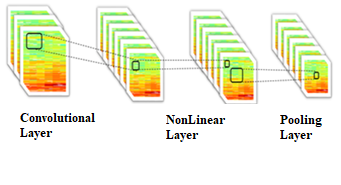
In a regular CNN model, there are a number of subsequent convolutional and pooling layers each of which is responsible to extract features from the previous layer’s output. In this way, early layers of the network extract simple features such as lines in an image and feed later layers with these features so that subsequent layers can process these simple features and extract more complex features like objects in an image. This kind of hierarchical learning of features is inspired from human cortex in which cells respond to visual elements in a similar hierarchical way [20]. Figure 1 depicts a block of convolutional layer, non-linear layer and pooling layer.
Figure 1. A block of convolutional layer, non-linear layer and pooling layer
In a convolutional layer, there are typically many filters, W = W1, W2...., Wk, each of which is used to convolve the input image with a filter to calculate a feature map Xk of the image. Therefore, we have as many feature maps as the number of filters in the convolutional layer. More formally, each feature map is calculated via Eq. (1) where b denotes bias and σ (·) is a non-linear transfer function [21]:
$X_{k}^{l}=\sigma\left(W_{k}^{l-1} * X^{l-1}+b_{k}^{l-1}\right)$ (1)
A convolutional layer is generally followed by a pooling layer in which feature maps are downsampled in accordance with the selected pooling function, max, min or avg. The function of choice is applied to every group of pixels in the feature map and result of the function (e.g., maximum value in that group) is selected to represent the group in the new downsampled feature map. In an overview, a CNN model consists of three different layer types: (1) convolutional layers, (2) pooling layers and (3) a FCN [22].
Convolutional layer is the first layer that extracts features from the input image. The convolution operation uses small matrices (e.g., size 3x3) called filters to learn image features while keeping spatial information in the image. Pooling layer is in general used to reduce the number of parameters. Since it keeps the spatial information, it is often known as a downsampling operation. The behaviour of downsampling operation depends on the function selected. For instance, in max pooling, maximum value in the region of interest is selected to replace all values in that region. The other types, min pooling and avg pooling, do a similar job but they get the minimum or the average value instead. The output of pooling layer is connected to a FCN that does the classification [23]. A FCN is often a MLP with a Softmax output layer. As usual, it is trained with the backpropagation algorithm [24].
2.1.3 VGG-16 architecture
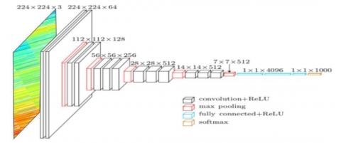
VGG-16 is a state-of-art 16-layer CNN model developed by the Oxford University Visual Geometry Group for the ILSVRC-2014 competition. Its major difference is that it has a deeper architecture than its predecessors. In VGG-16, images are converted to 224x224x3 (RGB) and passed through 5 blocks of convolutional layers each of which has a filter size of 3x3. Each block ends with a max pooling layer in which inputs are downsampled by a factor of 2. Then the acquired feature set is connected to a FCN that completes the classification task. Figure 2 depicts general overview of the VGG-16 architecture [25].
VGG-16 is an example of family of state-of-art CNN models that include other well-known architectures such as CIFAR, Google LeNet and AlexNet. Before choosing VGG-16, we empirically tested other CNN models with other data and observed that with some exceptions all models performed comparably. VGG-16, however, outperformed the others slightly. Therefore, for the sake of simplicity we only show the results with VGG-16 in the paper.
2.1.4 Generating spectrogram images from EEG signals
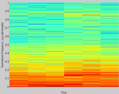
Short-Time Fourier Transformation (STFT) is a general purpose tool that converts a signal in time domain into frequency domain. STFT conversion is calculated by multiplying the transfer function with a window function. Spectrogram is a visual depiction of the signal in the frequency domain within a time interval [26]. Therefore, it shows how the frequency components of the signal change in time. In this study, short segments of the EEG signal (e.g., 5 seconds long) is converted into a spectrogram in order that we can have frequency components of different time points in one image. We used MATLAB software to obtain spectrogram images of these short EEG segments. In the default configuration of MATLAB’s spectrogram function, it generates Nx=1024 samples of a signal that consists of a sum of sinusoids. The normalized frequencies of the sinusoids are 2π/5 rad/sample and 4π/5 rad/sample.
In the example spectrogram in Figure 3, y-axis represents frequency which is normalized between 0 and 1 while x-axis stands for time. Colors approaching red show high values in that frequency whereas colors close to blue are used to show low intensity values. Therefore, in the example spectrogram, it is observed that low frequency components in the signal are more intense than high frequency components at most of the time segments. High frequency components emerge at high values only at few time values and thus mostly depicted with different tones of blue color in the example spectrogram.
2.1.5 General architecture of the proposed method
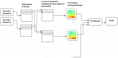
As mentioned our method does not include any manual processing or ad hoc altering of input. Each input, i.e., a set of EEG channel data, is passed through a series of transformations (segmentation, spectrogram generation and CNN evaluation) and finally results in a class value, either SZ patient or a healthy control. Figure 4 depicts general overview of the process.
Figure 2. VGG-16 architecture
Figure 3. An example spectrogram generated by Matlab software
Figure 4. Flowchart of the proposed method
3.1 Material
3.1.1 Dataset A
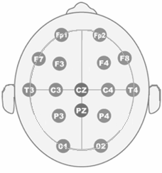
The first dataset used in this study is the set of EEG recordings that belong to 39 healthy control subjects and 45 children that have the same kind of schizophrenic disorder. All SZ patients in this dataset are approved by the Mental Health Research Center (MHRC) experts. None of the patients in this dataset has undergone chemical treatment. The eldest of the SZ patients is 14 years old and the youngest one is 10 years and 8 months old while the eldest and the youngest control subject are 13 years 9 months old and 11 years old, respectively. The average age in both groups is 12 years and 3 months [27]. The data is recorded while the subjects are comfortable, awake, their eyes being shut and 16 electrodes are connected to their head. EEG is recorded in accordance with the international 10-20 standard with the electrode sequence of O1, O2, P3, P4, Pz, T5, T6, C3, C4, Cz, T3, T4, F3, F4, F7 and F8 (See Figure 5). Each EEG recording is 60 seconds long and recorded with a sampling rate of 128 Hz. Therefore, an EEG data for each subject is represented with a 7680 x 16 matrix.
3.1.2 Dataset B
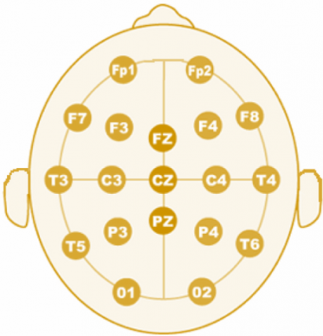
The second dataset utilized in this study contains EEG recordings of 14 healthy controls and 14 SZ patients. This data is recorded by the Institute of Psychiatry and Neurology in Warsaw, Poland from 14 male and 14 female subjects with the average ages of 27.3±3.3 ve 28.3±4.1, respectively. The subjects keep their eyes shut during the recording that is taken with a sampling frequency of 250 Hz for about 12 and 15 minutes. Each record has 19 channels with the electrode sequence of Fp1, Fp2, F7, F3, Fz, F4, F8, T3, C3, Cz, C4, T4, T5, P3, Pz, P4, T6, O1 and O2 (See Figure 6) [28].
Figure 5. 16 channel electrode setup for Dataset A
Figure 6. 19 channel electrode setup for Dataset B
3.2 Experiments
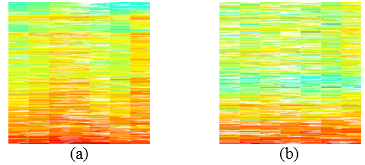
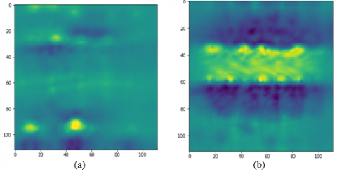
In this study, the proposed method is evaluated against two datasets of samples. In the first dataset (A), there are 16-channel EEG recordings of 39 healthy children and 45 children with SZ disease. Each sample is divided into 5-seconds long segments each of which is represented with a vector of length 10240 (128 values per second x 16 channels x 5 seconds). These vectors are then converted into spectrograms of size 224x224. Therefore, we have 1008 images for 84 individuals in Dataset A. Figure 7 and 8 show example spectrogram images for a healthy control and a SZ patient for Dataset A and B, respectively.
Figure 7. Example spectrogram images from Dataset A for (a) healthy control and (b) SZ patient
Figure 8. Example spectrogram images from Dataset B for (a) healthy control and (b) SZ patient
(a)
(b)
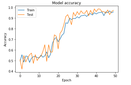
Figure 9. Accuracy against training time in epochs for (a) Dataset A and (b) Dataset B
The data set of spectrogram images is split into train and test sets with a ratio of 80% and 20%, respectively. These images are fed into VGG-16 CNN model in order to classify each as either healthy or SZ patient. The hyper parameters for the network are taken as follows: input image size 112x112, batch-size 128, 1.0e-4 learning rate and optimizer Adam [29]. Through the experiments we observed that 50 epochs of training sufficed in order to reach a convergence of the network. On average, the network reached an accuracy of 95% for the test set.
In the second dataset, there are 19-channel EEG recordings of 28 adults (14 controls and 14 SZ patients). The length of the recordings varied between 12 and 15 minutes. Therefore, in healthy and SZ groups, the length of the recording is set to length of the shortest record in the group. Subsequently, we obtained 173 segments for each healthy control and 148 segments for each SZ patient where length of each segment was again 5 seconds. After this point, a total of 4494 spectrogram images are processed similarly to the ones in Dataset A with the same settings and hyper parameters. As a result, the network reached an accuracy of 97.4% at 30 epochs. Figure 9 shows the change in the accuracy with respect to training time in epochs.
As can be seen in Figure 9, sufficient amount of training is important and affects the accuracy of the model significantly. Unfortunately, there is no predefined number for the required amount of training in the literature and it is in general determined empirically for each dataset through the experiments.
3.3 Evaluation metrics
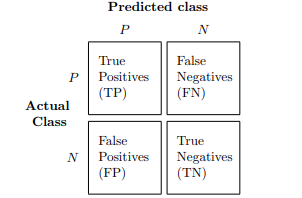
3.3.1 Confusion matrix (as shown in Figure 10 above)
Figure 10. The confusion matrix
The experiments of the study are evaluated and results are confirmed with a number of well-known and widely-used evaluated metrics. The details and interpretations of these metrics are explained in other papers [30, 31] and therefore we only include basic calculations of these metrics.
3.3.2 Prediction error and accuracy
$E R R=\frac{F P+F N}{F P+F N+T P+T N}=1-A C C$ (2)
$A C C=\frac{T P+T N}{E P+F N+T P+T N}=1-E R R$ (3)
3.3.3 False and true positive rates
$F P R=\frac{F N}{N}=\frac{F P}{F P+T N}$ (4)
$T P R=\frac{T P}{P}=\frac{T P}{F N+T P}$ (5)
3.3.4 Precision, recall, F1 score
F1-Score is a more capable metric that can evaluate performance of a classifier in all aspects in a more balanced way than a single FPR or TPR metric. In order to calculate, F1-Score, Precision (PRE), also known as TPR or Sensitivity (SEN), and Recall metrics should be calculated beforehand. Eqns. (6)-(8) show the calculation of F1-score [31].
$P R E=\frac{T P}{T P+F P}$ (6)
$R E C=T P R=\frac{T P}{P}=\frac{T P}{F N+T P}$ (7)
$F_{1}=2 \cdot \frac{P R E \cdot R E C}{P R E+R E C}$ (8)
As an additional widely-used metric, the Specificity (SPC) measures how well is the classifier in avoiding misclassifications and is ideally equal to 1.
$S P C=T N R=\frac{T N}{N}=\frac{T N}{F P+T N}$ (9)
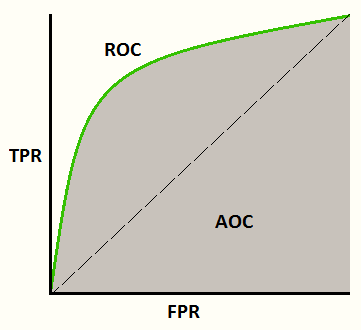
3.3.5 Receiver operator characteristic (ROC) and AUC (area under the curve)
Figure 11. An example ROC curve
The ROC curve is a graphical common metric used in the ML literature. It plots TPR (y-axis) against FPR (x-axis) values changing with respect to different threshold values used by the binary-classifier while discriminating between 0 and 1 values. The AUC (or AOC - Area of the Curve) value is the total area occupied under the curve. It is better when the AUC value is high because a high AUC tells that the classifier does well with most threshold values while classifying “0” s as “0” and “1” s as “1”. Figure 11 shows an example ROC curve.
An ideal classifier should detect diseased patients with a high rate while ruling out all healthy controls as non-diseased. Therefore, both Precision and Recall metrics of the classifier should be high at the same time which eventually results in a high F1-score as well. The results of the experiments shown in Table 1 and Table 2 show that our proposed method performs good at these aspects of the classification task with 95% and 97% F1-score values for Dataset A and B, respectively. Note that the support value in Table 1 and 2 stands for the true number of samples for each row.
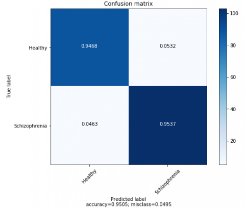
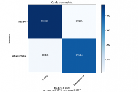
The confusion matrices given in Figure 12 clearly show that correct classification rate for diseased and non-diseased samples is high (>=0.94) while misclassification is very low with values close to 0 (<= 0.05) for both datasets.
Table 1. Performance results of the proposed method against Dataset A
|
Dataset A |
Precision |
Recall |
F1-score |
Support |
|
Healthy Control |
0.95 |
0.95 |
0.95 |
94 |
|
SZ Patient |
0.95 |
0.95 |
0.95 |
108 |
|
|
||||
|
Accuracy |
|
0.95 |
202 |
|
|
Macro avg |
0.95 |
0.95 |
0.95 |
202 |
|
Weighted avg |
0.95 |
0.95 |
0.95 |
202 |
Table 2. Performance results of the proposed method against Dataset A
|
Veri Seti B |
Precision |
Recall |
F1-score |
Support |
|
Healthy Control |
0.97 |
0.98 |
0.98 |
484 |
|
SZ Patient |
0.98 |
0.96 |
0.97 |
414 |
|
|
||||
|
Accuracy |
|
0.97 |
898 |
|
|
Macro avg |
0.97 |
0.97 |
0.97 |
898 |
|
Weighted avg |
0.97 |
0.97 |
0.97 |
898 |
An obtained high TPR and low FPR for a specific configuration does not mean a binary classifier is good at all threshold values and therefore may suffer from poor performance because of close values produced for “0” s and “1” s. However, this is not the case for the proposed method since AUC values are obtained as 0.95 and 0.974 for Dataset A and B, respectively (see Figure 13). That is, the produced values to represent “0” s and “1” s are very close to “0” and “1” and thus most of the threshold values suffice to discriminate between two. That makes the proposed method a robust classifier for most cases.
(a)
(b)
Figure 12. The confusion matrices of the proposed method for (a) Dataset A and (b) Dataset B
The Dataset A was previously evaluated by Phang et al. [17] which reported to reach a classification accuracy of 93.06%. Their method was a CNN model that used raw EEG signals as input. The method used an ensemble of 1D and 2D CNNs each of which classified the given signals by using different sets of features like brain connectivity features. The second dataset was also evaluated against a CNN model proposed by Oh et al. [6]. In their method, raw EEG signals are fed without a preprocessing to a CNN directly predicts the class value with an accuracy of 98.07%.
In comparison to these previous literature methods related to our work, our method outperforms most of them and performs comparably with one study [6]. As to our knowledge, due to reasons such as the lack of abundant SZ patient data available publicly, most methods measured the performance with a single set of data whereas our method is evaluated against two separate sets of data (children and adult). This clearly proves the robustness of the proposed method for different cases. Secondly, our improved performance with respect to methods that utilize raw EEG signals may be linked to the use of converting EEGs into spectrogram images which exhibit frequency information of the signal explicitly.
(a)
(b)
Figure 13. ROC for (a) Dataset A and (b) Dataset B
Furthermore, CNNs are designed to classify images that have spatial relations between pixels and mostly rely upon these spatial features while classifying an object. In a raw EEG signal, only temporal relationships are explicitly available.
A spectrogram being an image that keeps frequency and time information with spatial relationships is thus a more suitable input for a CNN model.
Furthermore, the proposed method in this study is capable of producing more human-interpretable outputs. In this context, when the spectrogram images for a healthy control and a SZ patient shown in Figure 7 and 8 are inspected, it can be seen that these spectrograms have differences such as different frequency values at different times.
However, it is hard for a human to generalize these differences for all samples in a dataset and formulize them quantitatively. In this regard, we attempt to reveal what these differences are by using a technique called Activation Maximization (AC) [32].
An AC image is an artificial image synthesized by iteratively finding the values that maximize the output of the network for a single class. Therefore, it can be thought of an ideal input that represents a class. Even though there are clear differences in AC images presented in Figure 14 for a healthy control and a SZ patient, these images only show that the network respond to spectrograms of different classes in a very diverse way.
It is because that the features seen in AC images are artificially generated to maximize the filter activation and therefore do not necessarily represent real spectrogram images.
Figure 14. Activization maximization images for (a) healthy control and (b) SZ patient
Figure 15. Grad-CAM images obtained from a set of individuals of (a) healthy controls and (b) SZ patients
Table 3. A summary of relevant literature methods that aims to automatically detect SZ patients
|
Year of study |
The study |
Methods |
Data |
Accuracy |
|
2015 |
Kim et al. [7] |
* Obtaining different frequency bands, *Calculation of spectral power, * Fast Fourier Transformation, *ROC analysis |
90 healthy control 90 SZ patient |
62.2% |
|
2015 |
Dvey-Aharon et al. [9] |
*Stockwell transformation, * “TFFO” (Time-Frequency transformation followed by Feature-Optimization) |
25 healthy control 50 SZ patient |
Between 92% and 93.9% |
|
2016 |
Johannesen et al. [11] |
*Statistical analysis over spectral power, *SVM classification |
12 healthy control 40 SZ patient |
87% |
|
2016 |
Santos-Mayo et al. [13] |
*EEGLAB feature extraction, *J5 feature extraction, *MLP and SVM classification |
31 healthy control 16 SZ patient |
MLP: 93.42% SVM: 92.23% |
|
2017 |
Thilakvathi B et al. [17] |
*Hannon entropy, *Spectral entropy, *Information entropy *higuchi’s fractal dimension, *Kolmogorov complexity and approximate entropy, *SVM classification |
23 healthy control 55 SZ patient |
88.5% |
|
2019 |
Aslan and Akın [15] |
*Wavelet, *Relative Wavelet Energy, * KNN classification |
39 healthy control 45 SZ patient
|
90% |
|
2019 |
Phang et al. [16] |
CNN |
39 healthy control 45 SZ patient
|
93.06% |
|
2019 |
Shu Lih Oh et al. [6] |
CNN |
14 healthy control 14 SZ patient |
98.07%
|
Therefore, as a second attempt, we utilized another technique called Gradient Weighted Activation Maps (Grad-CAM) [33] in order to understand what really differs for a healthy control and a SZ patient. In a Grad-CAM image, a color map is depicted on an input image where colors show the relevance of the region in the image with respect to the predicted class. Therefore, colors close to red on the image means that that region holds important spatial features for the predicted class. Figure 15 shows Grad-CAM images of different individuals grouped by class. The Grad-CAM images belong to the diseased group clearly reveal a pattern that is usually colors being centered in the middle of the image whereas in healthy control images high intensity colors either never appear or appear only at the top and bottom of the image.
Please note that the pattern shown in Figure 15 is common to other individuals not shown in the figure. Therefore, a few results can be inferred out of these images. First and foremost, frequency components matter in the discrimination of SZ patients and healthy controls. Moreover, the mid-level frequency components are the most important ones to discriminate SZ patients as almost all samples in this group has a similar pattern in the spectrogram region that represent mid-level frequency components.
Table 3 summarizes the relevant literature methods with respect the methodology and the accuracy reached. As a result of the table, it is clear that the method proposed in this paper outperforms all the methods mentioned in the table except one study conducted by Oh et al. [6] which has a comparable performance with the proposed method. Beyond the improved performance tested on two different datasets, the proposed method has several advantages over literature methods. Firstly, unlike the literature studies that utilize ML methods, it does not have a preprocessing stage to manually extract features. Furthermore, it does not need to preprocess spectrogram images. Secondly, its results are interpretable and reveals which frequency components matter for EEG recordings of SZ patients. Lastly, it has a simple pipeline, raw EEG signals are transformed into spectrograms which are then given to the CNN model.
In this study, a method is proposed to automatically diagnose SZ patients. The experiments conducted by use of two separate datasets prove that the method is capable of discriminating healthy controls and SZ patients in a robust and accurate way. The accuracy values reached by the method are 95% and 97% for Dataset A and B, respectively. With these results, the proposed method outperforms most of the methods in the relevant literature.
Furthermore, the proposed method reveals that analyzing frequency components in an EEG recording is a robust way of discriminating the SZ disease described as a brain disorder. Particularly, Grad-CAM images show that mid-level frequency components of an EEG record of a SZ patient show a specific pattern that makes the records separable. The method introduced in the paper can be used as a framework for CAD studies that attempt to detect certain diseases that are considered to have some trace in the EEG recordings.
The proposed method uses a state-of-art CNN architecture called VGG-16. As more CNN models are introduced frequently, it is obvious that new models may help improve the classification performance of the proposed method. Also, it should be noted that low complexity models with fewer layers/nodes/parameters with lower computational requirements will nonetheless be preferable even though they do not come with a performance advantage.
Data used in this study are taken from publicly available datasets each of which are used in previous studies. First data set is available at http://brain.bio.msu.ru/ eeg_schizophrenia.htm. The second one is accessible from https://repod.pon.edu.pl/dataset/eeg-in-schizophrenia.
[1] Buettner, R., Hirschmiller, M., Schlosser, K., Rössle, M., Fernandes, M., Timm, I.J. (2019). High-performance exclusion of schizophrenia using a novel machine learning method on EEG data. 2019 IEEE International Conference on E-health Networking, Application & Services (HealthCom), Bogota, Colombia, pp. 1-6. http://dx.doi.org/10.1109/HealthCom46333.2019.9009437
[2] Zhang, L. (2019). EEG signals classification using machine learning for the identification and diagnosis of schizophrenia. 2019 41st Annual International Conference of the IEEE Engineering in Medicine and Biology Society (EMBC), Berlin, Germany, pp. 4521-4524. http://dx.doi.org/10.1109/EMBC.2019.8857946
[3] Shim, M., Hwang, H.J., Kim, D.W., Lee, S.H., Im, C.H. (2016). Machine-learning-based diagnosis of schizophrenia using combined sensor-level and source-level EEG features. Schizophrenia Research, 176(2-3): 314-319. http://dx.doi.org/10.1016/j.schres.2016.05.007
[4] Cao, B., Cho, R.Y., Chen, D.C., Xiu, M.H., Wang, L., Soares, J.C., Zhang, X.Y. (2020). Treatment response prediction and individualized identification of first-episode drug-naïve schizophrenia using brain functional connectivity. Molecular Psychiatry, 25: 906-913. https://doi.org/10.1038/s41380-018-0106-5
[5] Jack Jr, C.R., Lowe, V.J., Weigand, S.D., Wiste, H.J., Senjem, M.L., Knopman, D.S., Shiung, M.M., Gunter, J.L., Boeve, B.F., Kemp, B.J., Weiner, M., Petersen, R.C., the Alzheimer's Disease Neuroimaging Initiative. (2009). Serial PIB and MRI in normal, mild cognitive impairment and Alzheimer’s disease: Implications for sequence of pathological events in Alzheimer’s disease. Brain, 132(5): 1355-1365. https://doi.org/10.1093/brain/awp062
[6] Oh, S.L., Vicnesh, J., Ciaccio, E.J., Yuvaraj, R., Acharya, U.R. (2019). Deep convolutional neural network model for automated diagnosis of schizophrenia using EEG signals. Applied Science, 9(14): 2870. https://doi.org/10.3390/app9142870
[7] Kim, J.W., Lee, Y.S., Han, D.H., Min, K.J., Lee, J., Lee, K. (2015). Diagnostic utility of quantitative EEG in un-medicated schizophrenia. Neuroscience Letters, 589: 126-131. https://doi.org/10.1016/j.neulet.2014.12.064
[8] Delorme, A., Makeig, S. (2004). EEGLAB: An open source toolbox for analysis of single-trial EEG dynamics including independent component analysis. Journal of Neuroscience Methods, 134(1): 9-21. https://doi.org/10.1016/j.jneumeth.2003.10.009
[9] Dvey-Aharon, Z., Fogelson, N., Peled, A., Intrator, N. (2015). Schizophrenia detection and classification by advanced analysis of EEG recordings using a single electrode approach. PLoS One, 10(4): e0123033. https://doi.org/10.1371/journal.pone.0123033
[10] Stockwell, R.G., Mansinha, L., Lowe, R.P. (1996). Localization of the complex spectrum: The S transform. IEEE Transactions on Signal Processing, 44(4): 998-1001. http://dx.doi.org/10.1109/78.492555
[11] Johannesen, J.K., Bi, J., Jiang, R., Kenney, J.G., Chen, C.M.A. (2016). Machine learning identification of EEG features predicting working memory performance in schizophrenia and healthy adults. Neuropsychiatric Electrophysiology, 2: 3. https://doi.org/10.1186/s40810-016-0017-0
[12] Guyon, I., Elisseeff, A. (2003). An introduction to variable and feature selection. The Journal of Machine Learning Research, 3: 1157-1182.
[13] Santos-Mayo, L., San-José-Revuelta, L.M., Arribas, J.I. (2016). A computer-aided diagnosis system with EEG based on the P3b wave during an auditory odd-ball task in schizophrenia. IEEE Transactions on Biomedical Engineering, 64(2): 395-407. https://doi.org/10.1109/TBME.2016.2558824
[14] Devijver, P.A., Kittler, J. (1982). Pattern Recognition: A Statistical Approach. Prentice Hall.
[15] Aslan, Z., Akın, M. (2019). Detection of schizophrenia on EEG signals by using relative wavelet energy as a Feature Extractor. UEMK 2019 4th International Energy & Engineering Congress, pp. 301-310.
[16] Thilakvathi, B., Shenbaga Devi, S., Bhanu, K., Malaippan, M. (2017). EEG signal complexity analysis for schizophrenia during rest and mental activity. Biomedical Research, 28(1).
[17] Phang, C.R., Ting, C.M., Noman, F., Ombao, H. (2019). Classification of EEG-based brain connectivity networks in schizophrenia using a multi-domain connectome convolutional neural network. arXiv Prepr. arXiv1903.08858.
[18] Aslan, Z. (2019). On the use of deep learning methods on medical images. The International Journal of Energy and Engineering Sciences, 3(2): 1-15.
[19] Hubel, D.H., Wiesel, T.N. (1968). Receptive fields and functional architecture of monkey striate cortex. The Journal of Physiology, 195(1): 215-243. http://dx.doi.org/10.1113/jphysiol.1968.sp008455
[20] Min, S., Lee, B., Yoon, S. (2017). Deep learning in bioinformatics. Briefings in Bioinformatics, 18(5): 851-869. http://dx.doi.org/10.1093/bib/bbw068
[21] Litjens, G., Kooi, T., Bejnordi, B.E., Setio, A.A.A., Ciompi, F., Ghafoorian, M., van der Laak, J.A.W.M., van Ginneken, B., Sánchez, C.I. (2017). A survey on deep learning in medical image analysis. Medical Image Analysis, 42: 60-88. http://dx.doi.org/10.1016/j.media.2017.07.005
[22] Goodfellow, I., Bengio, Y., Courville, A. (2016). Deep learning. MIT Press, 19: 305-307. http://dx.doi.org/10.1007/s10710-017-9314-z
[23] Prabhu, Understanding of Convolutional Neural Network (CNN) — Deep Learning.” [Online]. Available: https://medium.com/@RaghavPrabhu/understanding-of-convolutional-neural-network-cnn-deep-learning-99760835f148, accessed on 10-Jan-2020.
[24] Arsa, D.M.S., Susila, A.A.N.H., (2019). VGG16 in batik classification based on random forest. 2019 International Conference on Information Management and Technology (ICIMTech), 1: 295-299.
[25] Tindall, L., Luong, C., Saad, A. (2015). Plankton classification using vgg16 network.
[26] Yuan, L., Cao, J. (2017). Patients’ EEG data analysis via spectrogram image with a convolution neural network. International Conference on Intelligent Decision Technologies, pp. 13-21. http://dx.doi.org/10.1007/978-3-319-59421-7_2
[27] Borisov, S.V., Kaplan, A.Y., Gorbachevskaya, N.L., Kozlova, I.A. (2005). Analysis of EEG structural synchrony in adolescents with schizophrenic disorders. Human Physiology, 31: 255-261. https://doi.org/10.1007/s10747-005-0042-z
[28] Olejarczyk, E., Jernajczyk, W. (2017). Graph-based analysis of brain connectivity in schizophrenia. PLoS One, 12(11): e0188629. https://doi.org/10.1371/journal.pone.0188629
[29] Kingma, D.P., Ba, J. (2014). Adam: A method for stochastic optimization. arXiv Prepr. arXiv1412.6980.
[30] Raschka, S. (2014). An overview of general performance metrics of binary classifier systems. arXiv Prepr. arXiv1410.5330.
[31] Goutte, C., Gaussier, E. (2005). A probabilistic interpretation of precision, recall and F-score, with implication for evaluation. European Conference on Information Retrieval, pp. 345-359. http://dx.doi.org/10.1007/978-3-540-31865-1_25
[32] Kotikalapudi, R. (2007). keras-vis. GitHub, https://github.com/raghakot/keras-vis, accessed on 12 December 2019.
[33] Selvaraju, R.R., Cogswell, M., Das, A., Vedantam, R., Parikh, D., Batra, D. (2017). Grad-cam: Visual explanations from deep networks via gradient-based localization. Proceedings of the IEEE International Conference on Computer Vision, pp. 618-626. http://dx.doi.org/10.1007/s11263-019-01228-7