Hesam Akbari | Somayeh Saraf Esmaili*
© 2020 IIETA. This article is published by IIETA and is licensed under the CC BY 4.0 license (http://creativecommons.org/licenses/by/4.0/).
OPEN ACCESS
The electroencephalogram (EEG) signal is known as a nonlinear and complex signal. The EEG signal has very important information about brain activities and disorders which can detect by an accurate Computer-aided diagnosis system. The performance of the Computer-aided diagnosis system directly depends on using features in the classifiers. In this paper, we proposed nonlinear geometrical features for the classification of EEG signals. The normal, interictal and ictal EEG signals of the Bonn university EEG database are plotted in 2D space by a novel approach and considering their patterns, six features namely: area of the octagon (AOO), circle area (CA), the summation of vectors length (SVL), centroid to coordinate center (CTC), circular radius out of triangles (CRT) and triangle area (TA) are extracted on different aspects of distance in Cartesian space. Based on the Kruskal–Wallis statistical test, all of the features were found statistically significant in the discrimination of normal vs. ictal and interictal vs. ictal EEG signals (p-value≈0). Also, the edges of 2D projection EEG signals in the ictal group were sharper than normal and interictal groups. Besides, 2D projection of normal and interictal EEG signals has more regular geometrical shapes than the ictal group. Our proposed features were applied as input on support vector machine (SVM) and k-nearest neighbors (KNN) classifiers which resulted in more than 99% classification accuracy in a ten-fold cross-validation strategy.
ictal EEG signal, geometrical features, computer-aided diagnosis, SVM, KNN
Epilepsy is a common brain disorder due to abnormal activity of neurons. It normally affects more than 50 million of the population in the world who most of them are living in developing countries [1]. Doctors and neurologists can evaluate the brain nerve activity by analyzing the Electroencephalography (EEG) signal. In EEG records, epilepsy attacks have manifested themselves with spikes in the EEG signal which can be detected visually by the medical team [2]. Visual inspection of EEG records for the long-term to detect presence of epilepsy attacks by medical team are very boring, time consuming and prone to human error. Therefore, a Computer-aided diagnosis system for detection of epilepsy attacks in EEG signals is desirable [3]. For this purpose, for the past two decades, several machine learning methods based on the extraction of features from EEG signals have been developed in the literates. There is a direct relationship between the clinically significant feature extraction from EEG signals and the performance of machine learning which resulted to design an accurate Computer-aided diagnosis system. Traditionally, extracted features are categorized into three groups; including extracted features in time (T) domain, frequency (F) domain and time-frequency (T-F) domain. T domain features are extracted from EEG signal without any processing method on EEG signal. In other words, these features are evaluating EEG signal behaviors in T domain. T domain features like mean, median, mode, minimum, maximum, skewness, standard deviation, kurtosis, energy, correlation and histograms have been computed from EEG signal, previously [4-13]. The T domain cannot show many inherent behaviors of the EEG signal. For this reason, the EEG signal transforms from the T domain to the F domain. The spectrum shows the frequency components of EEG signals. Fast Fourier transforms (FFT) algorithm is the most used tool for representing frequency spectrum. Phase slope index, frequency moment signatures and mean frequency have been computed from EEG signals in the F domain [14, 15]. Although FFT is very useful for analyzing the spectrum, there is no relationship between the T domain and the F domain [16]. In other words, extracted features in the F domain are useful when the EEG signal is assumed stationary. But in essence, the EEG signal is complex and non-stationary and it can be assumed stationary only in the short-term. So, T-F approaches like wavelet transform and empirical mode decomposition was decomposed the EEG signals and several features including: entropy-based features (log energy, Shannon, threshold, norm), chaotic-based features (fractal dimension, Lyapunov exponent, centered correntropy, information potential) were extracted from EEG sub-bands as T-F domain features [17-22].
Expect of these traditional methods, researchers have suggested a few numbers of geometrical methods for the detection of epilepsy attaches by using second-order difference plot [23] and reconstructed phase space [24]. The EEG signals were decomposed to intrinsic mode functions (IMFs) by empirical mode decomposition, then the computation of the elliptical pattern of the second-order difference plot of IMFs was considered as a feature [23]. In similar research [24], the elliptical pattern of the reconstructed phase space of IMFs was considered as a feature. In other words, their works [23, 24] can be categorized in T-F methods, because EEG signals are decomposed by empirical mode decomposition.
Two methods of phase reconstructed phase space [23] and second-order difference plot [24] have been used in the past to represent the signal in two dimensions. The reconstructed phase space requires the estimation of two parameters, namely the time delay and the embedding dimension, which are calculated with mutual information (MI) and false nearest neighbor (FNN) [16, 25], respectively. The disadvantage of the phase space reconstruction method is that it is time-consuming because the MI and FNN calculations are extremely heavy [24].
The second-order difference plot method is suitable for showing signal variations because of drawing a two-dimensional signal difference [23]. But sometimes signal differentiation cannot give us good information about the behavior and dynamics of the signal itself.
For this reason, in this paper, we propose a novel method for plotting the signal in two dimensions, which, unlike phase space reconstruction, does not require any parameter, so it can quickly plot the signal in two dimensions. In addition, the proposed method shows the signal itself in two dimensions and the difference, unlike the second-order difference plot method. So, the behavior and dynamics of the signals can be better observed.
In this paper, the new features represent the complex behaviors of EEG signals in 2D space and their proposed patterns can discriminate the EEG signals in normal vs. ictal, and interictal vs. ictal groups better than traditional approaches, without any T-F methods [26].
The rest part of the paper is organized as follows: In section 2, geometrical method with used database, proposed 2D projection, area of the octagon (AOO), circle area (CA), the summation of vector length (SVL), centroid to centroid (CTC) and triangle area (TA) are covered. Results are provided in section 3. Finally, the discussion and conclusion of our paper are presented in section 4.
2.1 Used database
Our proposed method has been evaluated by known Bonn university EEG database which is freely downloadable from the http://epileptologie-bonn.de web site. There are five subsets of this database called A, B, C, D and E. Each sub-set has 100 EEG signals in a Text Document format (.txt). The duration of each EEG signal is 23.6 seconds, which was sampled at a rate of 173.61 Hz, so it has 4097 samples. The subset of A and B belong to five healthy subjects in eyes opened and closed conditions, respectively. The subset of C and D belong to five patients who had completed recovered from seizure control after surgery of epileptic locations. The subset E is composed of EEG signals with epileptic seizure activities that are observed in the epileptogenic zone. The signals in A and B sub-set are considered normal signals, C and D sub-sets are considered as interictal signals and signals in the E subset are considered as ictal signals. More details about the Bonn university EEG database can be found by Andrzejak et al. [27].
2.2 Proposed 2D projection
In this work, 4096 sample points of EEG signals were selected for evaluating our proposed method. All the calculations of our proposed method are carried out using the MATLAB software, also any tool box not used. In this paper, a geometrical non-linear method is developed which is directly depended to the number of EEG samples. By assuming that EEG signal be x(n)=[x1;x2;x3;…;xn], the EEG signals should be evolved into 2D projection with the following formula:
$X(m)=\left[x_{1} ; x_{3} ; x_{5} ; \ldots ; x_{4095}\right]$ (1)
$Y(m)=\left[x_{2} ; x_{4} ; x_{6} ; \ldots ; x_{4096}\right]$ (2)
2D Projection $(m)=[X(m), Y(m)]=\left[\left(x_{1}, x_{2}\right)_{1} ;\left(x_{3}, x_{4}\right)_{2} ; \ldots ;\left(x_{n-1}, x_{n}\right)_{m}\right]$ (3)
where, n is the lengths of the input signal x(n) and m is the 2D projection points and equal to n/2 (i.e. 2048 points which are mapped on Cartesian space).
Figure 1 shows a sample of 2D projection of normal, interictal and ictal EEG signals. Due to 2D projection of EEG signal pattern, we can compute the significant geometrical features to discrimination of ictal EEG signals from normal and interictal EEG signals.
Figure 1. 2D projection of the normal, interictal and ictal EEG signals
2.3 Area of octagon (AOO)
It is clear from Figure 1 that the 2D projection of EEG signals has geometrical patterns. It motivates us to compute the area of geometrical patterns as discrimination features. So, seems that the area of the octagon (AOO) of the 2D projection of EEG signals can give useful diagnostic feature. The AOO of 2D projection can be computed as follows [28]:
$M_{y^{2}}=(1 / M) \sum_{m=0}^{M-1}[Y(m)]^{2}$ (4)
$M_{x y}=(1 / M) \sum X(m) Y(m)$ (5)
$M_{s u m^{2}}=M_{X^{2}}+M_{Y^{2}}$ (6)
$M_{p r d^{2}}=M_{X^{2}} \times M_{Y^{2}}$ (7)
$D=\left[M_{s u m^{2}}-4\left(M_{p r d^{2}}-M_{X Y^{2}}\right)\right]^{1 / 2}$ (8)
$D i a=\left[3\left(M_{s u m^{2}}+D\right)\right]^{1 / 2}$ (9)
The AOO is obtained from Figure 2 as given below.
Figure 2. The octagon for AOO calculation
In the above Figure 2 From ΔABC, as all sides are equal in an octagon,
$S^{2}=|A C|^{2}+|B C|^{2}$ (10)
Therefore
$|A C|=S / \sqrt{2}$ (11)
where, ‘S’ is the sides of the octagon. In general, Diameter of the octagon is given by
Diameter $=S+2(S \sqrt{2})$ (12)
since $S=$Diameter $/(1+\sqrt{2})$ (13)
Area of octagon $=2(1+\sqrt{2}) \times S^{2}$ (14)
On substituting ‘S’ value in AOO
$A O O=\frac{2}{1+\sqrt{2}} \times D i a^{2}$ (15)
2.4 Circle Area (CA)
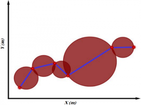
It can observe from Figure 1 that 2D projection of ictal EEG signal occupies more area than normal and intellectual groups. It mentioned to us that area computation can give useful diagnostic feature. Every two successive points on 2D projection, make a vector and each vector can make a circle with diameter D which equal to the vector length. In this work, the summation of circle areas using consecutive vectors is computed as a feature. The summation of circle areas using consecutive vectors is defined as:
$C A=\sum_{i=1}^{n-3} \frac{\pi}{2}\left(\left(x_{i+2}-x_{i}\right)^{2}+\left(x_{i+3}-x_{i+1}\right)^{2}\right)$ (16)
where, n denote to the samples of input EEG signal x(n); also, (xi, xi+1), (xi+2, xi+3), indicated to coordinate the two successive points on the 2D projection of EEG signals. Besides, CA is a summation of the circle area using consecutive vectors. The summation area of brown circles in Figure 3 is considered as a feature.
Figure 3. Illustration of CA as s feature
2.5 Summation of vectors length (SVL)
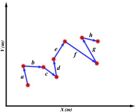
For quantification EEG signal amplitude changes in the time domain, we can compute the summation of successive vector lengths which make by the consecutive points on the 2D projection of EEG signals. In other words, we calculate the summation of consecutive vector length as a feature. It's defined as follows:
$S V L=\sum_{i=1}^{n-3} \sqrt{\left(x_{i+2}-x_{i}\right)^{2}+\left(x_{i+3}-x_{i+1}\right)^{2}}$ (17)
where, n denote to the samples of input EEG signal x(n); also, (xi, xi+1), and (xi+2, xi+3) indicated to coordinate the two successive points on 2D projection of EEG signals which make a vector. Besides, SVL is the summation of successive vector lengths. The summation distance of a, b, c, d, e, f, g and h vector length in Figure 4 are considered as a feature.
Figure 4. Illustration of SVL as s feature
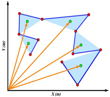
2.6 Centroid to Coordinate Center (CTC)
Every three successive points in the 2D plan make a triangle. So, points on the 2D projection of EEG signals can evolve into successive triangles. The distance between the center of the triangle and coordinate center can give useful diagnostic considering to the pattern of EEG signals in 2D space, because of ictal EEG signals that have occupied more area than normal and interictal EEG signals. The coordinates of the center of a triangle with (xi, xi+1), (xi+2, xi+3) and (xi+4, xi+5) edges can be computed as follow [34]:
$X_{c}=\frac{x_{i}+x_{i+2}+x_{i+4}}{3}$ (18)
$Y_{C}=\frac{x_{i+1}+x_{i+3}+x_{i+5}}{3}$ (19)
where, (XC, YC) denote to the triangle center coordinate. So the summation of centroid to coordinate center (CTC) distance of successive triangles can be defined as follows:
$C T C=\sum_{i=1}^{n} \sqrt{\left[X_{C}\right]^{2}+\left[Y_{C}\right]^{2}}$ (20)
where, u denote the number of successive triangles on 2D projection of EEG signals that is equal to 1023 which make with 2047 points.
The summation length of orange vectors in Figure 5 is considered as a feature.
Figure 5. Illustration of CTC as s feature
2.7 Circular radius out of triangles (CRT)
We said that each three successive points on coordinate plane make a triangle. We can draw a circle with radius r out of the each of triangle. In this paper, we are computed the summation of radius of the circles out of successive triangles as a feature.
Assuming that (xi, xi+1), (xi+2, xi+3) and (xi+4, xi+5) be three edges of a triangle on 2D space, then three sides of triangle are calculated as follow:
$a=\sqrt{\left(x_{i+2}-x_{i}\right)^{2}+\left(x_{i+3}-x_{i+1}\right)^{2}}$ (21)
$b=\sqrt{\left(x_{i+4}-x_{i+2}\right)^{2}+\left(x_{i+5}-x_{i+3}\right)^{2}}$ (22)
$c=\sqrt{\left(x_{i}-x_{i+4}\right)^{2}+\left(x_{i+1}-x_{i+5}\right)^{2}}$ (23)
where, a, b and c denote to three sides of first triangle. So, the triangle area can be calculated by the Heron principle as follow:
$\operatorname{area}=\sqrt{\frac{(a+b+c)}{2}+\frac{(-a+b+c)}{2}+\frac{(a-b+c)}{2}+\frac{(a+b-c)}{2}}$ (24)
Finally, the radius of circle out of first triangle is calculated as:
$r=\frac{a \times b \times c}{4 \times a r e a}$ (25)
In this work, the summation of the circular radius out of the successive triangles is computed as a feature as follow:
$C R T=\sum_{i=1}^{u} r_{i}$ (26)
where, u denote the number of successive triangles on the 2D projection of EEG signals and it is equal to 1023 which makes with 2047 points. The CTC and SVL are similar to CRT with this difference, that SVL and CTC quantify the variability of amplitude in the time domain, but CRT quantifies the self-similarity of the EEG signals on 2D projection plan with more flexibility than cross-correlation [8]. Although the SVL and CTC evaluate the variability of amplitude, SVL is sensitive to CTC. On the other hand, CTC can be more useful than SVL in ictal detection when EEG signal has baseline noise.
Figure 6. Illustration of CRT as s feature
The summation raduis of brown circles intriangles in Figure 6 is considered as a feature.
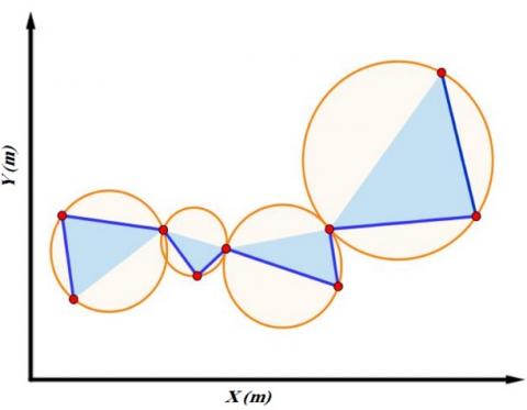
2.8 Triangle area (TA)
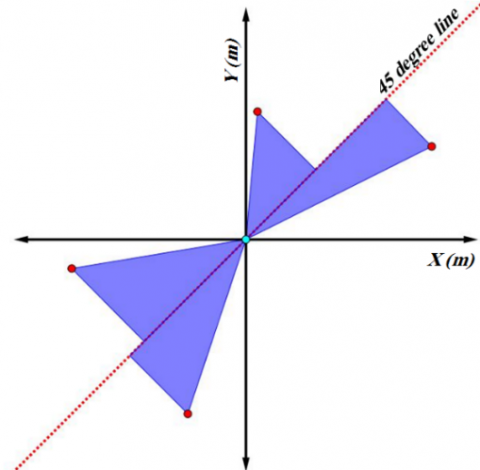
It is clear from Figure 1 that the scatter of points of EEG signals on the 2D projection plane is more on y=x and y=-x lines. For quantifying the scatter of points on y=x line, we computed the shortest distance of each point from 45degree line (shD) and for quantifying the scatter of points on y=-x line, distance of each point from coordinate center (crD) is computed. To combination of the shD and crD, we computed the area of a triangle which the shD and crD are two sides of it. With having the two sides of a right-angled triangle, we can compute the third side by the Pythagorean Theorem. The shD and crD of (xi, xi+1) point on EEG signals on 2D space can be defined as:
$s h D=\frac{\left|x_{i}-x_{i+1}\right|}{\sqrt{2}}$ (27)
$c r D=\sqrt{x_{i}^{2}+x_{i+1}^{2}}$ (28)
where, n denote to the samples of input EEG signal x(n). So, with having the two sides of triangle, the third side is calculated as follow:
$c r D^{2}=s h D^{2}+L^{2}$ (29)
Finally the triangle area can be calculated as follow:
$S=\frac{\operatorname{sh} D \times L}{2}$ (30)
In this work the summation area of triangles is used as a feature. It defined for 2D projection of EEG signals as follow:
$T A=\sum_{i=1}^{n} S_{i}$ (31)
where, n denote to the samples of input EEG signal x(n); also, TA is the summation of triangle areas. The summation area of blue triangles in Figure 7 is considered as a feature.
Figure 7. Illustration of TA as s feature
2.9 Classifiers
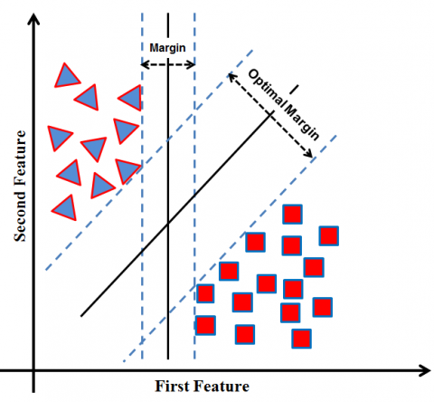
For classification of geometrical features, we employed two well-known classifiers, namely: support vector machine (SVM) and k-nearest neighbors (KNN) [3, 29, 30]. In the binary SVM classifier, input features are mapped to hyper dimensional space using kernel function; then a hyperplane with a maximum margin (optimal margin) is separated the features in two classes [29, 30]. KNN is a simple classifier with fast implementation [3]. In binary KNN classifier, first the training data of both classes are sorted. Then, the test data can be classified in the first or second group with considering to its K closed training data [3, 17]. That way, the test data belongs to classes that have more members among K closed neighbors (i.e. K closed test data). The kernel function and distance metric have a direct relationship in the correct classification of test data in SVM and KNN classifiers, respectively. In this work, radial basis function (RBF) and city-block are applied as kernel function and distance metric in SVM and KNN classifiers, respectively. Figure 8 and Figure 9 are explained the SVM and KNN algorithms in the binary classification by assuming that two features from each group are extracted. It can be understood form Figure 8 that the optimal margin (best hyperplane) can separate two classes better than the other margin. In Figure 9, the first, second, third and fourth circles around test data determine the one, seven, fourteen and twenty-one closed training data. The test data belongs to classes A, B, A and B with assuming that K is 1, 7, 14 and 21, respectively.
Figure 8. Illustration of the SVM algorithm as a used classifier
Figure 9. Illustration of the KNN algorithm as a used classifier
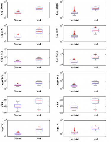
In this paper, we proposed novel non-linear geometrical features in order to discrimination of EEG signals in two classification tasks, including: normal vs. ictal (i.e. AB vs. E) and interictal vs. ictal (i.e. CD vs. E). P-value evaluates the ability of features in order to discriminate between the two classes [3]. In the present study, Kruskal–Wallis statistical test is applied to p-value computation [3, 15-19, 22, 24, 28, 30]. The kruskalwallis function in MATLAB is used for p-value computation. Features with less than 0.001 the p-value can be considered as clinically significant features in designing a Computer-aided diagnosis system [31-33]. In other word, lesser p-value indicates to better ability of features in the discrimination of groups [3, 16, 30]. In this work, we computed the p-values for normal vs. ictal and interictal vs. ictal groups. Also, the box plot is employed in showing the minimum, first quartile, median, third quartile, and maximum values of the extracted features. The mean and standard deviation of features are written in the Table 1 and resulted p-values are written in the Table 2. Also, box plots of features are shown in Figure 10.
Figure 10. Box plot of features
Clearly can be understood from Table 1, the mean values of the extracted features in normal, interictal and ictal EEG signals are significantly different with together. Also, it can be observed from Table 2 that the most of the p-values are very near to zero. Since the p-values for all properties are very close to zero, this means that the extracted property has a high ability to separate the two groups. In addition, in Table 2 the mean value of the features in the ictal signal is significantly larger than the mean value of the features in the normal and intractal signal. Given the low p-value values in Table 1, it can be said that all the features can be well defined in the classification task defined as normal vs. ictal, and interictal vs. ictal. This can also be obtained by analyzing Table 1, since the mean value in all features extracted from ictal signals is significantly larger than normal and Interictal signals. This can also be seen by examining the feature plots in Figure 10, since the box plot of all features for ictal signals is significantly larger than the box features for normal and interictal signals.
Table 1. Mean and standard deviation of features
|
Feature |
Normal |
Interictal |
Ictal |
|
AOO |
4.94E+06 ±3.41E+06 |
7.74E+06 ±2.09E+07 |
1.53E+08 ±1.32E+08 |
|
CA |
2.07E+07 ±1.77E+07 |
9.28E+06 ±1.98E+07 |
7.25E+08 ±8.88E+08 |
|
SVL |
9.05E+04 ±3.61E+04 |
4.91E+04 ±2.71E+04 |
4.26E+05 ±2.66E+05 |
|
CTC |
1.22E+05 ±4.58E+04 |
1.39E+05 ±8.64E+04 |
6.38E+05 ±2.94E+05 |
|
CRT |
4.79E+09 ±8.23E+09 |
1.06E+10 ±8.68E+10 |
4.93E+12 ±7.60E+12 |
|
TA |
8.41E+05 ±6.08E+05 |
6.85E+05 ±1.55E+06 |
2.62E+07 ±2.65E+07 |
Table 2. Resulted p-values
|
Feature |
Normal vs. Ictal |
Interictal vs. Ictal |
|
AOO |
3.78E-45 |
7.81E-43 |
|
CA |
1.29E-42 |
3.00E-44 |
|
SVL |
1.24E-39 |
2.56E-44 |
|
CTC |
4.0E-45 |
8.43E-43 |
|
CRT |
1.34E-43 |
1.16E-43 |
|
TA |
4.11E-44 |
5.82E-41 |
The box plot of the features is illustrated in Figure 10, in which the ictal EEG signals revealed higher AOO, CA, SVL, CTC, CRT and TA values than normal and interictal EEG signals (notice that expect of CRT box plot, the other box plots are illustrated the logarithmic values of the features). These reasons tell us that these nonlinear geometrical features can leaded us in designing an accurate Computer-aided diagnosis system. Hence, SVM and KNN classifiers are employed for designing a Computer-aided diagnosis system.
These reasons tell us that these three nonlinear geometrical features can leaded us in designing an accurate Computer-aided diagnosis system. Hence, SVM and KNN classifiers are employed for classification and designing a Computer-aided diagnosis system.
By assuming the EEG signals in ictal and non-ictal groups (i.e. normal and interictal be non-ictal in normal vs. ictal and interictal vs. ictal classification task, respectively), then the out-put of classifier is in one of the following conditions [3, 17, 24]:
TP (true positive): when ictal EEG signal is identified as ictal EEG signal.
TN (true negative): when non-ictal EEG signal is identified as non-ictal EEG signal.
FP (false positive): when non-ictal EEG signal is identified as ictal EEG signal.
FN (false positive): when ictal EEG signals is identified as non- ictal EEG signal.
With these parameters, accuracy (ACC), sensitivity (SEN) and specificity (SPE) can be defined as follow [3, 17, 24]:
$A C C=\frac{T P+T N}{T P+T N+F P+F N} \times 100$ (33)
$S E N=\frac{T P}{T P+F N} \times 100$ (34)
$S E N=\frac{T N}{T N+F P} \times 100$ (35)
In general, k-fold cross-validation [17, 24] is used to break the data into train and test to be used by the classifier. Actually, for the k-fold cross-validation, k time, k- 1 subset is used to train, and one resume subset is used to test the classifier. Finally, the mean value of ACC, SEN and SPE parameters are reported. Most of the articles that we wanted to compare our method with them used cross-validation technique [10, 11, 13, 22-24]. For this reason, we also used 10-fold cross-validation to analyze the results under almost equal conditions. The objective parameters for SVM and KNN classifiers with geometrical features are written in the Table 3 and Table 4, respectively.
The sigma value of RBF is varied from 0.1 to 1 by 0.1 step and number of k is varied from 1 to 9 by 2 step which the optimal ACC value for SVM and KNN classifier is obtained then sigma is chosen to 0.1 and number of k is chosen to 5, respectively. Besides, the ACC in Table 2 and 3 are resulted by one feature (i.e. feature vector has one array). With according to the resulted ACC, it can be observed that SVM and KNN classifier is better in order to normal vs. ictal and interictal vs. ictal classification, respectively.
Hence, the feature vector length in normal vs. ictal classification task is increased to two by combination of CTC and the other features in SVM classifier. The resulted parameters are written in Table 5, in which the combination of CTC with other features are resulted to perfect average classification ACC of 99.13%.
Table 3. Performance of geometrical features with SVM classifier
|
Feature vector |
Normal vs. Ictal |
||
|
ACC (%) |
SEN (%) |
SPE (%) |
|
|
CTC |
99.33 |
99 |
99.50 |
|
AOO |
98.33 |
98 |
98.5 |
|
CA |
98 |
97 |
93.5 |
|
TA |
95.66 |
95 |
96 |
|
SVL |
94.33 |
93 |
95 |
|
CRT |
93.66 |
81 |
100 |
|
Average. value |
96.55 |
93.83 |
97.08 |
|
Feature vector |
Interictal vs. Ictal |
||
|
ACC (%) |
SEN (%) |
SPE (%) |
|
|
AOO |
95.66 |
100 |
94 |
|
CA |
97.66 |
99 |
97 |
|
TA |
96.33 |
99 |
95 |
|
SVL |
97.33 |
97 |
97.5 |
|
CTC |
95.33 |
93 |
93.50 |
|
CRT |
92.66 |
81 |
98.50 |
|
Average. value |
95.82 |
94.83 |
95.91 |
Table 4. Performance of geometrical features with KNN classifier
|
Feature vector |
Normal vs. Ictal |
||
|
ACC (%) |
SEN (%) |
SPE (%) |
|
|
SVL |
93 |
89 |
95.50 |
|
CA |
93.66 |
90 |
96.5 |
|
CTC |
99 |
98 |
99.50 |
|
TA |
96 |
91 |
98.50 |
|
AOO |
98.67 |
98.00 |
99.00 |
|
CRT |
94.33 |
90 |
97.50 |
|
Average. value |
95.77 |
92.66 |
97.75 |
|
Feature vector |
Interictal vs. Ictal |
||
|
ACC (%) |
SEN (%) |
SPE (%) |
|
|
SVL |
97.66 |
97 |
98 |
|
CA |
97.33 |
98 |
97.5 |
|
TA |
96.33 |
96 |
96.50 |
|
CTC |
95.66 |
98 |
94.50 |
|
AOO |
95.67 |
96.00 |
95.50 |
|
CRT |
96 |
96 |
96.50 |
|
Average. value |
96.44 |
96.83 |
96.41 |
Table 5. Performance of SVM classifier in Normal vs. Ictal classification task with two features
|
Feature vector |
Normal vs. Ictal |
||
|
ACC (%) |
SEN (%) |
SPE (%) |
|
|
CTC, AOO |
99 |
99 |
99.50 |
|
CTC,CA |
99 |
98 |
99.50 |
|
CTC, CRT |
99.33 |
99 |
99.50 |
|
CTC,SVL |
99.33 |
98 |
100 |
|
CTC,TA |
99 |
98 |
99.50 |
|
Average. value |
99.13 |
98.40 |
99.60 |
In the same way, ACC of KNN classifier in interictal vs. ictal classification task can be improved. For this propose, arrays of feature vector in KNN classifier are increased to two by a combination of SVL with the other features. Performance of KNN classifier with this feature vector are written in Table 6.
Table 6. Performance of KNN classifier in Interictal vs. Ictal classification task with two features
|
Feature vector |
Normal vs. Ictal |
||
|
ACC (%) |
SEN (%) |
SPE (%) |
|
|
SVL,CTC |
97.33 |
99 |
96.50 |
|
SVL,CA |
97.33 |
98 |
97.5 |
|
SVL,TA |
96.67 |
97 |
97 |
|
SVL,CRT |
96.33 |
96 |
97 |
|
SVL,AOO |
96 |
96 |
96 |
|
Average. value |
96.73 |
97.20 |
96.80 |
The KNN classifier resulted in average 97.06% of ACC with two features. Also, to improve the ACC of the classifier, we investigated the combination of several geometrical features under 10-fold cross-validation conditions, which with three AOO, CA, SVL and CTC features vector, and reached a high of 99% ACC.
Epilepsy is a common brain disorder due to abnormal activity of neurons. It normally affects more than 50 million of the population in the world who most of them are living in developing countries [1]. Although doctors and neurologists can detect the of epilepsy attaches by visual analyzing of Electroencephalography (EEG), but visual inspection of EEG records for the long-term are very boring, time consuming and prone to human error. Hence, an accurate Computer-aided diagnosis system for detecting the presence of epilepsy attaches in EEG signals is desirable. In this paper, six novel nonlinear geometrical features namely: area of octagon (AOO), circle area (CA), summation of vectors length (SVL), centroid to coordinate center (CTC), circular radius out of triangles (CRT) and triangle area (TA) were proposed to detection of epilepsy attach in EEG signal.
For this propose, these features were employed to discrimination of ictal EEG signals from normal and interictal EEG signals in two classification tasks including: normal vs. ictal, and interictal vs. ictal.
Ictal, interictal and normal EEG signals were selected from well-known Bonn university database which has 200 normal (A and B sub-sets), 200 interictal (C and D sub-sets) and 100 ictal (E sub-set) EEG signals [27]. We showed that our 2D projection method can be used as a useful approach to illustration of complexity of EEG signals. Considering to Figure 1 the 2D projection of ictal EEG signals was occupied more space than normal and interictal EEG signals; this result has been reported in previous studies by drawing the EEG signals on 2D plane using second order difference plot [23] and phase space reconstructed [24]. Also, the edges of 2D projection EEG signals in ictal group were sharper than normal and interictal groups. Ray [2] said that ictal is manifesting itself with spikes in the EEG signal. For this reason, corresponding to Figure 1, the ictal EEG signals on the 2D projection were revealed by sharp edges. It can be observed from Figure 1, that 2D projection of normal and interictal EEG signals have more regular geometrical shapes. It may be due to synchronous response of brain neurons, which gives rise ictal parts in EEG signals. Support vector machine (SVM) and k-nearest neighbors (KNN) classifiers were employed for evaluation of accuracy (ACC), sensitivity (SEN) and specificity (SPE) of the proposed geometrical features. Corresponding to the Table 1 and 2, features were extremely severely statistically significant. Our proposed method resulted to more than 99% classification ACC in both classification task. We have compared our proposed method with existing studies on the same database in Table 7.
Table 7. Comparison of proposed method with the exiting work
|
Reference Year |
Used cross validation |
Used Sub-sets |
ACC (%) |
|
[9] (2012) |
No |
A vs. E B vs. E C vs. E D vs. E |
93.55 82.88 88.00 79.94 |
|
[10] (2014) |
10-fold |
A vs. E B vs. E C vs. E D vs. E |
99 97 98 93 |
|
[11] (2011) |
10-fold |
A vs. E B vs. E C vs. E D vs. E |
99.69 96.78 97.69 93.91 |
|
[12] (2010) |
No |
A, B vs. E C, D vs. E |
96 94 |
|
[20] (2014) |
No |
C, D vs. E |
95.33 |
|
[23] (2014) |
10-fold |
C, D vs. E |
97.75 |
|
[24] 2015 |
10-fold |
C, D vs. E |
98.67 |
|
[13] (2016) |
10-fold |
A, B vs. E C, D vs. E |
99.18 95.15 |
|
[19] 2019) |
No |
A vs.E C vs. E D vs. E C, D vs. E |
98.10 95.50 93.80 95.10 |
|
[22] (2017) |
10-fold |
C, D vs. E |
97.5 |
|
Proposed method |
10-fold |
A, B vs. E C, D vs. E |
99.26 99 |
[1] Acharya, U.R., Sree, S.V., Suri, J.S. (2011). Automatic detection of epileptic EEG signals using higher order cumulant features. International Journal of Neural Systems, 21(5): 403-414. https://doi.org/10.1142/S0129065711002912
[2] Ray, G.C. (1994). An algorithm to separate nonstationary part of a signal using mid-prediction filter. IEEE Trans. Signal Processing, 42(9): 2276-2279. https://doi.org/10.1109/78.317850
[3] Sharma, M., Achuth, P.V., Puthankattil, S.D., Deb, D., Acharya, U.R. (2018). An automated diagnosis of depression using three-channel bandwidth-duration localized wavelet filter bank with EEG signals. Cognitive Systems Research, 52: 508-520. https://doi.org/10.1016/j.cogsys.2018.07.010
[4] Runarsson, T.P., Sigurdsson, S. (2005). On-line detection of patient specific neonatal seizures using support vector machines and half-wave attribute histograms. In: CIMCA-IAWTIC, 2: 673-677. https://doi.org/10.1109/CIMCA.2005.1631546
[5] Baldominos, A., Ramón-Lozano, C. (2017). Optimizing EEG energy-based seizure detection using genetic algorithms. In 2017 IEEE Congress on Evolutionary Computation (CEC), pp. 2338-2345. https://doi.org/10.1109/CEC.2017.7969588
[6] Shanir, P.P, Khan, Y.U., Farooq, O. (2015). Time domain analysis of EEG for automatic seizure detection. Emerging Trends in Electrical and Electronics Engineering.
[7] Alotaiby, T.N., Alshebeili, S.A., El-Samie, F.E.A., Alabdulrazak, A., Alkhnaian, E. (2017). Channel selection and seizure detection using a statistical approach. International Conference on Electronic Devices, Systems and Applications, pp. 2-5. https://doi.org/10.1109/ICEDSA.2016.7818505
[8 Mursalin, M., Zhang, Y., Chen, Y., Chawla, N.V. (2017). Automated epileptic seizure detection using improved correlation-based feature selection with random forest classifier. Neurocomputing, 241: 204-214. https://doi.org/10.1016/j.neucom.2017.02.053
[9] Nicolaou, N., Georgiou, J. (2012). Detection of epileptic electroencephalogram based on permutation entropy and support vector machines. Expert Systems With Applications, 39(1): 202-209. https://doi.org/10.1016/j.eswa.2011.07.008
[10] Zhu, G., Li, Y., Wen, P. (2014). Epileptic seizure detection in EEGs signals using a fast weighted horizontal visibility algorithm. Computer Methods and Programs in Biomedicine, 115(2): 64-75. https://doi.org/10.1016/j.cmpb.2014.04.001
[11] Siuly, S., Li, P., Wen, Y. (2011). Clustering technique-based least square support vector machine for EEG signal classification. Computer Methods and Programs in Biomedicine, 104(3): 358-372. https://doi.org/10.1016/j.cmpb.2010.11.014
[12] Altunay, S., Telatar, Z., Erogul, O. (2010). Epileptic EEG detection using the linear prediction error energy. Expert Systems with Applications, 37(8): 5661-5665. https://doi.org/10.1016/j.eswa.2010.02.045
[13] Swami, P., Gandhi, T.K., Panigrahi, B.K., Tripathi, M., Anand, S. (2016). A novel robust diagnostic model to detect seizures in electroencephalography. Expert Systems with Applications, 56: 116-130. https://doi.org/10.1016/j.eswa.2016.02.040
[14] Khamis, H., Mohamed, A., Simpson, S. (2013). Frequency–moment signal tures: A method for automated seizure detection from scalp EEG. Clinical Neurophysiology, 124(12): 2317-2327. https://doi.org/10.1016/j.clinph.2013.05.015
[15] Singh, P., Pachori, R.B. (2017). Classification of focal and non focal EEG signals using features derived from fourier-based rhythms. Journal of Mechanics in Medicine and Biology, 17(7): 1740002. https://doi.org/10.1142/S0219519417400024
[16] Gupta, V., Bhattacharyya, A., Pachori, R.B. (2019). Automated identification of epileptic seizures from EEG signals using FBSE-EWT method. Biomedical Signal Processing-Advances in Theory, Biomedical Signal Processing, 157-179. https://doi.org/10.1007/978-981-13-9097-5_8
[17] Sharma, M., Pachori, R.B. (2017). A novel approach to detect epileptic seizures using a combination of tunable-Q wavelet transform and fractal dimesnion. Journal of Mechanics in Medicine and Biology, 17(7): 1-21. https://doi.org/10.1142/S0219519417400036
[18] Sharma, M., Pachori, R.B., Acharya, U.R. (2017). A new approach to characterize epileptic seizures using analytic time-frequency flexible wavelet transform and fractal dimension. Pattern Recognition Letters, 94: 172-179. https://doi.org/10.1016/j.patrec.2017.03.023
[19] Rafik1, D., Larbi, B. (2019). Autoregressive modeling based empirical mode decomposition (EMD) for epileptic seizures detection using EEG signals. Traitement du Signal, 36(3): 273-279. https://doi.org/10.18280/ts.360311
[20] Joshi, V., Pachori, R.B., Vijesh, A. (2014). Classification of ictal and seizure free EEG signals using fractional linear prediction. Biomedical Signal Processing and Control, 9: 1-5. https://doi.org/10.1016/j.bspc.2013.08.006
[21] Rizi, F.Y. (2019). A review of notable studies on using Empirical Mode Decomposition for biomedical signal and image processing. Signal Processing and Renewable Energy, 3(4): 89-113.
[22] Patidar, S., Panigrahi, T. (2017). Detection of epileptic seizure using Kraskov entropy applied on tunable-Q wavelet transform of EEG signals. Biomedical Signal Processing and Control, 34: 74–80. https://doi.org/10.1016/j.bspc.2017.01.001
[23] Pachori, R.B., Patidar, S. (2014). Epileptic seizure classification in EEG signals using second-order difference plot of intrinsic mode functions. Comput. Methods Programs Biomed, 113(2): 494-502. https://doi.org/10.1016/j.cmpb.2013.11.014
[24] Sharma, R., Pachori, R.B. (2015). Classification of epileptic seizures in EEG signals based on phase space representation of intrinsic mode functions. Expert Systems with Applications, 42(3): 1106-1117. https://doi.org/10.1016/j.eswa.2014.08.030
[25] Kantz, H., Schreiber, T. (2004). Nonlinear Time Series Analysis. U.K., Cambridge University Press, 7: https://doi.org/10.1017/CBO9780511755798
[26] Roulston, M.S. (1999). Estimating the errors on measured entropy and mutual information. Physica D: Nonlinear Phenomena, 125(3-4): 285-294. https://doi.org/10.1016/S0167-2789(98)00269-3
[27] Andrzejak, R.G., Lehnertz, K., Mormann, F., Rieke, C., David, P., Elger, C.E. (2001). Indications of nonlinear deterministics and finite-dimensional structures in time series of brain electrical activity: Dependence on recording region and brain state. Physical Review E, 64(6): 061907. https://doi.org/10.1103/PhysRevE.64.061907
[28] Krishnaprasanna, R., Vijayabaskar, V. (2019). Classification of focal and non-focal EEG signal using an area of octagon method. International Journal of Engineering and Advanced Technology (IJEAT), 9(1): 1832-1838. https://doi.org/10.35940/ijeat.A1450.109119
[29] Sadiq, M.T., Yu, X., Yuan, Z., Fan, Z., Rehman, A.U., Li, G., Xiao, G. (2019). Motor imagery EEG signals classification based on mode amplitude and frequency components using empirical wavelet transform. IEEE Access, 7: 127678-127692. https://doi.org/10.1109/ACCESS.2019.2939623
[30] Tripathy, R.K., Bhattacharyya, A., Pachori, R.B. (2019) A novel approach for detection of myocardial infarction from ECG signals of multiple electrodes. IEEE Sensors Journal, 19(12): 4509-4517. https://doi.org/10.1109/JSEN.2019.2896308
[31] Bhattacharyya, A., Sharma, M., Pachori, R.B., Sircar, P., Acharya, U.R. (2018). A novel approach for automated detection of focal EEG signals using empirical wavelet transform. Neural Computing and Applications, 29(8): 47-57. https://doi.org/10.1007/s00521-016-2646-4
[32] Behbahani, S., Moridani, M.K. (2015). Non-linear Poincaré analysis of respiratory efforts in sleep apnea. Bratisl Lek Listy, 116(7): 426-432. https://doi.org/10.4149/bll_2015_081
[33] Behbahani, S., Dabanloo, N.J., Nasrabadi, A.M., Dourado, A. (2016). Classification of ictal and seizure-free HRV signals with focus on lateralization of epilepsy. Technol Health Care, 24(1): 43-56. https://doi.org/10.3233/THC-151072
[34] Azizi, A. Moridani, M.K., Saeedi. A. (2019). A novel geometrical method for depression diagnosis based on EEG signals. 2019 4th Conference on Technology in Electrical and Computer Engineering (ETECH 2019), At Tehran, Iran.