Jianhua Zhang* | Qiang Zhu | Lin Song
© 2019 IIETA. This article is published by IIETA and is licensed under the CC BY 4.0 license (http://creativecommons.org/licenses/by/4.0/).
OPEN ACCESS
Inspired by wavelet threshold denoising, this paper sets up the wavelet filter bank suitable for threshold denoising, following the parametric construction of fixed-length tightly-supported (FLTS) biorthogonal wavelet. Firstly, the length, symmetry and vanishing moment features of the wavelet were selected from the sequence of high-pass decomposition filters, and the proportional relationship within the sequence was configured. Next, a set of parametric filter bank expressions were derived from the said conditions and relationship. The parametric construction approach can adjust the sequence length and symmetry, and change the scale factor and sign function. The constructed wavelets were simulated on two noisy images with the global threshold denoising (GTD) and self-adaptive hierarchical threshold denoising (SAHTD). The simulation results show that the constructed wavelets can remove noises from the original image while preserving most image details. Combined with the SAHTD, the proposed wavelet construction method can greatly improve image quality and the signal-to-noise ratio (SNR).
fixed-length tight-supported (FLTS) biorthogonal wavelet, parametric construction, self-adaptive hierarchical threshold denoising (SAHTD), scale factor, sign function
In image analysis and computer vision, the original image or signal is easily polluted by noises during acquisition or transmission. The noises may degrade the image quality and overwhelm the original signal. Therefore, it is of great significance to preprocess the noisy image or signal through image preprocessing [1-3]. So far, many denoising methods [4-6] have been developed on the statistical features and spectrum distribution patterns of noises. Typical denoising approaches include mean filtering, median filtering and Fourier-based frequency domain denoising. However, the existing methods are targeted to a specific type of images, and often remove noises at the cost of image details [7, 8].
In recent years, wavelet -based denoising algorithm has become a research hotspot. The wavelet analysis is a multi-scale representation method that can simultaneously reflect the information time domain and frequency domain. The noise smoothing in wavelet domain is both sensitive to space and frequency, which cannot be achieved through analytical methods like Fourier transform. In addition, the noise and signal are transmitted quite differently on each layer of wavelet transform. The above features make it possible to differentiate between signal and noise in wavelet domain. Nevertheless, it is difficult to find the optimal wavelet basis for images containing different noises through intuitive feature comparison. To overcome the difficulty, different wavelet bases need to be compared experimentally, revealing the wavelet basis with the best denoising effect on such images.
Inspired by wavelet threshold denoising [9-13], this paper sets up the wavelet filter bank suitable for threshold denoising, following the parametric construction of fixed-length tightly-supported (FLTS) biorthogonal wavelet. The obtained wavelets were simulated on Matlab and used to denoise noisy images.
Under the constraints of filter banks, the FLTS biorthogonal wavelet [14-16] can be constructed in two steps: deriving the relation equations for filter bank coefficients, and acquiring the scale, dual scale and wavelet filter.
2.1 Construction process
The scale, dual scale, wavelet and dual wavelet can be expressed as:
$\left\{\begin{array}{l}{\varphi(t)=\sqrt{2} \sum_{n} h_{n} \varphi(2 t-n)} \\ {\tilde{\varphi}(t)=\sqrt{2} \sum_{n} \tilde{h}_{n} \tilde{\varphi}(2 t-n)} \\ {\psi(t)=\sqrt{2} \sum_{n} g_{n} \varphi(2 t-n)} \\ {\tilde{\psi}(t)=\sqrt{2} \sum_{n} \tilde{g}_{n} \tilde{\varphi}(2 t-n)}\end{array}\right.$(1)
where $\tilde{h}, h, \tilde{g}$ and $g$ are the filter coefficients. From the scale and dual scale functions, the filter coefficient sequence satisfying the following conditions can be deduced:
$\left\{\begin{array}{l}{\sum_{k} h_{k}=\Sigma_{k} \tilde{h}_{k}=\sqrt{2}} \\ {\sum_{k} g_{k}=\sum_{k} \tilde{g}_{k}=\sqrt{2}}\end{array}\right.$ (2)
The necessary condition to completely reconstruct the finite filter can be expressed as:
$\left\{\begin{array}{c}\sum_{k} h_{2 k}=\sum_{k} h_{2 k+1}=\frac{1}{\sqrt{2}} \\ P R \text { condition }\left\{\begin{array}{c}{\sum_{k} h_{k} \tilde{h}_{k+2 n}=\delta_{0, n}} \\ {\tilde{g}_{n}=(-1)^{n} h_{1-n}} \\ {g_{n}=(-1)^{n} \tilde{h}_{1-n}}\end{array}\right. \\ {\sum_{k} \tilde{h}_{2 k}=\sum_{k} \tilde{h}_{2 k+1}=\frac{1}{\sqrt{2}}}\end{array}\right.$ (3)
Equation (3) is the key to construct the FLTS biorthogonal wavelet, laying the basis for the algebraic solution of finite filter. Biorthogonal wavelets with better properties can be obtained by adding constrains like vanishing moment and symmetry to wavelet filter banks.
2.2 Algebraic proof of even symmetry of low-pass filters
Symmetry can be divided into odd symmetry and even symmetry. Let h={h0,h1,⋯,hN} be a sequence of low-pass filters that reconstruct or decompose biorthogonal wavelet, whose length is N+1. If the sequence is evenly symmetric, then hk=hN-k; if the sequence is oddly symmetric, then hk=-hN-k. The low-pass filter with even symmetry already exists. The algebraic method can further prove that the low-pass filters that reconstruct or decompose the FLTS biorthogonal wavelet is not oddly symmetric.
(1) Odd-length low-pass filter sequence
If the low-pass filter sequence h has an odd length and N is an even number, then the sequence can be described as:
$h=\left\{h_{0}, h_{1}, \cdots, h_{\underline{N}}, \cdots, h_{N-1}, h_{N}\right\}$ (4)
The following can be derived from the necessary condition to completely reconstruct the biorthogonal wavelet filter:
$\begin{aligned} \sum_{k} h_{2 k} &=\sum_{k} h_{2 k+1}=\frac{1}{\sqrt{2}} \Rightarrow\left\{\begin{array}{l}{\sum_{k} h_{2 k}=h_{0}^{k}+h_{2}+\cdots+h_{N-2}+h_{N}} \\ {\sum_{k} h_{2 k+1}=h_{1}+h_{3}+\cdots+h_{N-3}+h_{N-1}}\end{array}\right.\end{aligned}$ (5)
From the odd symmetry condition, we have:
$\left\{h_{k}=-h_{N-k}\right\}_{k \in\left[0, \frac{N}{2}-1\right]}$
Substituting the above into Equation (5), we have:
If N is a multiple of 4:
$\sum_{k} h_{2 k+1}=0$
Otherwise:
$\sum_{k} h_{2 k}=0$
Therefore, if the filter sequence is odd in length, the low-pass filters that reconstruct or decompose the FLTS biorthogonal wavelet are not oddly symmetric.
(2) Even-length low-pass filter sequence
If the low-pass filter sequence h has an even length and N is an odd number, then the sequence can be described as:
$h=\left\{h_{0}, h_{1}, \cdots, h_{(N-1) / 2}, h_{(N+1) / 2}, \cdots, h_{N-1}, h_{N}\right\}$
The following can be derived from the necessary condition to completely reconstruct the biorthogonal wavelet filter:
$\left\{\begin{aligned} \sum_{k} h_{2 k} &=h_{0}+h_{2}+\cdots+h_{N-1} \\ \sum_{k} h_{2 k+1}=& h_{1}+h_{3}+\cdots+h_{N-2}+h_{N} \end{aligned}\right.$
$\sum_{k} h_{2 k}+\sum_{k} h_{2 k+1}=\sum_{k} h_{k}=\sqrt{2}$
From the even symmetry condition, we have:
$\left\{h_{k}=-h_{N-k}\right\}_{k \in[0,(N-1) / 2]}$
Thus, we have:
$\sum_{k} h_{k}=\left(h_{0}+h_{N}\right)+\left(h_{1}+h_{N-1}\right)+\left(\frac{h_{(N-1)}+h_{(N+1)}}{2}\right)=0$
The above equation goes against the filter condition of biorthogonal wavelet, indicating that, if the filter sequence is even in length, the low-pass filters that reconstruct or decompose the FLTS biorthogonal wavelet are not oddly symmetric.
To sum up, the low-pass filters that reconstruct or decompose the FLTS biorthogonal wavelet must be evenly symmetric.
The algebraic construction of the FLTS biorthogonal wavelet can be described as:
$\tilde{h}, h \Rightarrow \tilde{g}, g \quad \tilde{\varphi}, \varphi \Rightarrow \tilde{\psi}, \psi$
The construction process can be summed up as follows: selecting the length and desired features of low-pass filter, setting up the sequence of low-pass filters to decompose and reconstruct the wavelet based on the filter condition and the complete reconstruction condition, and finally deriving the high-pass filter sequence.
In the wavelet transform of signal or image, the first step is to decompose the signal or image on multiple scales. The aim is to extract complete high-frequency details or suppress the noise in the signal or image. Thus, the high-pass decomposition filter is critical to wavelet processing. Meanwhile, the proportional relationship between the high-pass filters directly bears on the results of multi-scale decomposition. The signs of the filter sequence also determine the application domain of the wavelet. Taking edge detection for instance, the strength of the proportional relationship is positively correlated with the ability to detect weak edges, and the detection performance improves if the signs change from positive to negative or in the opposite direction. In summary, the success of wavelet construction rests on the robustness of high-pass decomposition filter, the strong proportionality within the filter sequence, and the flexibility of the signs of the sequence.
Drawing on the algebraic construction of the FLTS biorthogonal wavelet, this paper puts forward a filter sequence for the parametric construction of the FLTS biorthogonal wavelet, improves the algebraic construction method under the necessary condition for high-pass filter decomposition, and introduces scale factors and sign functions to adjust the relationship within the sequence.
The FLTS wavelet was designed in the light of the features of high-pass decomposition filter, which can acquire details from the FLTS filter banks. This design principle ensures the clarity of the purpose of wavelet construction. The parametrized structure of the FLTS biorthogonal wavelet can be implemented as:
$\tilde{g}$→h→$\tilde{h}$→g
where $\tilde{g}$ and $\tilde{h}$ are the sequence of high-pass decomposition filters and the sequence of low-pass decomposition filters, respectively; g and h are the sequence of high-pass reconstruction filters and the sequence of low-pass reconstruction filters, respectively.
3.1 Parametric construction of even-length biorthogonal wavelet
The length of the filter sequence was set to 4, the FLTS biorthogonal wavelet was constructed by the process mentioned in the previous section, with the high-pass decomposition filters in even symmetry. Considering the short length and the lack of additional vanishing moment, the sequences high-pass decomposition filter $\tilde{g}$ and the low-pass reconstruction filter h can be described as:
$\begin{aligned} \tilde{g}=\left\{\tilde{g}_{-1}, \tilde{g}_{0}, \tilde{g}_{1},\right.& \tilde{g}_{2} \} \\ h_{k}=(-1)^{k-1} \tilde{g}_{1-k} \\ h=\left\{h_{-1}, h_{0}, h_{1}, h_{2}\right\} \\ \end{aligned}$
If sequence $\tilde{g}$ is oddly symmetric, then we have:
$\begin{aligned} \tilde{g}_{0}=-\tilde{g}_{1} & \tilde{g}_{-1}=-\tilde{g}_{2} \end{aligned}$
The scale factor k(k>0&k≠1) was introduced to adjust the proportionality within the sequence:
$\tilde{g}_{1}=\pm k \tilde{g}_{2}$
Then, sequence $\tilde{g}$ becomes:
$\tilde{g}=\left\{\tilde{g}_{-1}, \tilde{g}_{0}, \tilde{g}_{1}, \tilde{g}_{2}\right\}=\left\{-\tilde{g}_{2},-\tilde{g}_{1}, \tilde{g}_{1}, \tilde{g}_{2}\right\}=\left\{-\tilde{g}_{2}, \mp k \tilde{g}_{2}, \pm k \tilde{g}_{2}, \mp \tilde{g}_{2}\right\}$
In the light of the relationship between $\tilde{g}$ and h, we have:
$h=\left\{h_{-1}, h_{0}, h_{1}, h_{2}\right\}=\left\{\tilde{g}_{2}, \mp k \tilde{g}_{2}, \mp k \tilde{g}_{2}, \tilde{g}_{2}\right\}$
Sequence h must satisfy the following conditions:
$\sum_{k} h_{2 k}=\sum_{k} h_{2 k+1}=\frac{1}{\sqrt{2}}$
The scale factor was introduced to the low-pass filter sequence, and we have:
$\tilde{g}_{2} \mp k \tilde{g}_{2}=\frac{\sqrt{2}}{2} \Rightarrow \tilde{g}_{2}=\frac{\sqrt{2}}{2(1 \mp k)}$
At this point, the high-pass decomposition filter and low-pass reconstruction filter sequences can be obtained as:
$\tilde{g}=\left\{-\frac{\sqrt{2}}{2(1 \mp k)}, \mp \frac{\sqrt{2} \cdot k}{2(1 \mp k)}, \pm \frac{\sqrt{2} \cdot k}{2(1 \mp k)}, \frac{\sqrt{2}}{2(1 \mp k)}\right\}$
$\begin{aligned} h=\left\{\frac{\sqrt{2}}{2(1 \mp k)}, \mp \frac{\sqrt{2} \cdot k}{2(1 \mp k)}, \mp \frac{\sqrt{2} \cdot k}{2(1 \mp k)}, \frac{\sqrt{2}}{2(1 \mp k)}\right\} \end{aligned}$
The low-pass decomposition filter sequence can be defined as:
$\tilde{h}=\left\{\tilde{h}_{-1}, \tilde{h}_{0}, \tilde{h}_{1}, \tilde{h}_{2}\right\}$
Since the sequence is evenly symmetric, the complete reconstruction condition and filter condition can be deduced as:
$\left\{\begin{array}{c}{\tilde{h}_{1}+\tilde{h}_{2}=\frac{\sqrt{2}}{2}} \\ {h_{1} \tilde{h}_{1}+h_{2} \tilde{h}_{2}=\frac{1}{2}} \\ {h_{2} \tilde{h}_{1}+h_{1} \tilde{h}_{2}=0}\end{array} \Rightarrow\left\{\begin{array}{c}{\tilde{h}_{1}=\pm k \tilde{h}_{2}} \\ {\tilde{h}_{2}+\tilde{h}_{1}=\frac{\sqrt{2}}{2}} \end{array}\right.\right.$
The low-pass decomposition filter sequence satisfying the above conditions can be written as:
$\tilde{h}=\left\{\frac{\sqrt{2}}{2(1 \pm k)}, \pm \frac{\sqrt{2} k}{2(1 \pm k)}, \pm \frac{\sqrt{2} k}{2(1 \pm k)}, \frac{\sqrt{2}}{2(1 \pm k)}\right\}$
Since $g_{k}=(-1)^{k} \tilde{h}_{1-k},$ the high-pass reconstruction filter sequence can be finalized as:
$\begin{aligned} g=\left\{g_{-1}, g_{0}, g_{1}, g_{2}\right\}=&\left\{-\tilde{h}_{2}, \tilde{h}_{1},-\tilde{h}_{0}, \tilde{h}_{-1}\right\} =\left\{-\frac{\sqrt{2}}{2(1 \mp k)}, \mp \frac{\sqrt{2} \cdot k}{2(1 \mp k)}, \pm \frac{\sqrt{2} \cdot k}{2(1 \mp k)}, \frac{\sqrt{2}}{2(1 \mp k)}\right\} \end{aligned}$
The above four expressions are a family of FLTS biorthogonal wavelet filters satisfying the sequence length of 4 and the odd symmetry of the high-pass decomposition filter. Different wavelet filter sequences can be easily obtained by adjusting the scale factor k and the sign ±.
If the scale factor k=3, it is possible to obtain a low-pass decomposition filter, a low-pass reconstruction filter, a high-pass decomposition filter and a high-pass reconstruction filter. When the sign is set to positive, the obtained wavelet rbio3.1 is biorthogonal, and its filter bank can be expressed as:
$\left\{\begin{aligned} \tilde{g} &=\left\{\frac{\sqrt{2}}{4}, \frac{3 \sqrt{2}}{4},-\frac{3 \sqrt{2}}{4},-\frac{\sqrt{2}}{4}\right\} \\ g &=\left\{\frac{\sqrt{2}}{8},-\frac{3 \sqrt{2}}{8}, \frac{3 \sqrt{2}}{8},-\frac{\sqrt{2}}{8}\right\} \\ & \tilde{h}=\left\{\frac{\sqrt{2}}{8}, \frac{3 \sqrt{2}}{8}, \frac{3 \sqrt{2}}{8}, \frac{\sqrt{2}}{8}\right\} \\ h &=\left\{-\frac{\sqrt{2}}{4}, \frac{3 \sqrt{2}}{4}, \frac{3 \sqrt{2}}{4},-\frac{\sqrt{2}}{4}\right\} \end{aligned}\right.$
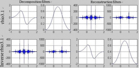
When the sign is set to negative, the waveform of the obtained wavelet “inverse rbio3.1 wavelet” is shown in Figure 1, and its filter bank can be expressed as:
$\left\{\begin{aligned} \tilde{g} &=\left\{\frac{\sqrt{2}}{8},-\frac{3 \sqrt{2}}{8}, \frac{3 \sqrt{2}}{8},-\frac{\sqrt{2}}{8}\right\} \\ g &=\left\{\frac{\sqrt{2}}{4}, \frac{3 \sqrt{2}}{4},-\frac{3 \sqrt{2}}{4},-\frac{\sqrt{2}}{4}\right\} \\ \tilde{h} &=\left\{-\frac{\sqrt{2}}{4}, \frac{3 \sqrt{2}}{4}, \frac{3 \sqrt{2}}{4},-\frac{\sqrt{2}}{4}\right\} \\ & h=\left\{\frac{\sqrt{2}}{8}, \frac{3 \sqrt{2}}{8}, \frac{3 \sqrt{2}}{8}, \frac{\sqrt{2}}{8}\right\} \end{aligned}\right.$
Figure 1. The waveform of the obtained wavelets
As shown in Figure 1, there were no substantial waveform difference between the two wavelets. The sign changes only led to the swap between reconstruction filter and decomposition filter. However, the swap may hinder the sequence construction of decomposition filters, and thus constrain wavelet application. Hence, the sign must be selected carefully in actual situation.
3.2 Parametric construction of odd-length biorthogonal wavelet
The parametric construction is possible if the high-pass decomposition filter sequence is of even length. If the filter sequence is odd in length, however, the biorthogonal wavelet might not be constructible in many cases. For example, the parametric construction method has no solution, when filter banks $\tilde{g}$↔h and g↔$\tilde{h}$ are of the same length. In some cases, the scale factor may have a fixed value.
If it is impossible to set up an odd-length biorthogonal wavelet, the solution is to adjust the sequence length, or change the scale factor and sign function.
Assuming that the low-pass decomposition filter sequence has a length of 3 and odd symmetry, the sequences of high-pass decomposition filters and low-pass reconstruction filters can be expressed as:
$\begin{aligned} \tilde{g} &=\left\{\tilde{g}_{0}, \tilde{g}_{1}, \tilde{g}_{2}\right\} \\ h_{k} &=(-1)^{k-1} \tilde{g}_{1-k} \\ h &=\left\{h_{-1}, h_{0}, h_{1}\right\} \end{aligned}$
In view of the odd symmetry, it is assumed that $\tilde{g}_{0}= \tilde{g}_{2}$. Since the sequence length is 3, the filter condition can be derived as:
$h=\left\{\frac{\sqrt{2}}{4}, \frac{\sqrt{2}}{2}, \frac{\sqrt{2}}{4}\right\}, \tilde{g}=\left\{\frac{\sqrt{2}}{4},-\frac{\sqrt{2}}{2}, \frac{\sqrt{2}}{4}\right\}$
It can be seen that the two low-pass filter sequences differ in length, and half of their total length cannot be odd. Then, the length of the low-pass decomposition filter sequence was adjusted to 5: $\tilde{h}=\left\{\tilde{h}_{-2}, \tilde{h}_{-1}, \tilde{h}_{0}, \tilde{h}_{1}, \tilde{h}_{2}\right\}$. Under the complete reconstruction condition, the following equations can be derived:
$\left\{\begin{aligned} \tilde{h}_{1}=\tilde{h}_{-1} & \tilde{h}_{2}=\tilde{h}_{-2} \\ \tilde{h}_{1}=\frac{\sqrt{2}}{4} & \tilde{h}_{0}+2 \tilde{h}_{2}=\frac{\sqrt{2}}{2} \\ 2 h_{1} \tilde{h}_{1}+h_{0} \tilde{h}_{0} &=1 \\ h_{1} \tilde{h}_{1}+h_{0} \tilde{h}_{2} &=0 \end{aligned}\right.\Rightarrow\left\{\begin{aligned} \tilde{h}_{0} &=\mp \frac{3 \sqrt{2}}{2 k} \\ \tilde{h}_{1} &=\frac{\sqrt{2}}{4} \\ \tilde{h}_{2} &=\pm \frac{\sqrt{2}}{4 k} \\ \tilde{h}_{0}+2 \tilde{h}_{2} &=\frac{\sqrt{2}}{2} \end{aligned}\right.$
At this point, the biorthogonal wavelet filter bank can be obtained as:
$h=\left\{\frac{\sqrt{2}}{4}, \frac{2 \sqrt{2}}{4}, \frac{\sqrt{2}}{4}\right\}$
$\tilde{g}=\left\{\frac{\sqrt{2}}{4},-\frac{2 \sqrt{2}}{4}, \frac{\sqrt{2}}{4}\right\}$
$\tilde{h}=\left\{-\frac{\sqrt{2}}{8}, \frac{\sqrt{2}}{4}, \frac{3 \sqrt{2}}{4}, \frac{\sqrt{2}}{4},-\frac{\sqrt{2}}{8}\right\}$
$g=\left\{\frac{\sqrt{2}}{8}, \frac{\sqrt{2}}{4},-\frac{3 \sqrt{2}}{4}, \frac{\sqrt{2}}{4}, \frac{\sqrt{2}}{8}\right\}$
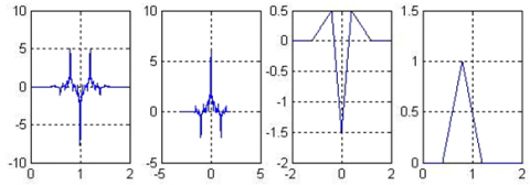
The biorthogonal wavelet obtained is bior2.2 wavelet, and its waveform is shown in Figure 2.
Figure 2. The waveform of the obtained wavelet
If the sequence of low-pass decomposition filters is 7 and evenly symmetric, then the sequences of high-pass decomposition filters and low-pass reconstruction filters can be expressed as:
$\tilde{g}=\left\{\tilde{g}_{-2}, \tilde{g}_{-1}, \tilde{g}_{0}, \tilde{g}_{1}, \tilde{g}_{2}, \tilde{g}_{3}, \tilde{g}_{4}\right\}$
$h=\left\{h_{-3}, h_{-2}, h_{-1}, h_{0}, h_{1}, h_{2}, h_{3}\right\}$
The scale factors $k_{1}, k_{2}, k_{3},\left(k_{i}>0 k_{i} \neq 1 \quad i=1,2,3\right)$ were introduced to adjust the proportionality within the sequence:
$\tilde{g}_{-2}=\tilde{g}_{4} \tilde{g}_{-1}=\tilde{g}_{3} \tilde{g}_{0}=\tilde{g}_{2} \tilde{g}_{3}=\pm k_{1} \tilde{g}_{4} \tilde{g}_{2}=\pm k_{2} \tilde{g}_{4} \tilde{g}_{1}=\pm k_{3} \tilde{g}_{4}$
For simplicity, it is assumed that $\tilde{g}_{4}=a a \neq 0 .$ Then, the sequence of high pass filters $\tilde{g}$ can be rewritten as:
$\tilde{g}=\left\{a, \pm k_{1} a, \pm k_{2} a, \pm k_{3} a, \pm k_{2} a, \pm k_{1} a, a\right\}$
The following can be derived from the relationship between $\tilde{g}$ and h:
$\begin{aligned} h=&\left\{a, \mp k_{1} a, \pm k_{2} a, \mp k_{3} a, \pm k_{2} a, \mp k_{1} a, a\right\} &=a\left\{1, \mp k_{1}, \pm k_{2}, \mp k_{3}, \pm k_{2}, \mp k_{1}, 1\right\} \end{aligned}$
Since the low-pass filter must meet the following conditions:
$\sum_{k} h_{2 k}=\sum_{k} h_{2 k+1}=\frac{1}{\sqrt{2}}$
Then, we have:
$\left\{\begin{array}{c}{a \pm k_{2} a=\frac{\sqrt{2}}{4}} \\ {\mp 2 k_{1} a \mp k_{3} a=\frac{\sqrt{2}}{2}}\end{array}\right.$ (6)
The length of low-pass decomposition filter sequence cannot be 7 and 3. The only viable length being examined is 5. Hence, the low-pass decomposition sequence can be defined as:
$\tilde{h}=\left\{\tilde{h}_{-2}, \tilde{h}_{-1}, \tilde{h}_{0}, \tilde{h}_{1}, \tilde{h}_{2}\right\}=\left\{\tilde{h}_{2}, \tilde{h}_{1}, \tilde{h}_{0}, \tilde{h}_{1}, \tilde{h}_{2}\right\}$
From the complete reconstruction condition and filter condition, we have:
$\left\{\begin{aligned} \tilde{h}_{1}=\frac{\sqrt{2}}{4} & \tilde{h}_{0}+2 \tilde{h}_{2}=\frac{\sqrt{2}}{2} \\ \mp 2 k_{1} \tilde{h}_{2} \pm \frac{\sqrt{2}}{2} k_{2} & \mp k_{3} \tilde{h}_{0}=\frac{1}{a} \\ \pm k_{1} \tilde{h}_{0} \pm k_{3} \tilde{h}_{2} &=\frac{\sqrt{2}}{4}\left(1 \pm k_{2}\right) \\ \tilde{h}_{2}=& \pm \frac{\sqrt{2}}{4 k_{1}} \end{aligned}\right.\Rightarrow\left\{\begin{array}{c}{\tilde{h}_{0}=\frac{\sqrt{2}}{2}\left(1 \mp \frac{1}{k_{1}}\right)} \\ {P R\text {Conditions }\left\{\begin{array}{c}{-\frac{\sqrt{2}}{2} \pm \frac{\sqrt{2}}{2} k_{2} \mp k_{3} \tilde{h}_{0}=\frac{1}{a}} \\ { \pm k_{1} \tilde{h}_{0} \pm k_{3} \tilde{h}_{2}=\frac{\sqrt{2}}{4}\left(1 \pm k_{2}\right)}\end{array}\right.} \\ {\tilde{h}_{2}=\pm \frac{\sqrt{2}}{4 k_{1}}}\end{array}\right.$ (7)
Combining equations (6) and (7), the filter bank of the constructed biorthogonal wavelet can be obtained, involving different scale factors and sign functions.
3.3 Instances on parametric construction of biorthogonal wavelet
The parametric construction of biorthogonal wavelet was illustrated with three instances.
Under the initial scale factor k1=3 and the sign function “-”, the sequences of high-pass decomposition filters and low-pass reconstruction filters can be derived by equations (6) and (7) as:
$h=\left\{-\frac{\sqrt{2}}{120},-\frac{\sqrt{2}}{40}, \frac{31 \sqrt{2}}{120}, \frac{11 \sqrt{2}}{20}, \frac{31 \sqrt{2}}{120},-\frac{\sqrt{2}}{40},-\frac{\sqrt{2}}{120}\right\}$
$\tilde{g}=\left\{-\frac{\sqrt{2}}{120}, \frac{\sqrt{2}}{40}, \frac{31 \sqrt{2}}{120},-\frac{11 \sqrt{2}}{20}, \frac{31 \sqrt{2}}{120}, \frac{\sqrt{2}}{40},-\frac{\sqrt{2}}{120}\right\}$
The obtained biorthogonal wavelet is denoted as wavelet zqwo6e3.
Under the initial scale factor k1=5 and the sign function “+”, the biorthogonal wavelet filter bank can be obtained as:
$\tilde{h}=\left\{\frac{\sqrt{2}}{20}, \frac{\sqrt{2}}{4}, \frac{2 \sqrt{2}}{5}, \frac{\sqrt{2}}{4}, \frac{\sqrt{2}}{20}\right\}$
$g=\left\{-\frac{\sqrt{2}}{20}, \frac{\sqrt{2}}{4},-\frac{2 \sqrt{2}}{5}, \frac{\sqrt{2}}{4},-\frac{\sqrt{2}}{20}\right\}$
$h=\left\{\frac{7 \sqrt{2}}{120},-\frac{7 \sqrt{2}}{24}, \frac{23 \sqrt{2}}{120}, \frac{13 \sqrt{2}}{12}, \frac{23 \sqrt{2}}{120},-\frac{7 \sqrt{2}}{24}, \frac{7 \sqrt{2}}{120}\right\}$
$\tilde{g}=\left\{\frac{7 \sqrt{2}}{120}, \frac{7 \sqrt{2}}{24}, \frac{23 \sqrt{2}}{120},-\frac{13 \sqrt{2}}{12}, \frac{23 \sqrt{2}}{120}, \frac{7 \sqrt{2}}{24}, \frac{7 \sqrt{2}}{120}\right\}$
The obtained biorthogonal wavelet is denoted as wavelet zqwo6e5.
Under the initial scale factor k1=5 and the sign function “-”, the biorthogonal wavelet filter bank can be obtained as:
$\begin{aligned} \tilde{h} &=\left\{-\frac{\sqrt{2}}{20}, \frac{\sqrt{2}}{4}, \frac{3 \sqrt{2}}{5}, \frac{\sqrt{2}}{4},-\frac{\sqrt{2}}{20}\right\} \\ g &=\left\{\frac{\sqrt{2}}{20}, \frac{\sqrt{2}}{4},-\frac{3 \sqrt{2}}{5}, \frac{\sqrt{2}}{4}, \frac{\sqrt{2}}{20}\right\} \end{aligned}$
$h=\left\{-\frac{3 \sqrt{2}}{280},-\frac{15 \sqrt{2}}{280}, \frac{73 \sqrt{2}}{280}, \frac{170 \sqrt{2}}{280}, \frac{73 \sqrt{2}}{280},-\frac{15 \sqrt{2}}{280},-\frac{3 \sqrt{2}}{280}\right\}$
$\tilde{g}=\left\{-\frac{3 \sqrt{2}}{280}, \frac{15 \sqrt{2}}{280}, \frac{73 \sqrt{2}}{280},-\frac{170 \sqrt{2}}{280}, \frac{73 \sqrt{2}}{280}, \frac{15 \sqrt{2}}{280},-\frac{3 \sqrt{2}}{280}\right\}$
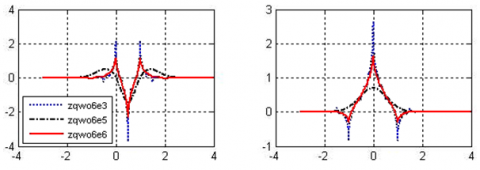
The waveforms of the decomposition filters of the above wavelets are shown in Figure 3.
Figure 3. The waveform of the decomposition filters of the obtained wavelets
The vanishing moment of wavelet construction was not explained in the three instances. The order of vanishing moment of the biorthogonal wavelet can be obtained by limiting the scale factor to the first pd-order derivative of zero. If the first pd-order derivative of the decomposition scale function and the first pr-order derivative of the reconstruction scale function are both zero, then the constructed biorthogonal wavelet must have the vanishing moment of orders pd and pr respectively in decomposition and reconstruction.
Due to the waveform difference of wavelets, each wavelet has its unique symmetry, regularity and support tightness. Besides, the wavelet basis varies with the signal or image to be processed. To verify the denoising effect of the constructed wavelet, six biorthogonal wavelets (bior5.5, bior2.6, bior4.4, zjhwo6e3, zjhwo6e5 and zjhwo6e6) were cited for threshold denoising of two noisy images. All of them are evenly symmetric at zero point.
The two images are “Lifting body”, a distant view of a plane in the air, and “Lena”, a close shot of a beautiful girl. The latter image has much more details than the former. To facilitate recognition and analysis, the original images were enhanced to eliminate irrelevant information, improve image effect and highlight image features.
Then, the simulation was conducted on Matlab, using global threshold denoising (GTD) and self-adaptive hierarchical threshold denoising (SAHTD). The decomposition scale was set to 2~5, the signal-to-noise ratios (SNRs) were initialized as 15 and 20, respectively, and the hard thresholding was selected according to the ddencmp function in the Matlab.
The denoising effects of the two methods on Lifting Body are compared in Table 1. The comparison shows that, using the GTD, the SNRs of all wavelets decreased with the growth in decomposition scale, owing to the accidental deletion of image details. The denoising effect of wavelet bior5.5 decreased faster than that of any other wavelet, indicating that this wavelet performs the worst in retaining the low-frequency approximation information.
By contrast, the image details were completely preserved by the SAHTD, while all noises were removed, pushing up the image SNR. This is attributable to the modification of all scales by this method. The SNR of the denoised image increased with the decomposition scale, before the latter surpassed 4.
Table 1. Comparison of the denoising effects on Lifting Body
|
Initial condition Wavelet |
Initial SNR =15 |
Initial SNR =20 |
||||||
|
N=2 |
N=3 |
N=4 |
N=5 |
N=2 |
N=3 |
N=4 |
N=5 |
|
|
GTD results |
||||||||
|
bior5.5 |
24.59 |
24.2 |
22.5 |
21.63 |
26.98 |
25.26 |
24.17 |
23.77 |
|
bior2.6 |
24.66 |
25.17 |
24.74 |
24.45 |
27.24 |
27.07 |
26.75 |
26.75 |
|
bior2.2 |
24.47 |
25.01 |
24.76 |
24.47 |
26.99 |
26.77 |
26.55 |
26.4 |
|
zjhwo6e12 |
24.62 |
25.2 |
24.8 |
24.51 |
27.24 |
27.05 |
26.88 |
26.76 |
|
zjhwo6e14 |
24.61 |
25.14 |
24.79 |
24.51 |
27.23 |
27.11 |
26.87 |
26.73 |
|
zjhwo6e16 |
24.59 |
25.12 |
24.77 |
24.48 |
27.22 |
27.1 |
26.86 |
26.73 |
|
SAHTD results |
||||||||
|
bior5.5 |
24.63 |
25.72 |
25.68 |
25.7 |
27.4 |
27.6 |
27.67 |
27.63 |
|
bior2.6 |
24.28 |
24.78 |
24.67 |
24.68 |
27.51 |
27.77 |
27.86 |
27.83 |
|
bior2.2 |
23.8 |
23.914 |
23.912 |
23.911 |
27.24 |
27.28 |
27.27 |
27.27 |
|
zqwo6e12 |
24.13 |
24.59 |
24.55 |
24.51 |
27.4 |
27.69 |
27.74 |
27.66 |
|
zqwo6e14 |
24.15 |
24.64 |
24.56 |
24.54 |
27.42 |
27.71 |
27.75 |
27.71 |
|
zqwo6e16 |
24.14 |
24.61 |
24.54 |
24.54 |
27.43 |
27.71 |
27.73 |
27.73 |
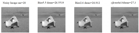
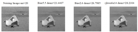
The denoising effects of the GTD and the SAHTD on Lifting Body are presented in Figures 4 and 5, respectively. The initial SNR was 20 and the decomposition scale was 5. As shown in the two figures, the SAHTD outperformed the GTD in the SNR and the preservation of image details. The contrast is particularly obvious on wavelet bior5.5: the GTD denoised image was completely blurred.
Figure 4. The denoising effect of the GTD on Lifting Body (SNR=20)
Figure 5. The denoising effect of the SAHTD on Lifting Body (SNR=20)
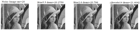
The denoising effects of the two methods on Lena are compared in Table 2, where the decomposition scale ranges between 2 and 5 and the initial SNRs were 15 and 20. The comparison shows that the SAHTD outshined the GTD in denoising such a complex image with rich details, whichever the condition. The rich details make it easy to delete details by accident, and hard to increase the SNR. Despite its acceptable performance on Lifting Body, a simple noisy image, the GTD performed poorly on Lena, and even reduced the SNR in some cases.
The denoising effects of the GTD and the SAHTD on Lena are plotted as Figures 6 and 7, respectively. The initial SNR was 20 and the decomposition scale was 5. As shown in the two figures, using the GTD, the SNR of bior5.5 plummeted, while the image quality of the other wavelets improved slightly. In the images denoised by the GTD, the edges blurred to different degrees, and the background was basically indiscernible. By contrast, all wavelet except bior5.5 greatly enhanced the image quality by the SAHTD. The denoised images had little noise, clear edges and well-preserved backgrounds.
Table 2. Comparison of the denoising effects on Lena
|
Initial condition Wavelet |
Initial SNR=15 |
Initial SNR=20 |
||||||
|
N=2 |
N=3 |
N=4 |
N=5 |
N=2 |
N=3 |
N=4 |
N=5 |
|
|
GTD results |
||||||||
|
bior5.5 |
19.54 |
18.78 |
17.57 |
17.09 |
20.593 |
19.493 |
18.578 |
18.3 |
|
bior2.6 |
19.67 |
19.48 |
19.18 |
19.16 |
20.868 |
20.506 |
20.314 |
20.219 |
|
bior2.2 |
19.48 |
19.15 |
18.86 |
18.77 |
20.72 |
20.28 |
20.09 |
20.05 |
|
zjhwo6e12 |
19.63 |
19.48 |
19.16 |
19.13 |
20.877 |
20.532 |
20.316 |
20.213 |
|
zjhwo6e14 |
19.631 |
19.49 |
19.185 |
19.16 |
20.859 |
20.517 |
20.322 |
20.222 |
|
zjhwo6e16 |
19.641 |
19.51 |
19.186 |
19.15 |
20.863 |
20.521 |
20.303 |
20.217 |
|
SAHTD results |
||||||||
|
bior5.5 |
19.84 |
19.8 |
19.7 |
19.75 |
21.12 |
20.88 |
20.83 |
20.82 |
|
bior2.6 |
20.0 |
19.935 |
19.95 |
19.93 |
21.255 |
21.3 |
21.26 |
21.275 |
|
bior2.2 |
19.78 |
19.727 |
19.721 |
19.72 |
21.15 |
21.12 |
21.11 |
21.11 |
|
zjhwo6e12 |
19.93 |
19.87 |
19.898 |
19.89 |
21.21 |
21.24 |
21.22 |
21.241 |
|
zjhwo6e14 |
19.96 |
19.88 |
19.904 |
19.86 |
21.22 |
21.27 |
21.23 |
21.266 |
|
zjhwo6e16 |
19.946 |
19.867 |
19.905 |
19.87 |
21.221 |
21.26 |
21.234 |
21.25 |
Figure 6. The denoising effect of the GTD on Lena (SNR=20)
Figure 7. The denoising effect of the SAHTD on Lena (SNR=20)
he simulation verifies that the three wavelets constructed by our method can denoise images with different complexities and noise levels, using large decomposition scales. Comparing the SNRs of the three wavelets, it is concluded that the denoising of simple images does not necessarily lead to a large vanishing moment of wavelets; the wavelet’s denoising effect increases with the vanishing moment for complex images; the SAHTD depends less on wavelet features, applies to more types of images and preserves more details at high decomposition scale than the GTD.
Inspired by wavelet threshold denoising, this paper proposes a parametric construction method for biorthogonal wavelet of even symmetry at the zero point, using the sequence length of (13-3) and the 2nd/4th/6th-order vanishing moments. The constructed wavelets were simulated on two noisy images with the GTD and SAHTD. The simulation results show that the constructed wavelets can remove noises from the original image while preserving most image details. Combined with the SAHTD, the proposed wavelet construction method can greatly improve image quality and the SNR. The future research will explore the wavelet threshold denoising of images containing different types of noises, and evaluate the complexity of the denoising effect.
The author was endowed by Water Conservancy Science and Technology Plan Project of Shaanxi Province(2019slkj-19) and Industry University Research Project in Yulin city (2015CXY-21).
[1] Wang, X., Ou, X., Chen, B.W., Kim, M. (2019). Image denoising based on improved wavelet threshold function for wireless camera networks and transmissions. International Journal of Distributed Sensor Networks, 2015(2): 23. https://doi.org/10.1155/2015/670216
[2] Ruan, C., Zhao, D., Jia, W., Chen, C., Chen, Y., Liu, X. (2015). A new image denoising method by combining WT with ICA. Mathematical Problems in Engineering, 2015: 1-10. https://doi.org/10.1155/2015/582640
[3] Zhao, H.H., Lopez, J.F., Martinez, A., Qiao, Z.J. (2013). SAR image denoising based on wavelet packet and median filter. Applied Mechanics and Materials, 333-335: 916-919. https://doi.org/10.4028/www.scientific.net/AMM.333-335.916
[4] Xu, D., Sun, L., Luo, J., Liu, Z. (2013). Analysis and denoising of hyperspectral remote sensing image in the curvelet domain. Mathematical Problems in Engineering, 2013. https://doi.org/10.1155/2013/751716
[5] Wang, Y., Lei, F., Fu, G.J. (2013). Adaptive denoising algorithms based on wavelet for pool underwater image. Applied Mechanics and Materials, 333-335: 1024-1029. https://doi.org/10.4028/www.scientific.net/AMM.333-335.1024
[6] Kaur R., Kaur, J. (2013). Comparative analysis of speckle reduction techniques in ultrasound images. International Journal of Computer Applications in Engineering Sciences, 3(1): 26-28. https://doi.org/10.1.1.310.9522
[7] Tian, J., Li, Y., Wang, H. (2012). An image filtering algorithm based on translation invariance wavelet transform. Journal of Projectiles, Rockets, Missiles and Guidance, 32: 140-142.
[8] Chen, G., Zhu, W.P. (2012). Signal denoising using neighbouring dual-tree complex wavelet coefficients. IET Signal Processing, 6: 143-147.
[9] Al-geelani, N.A., Piah, M.A.M. (2012). Identification and extraction of surface discharge acoustic emission signals using wavelet neural network. International Journal of Computer and Electrical Engineering, 4(4): 471-474.
[10] Mahajan, A., Birajdar, G. (2011). Analysis of blind separation of noisy mixed images based on wavelet thresholding and independent component analysis. International Journal of Engineering and Technology, 3(5): 560-564.
[11] Li, Q., Ge, P., Feng, H.J., Xu, Z.H. (2011). Image displacement detection under low illumination using joint transform correlator with wavelet denoising. Applied Mechanics and Materials, 128-129: 602-606. https://doi.org/10.4028/www.scientific.net/AMM.128-129.602
[12] Bhutada, G.G., Anand, R.S., Saxena, S.C. (2011). Image enhancement by wavelet-based thresholding neural network with adaptive learning rate. IET Image Processing, 5(7): 573-582. https://doi.org/10.1049/iet-ipr.2010.0014
[13] Hu, Y., Zhang, Y., Xiong, C.J., Chen, X.B. (2010). Denoising method with wavelet shrinkage adaptive thresholding and wiener filter. Journal of University of Science and Technology Liaoning, 33: 539-542.
[14] Shi, H.B., Ma, S.L., Han, X. (2007). A new method based on the wavelet transformation of image denoising. Journal of Jilin University, 45: 607-610.
[15] Yang, F., Zhang, Y., Wang, Z., Yang, Q. (2006). Application of wavelet transform-based wiener filtering method to reduce additive noise in apple image. Transactions of the Chinese Society of Agricultural Machinery, 37: 130-133.
[16] Chan, R.H., Chan, T.F., Shen, L., Shen, Z. (2003). Wavelet algorithms for high-resolution image reconstruction. SIAM Journal on Scientific Computing, 24: 1408-1425.