Reliability Model and State Probabilities of Electrical System, Subject to Multiple Competing Failure Processes

In power systems, components often experience gradual degradation rather than sudden failure. Their operational status can be described through a finite set of degradation states. For instance, an Oil Circuit Breaker (OCB) deteriorates progressively due to two main degradation mechanisms: the aging of the insulating oil and the wear of the electrical contacts. These degradations are further influenced by random shocks caused by the mechanical and electrical stresses encountered during fault isolation, such as short circuits. The failure of the system occurs if any one of these three independent degradation processes surpasses its respective critical threshold.

A large amount of research has occurred on degraded systems and their reliability, as well as inspection and maintenance.

Li and Pham [1] developed a reliability model of a degraded system subject to multiple competing failure processes. Zuo et al. [2] developed a mixture framework in which the population is partitioned into two distinct cohorts: one cohort experiences gradual degradation, while the other is prone to sudden, catastrophic failure. Finkelstein and Marais identify two fundamental shock paradigms: cumulative shocks, where damage accumulates incrementally over time, and extreme shocks, where a single, unusually severe event precipitates immediate failure [3]. Building on this, Cha and Finkelstein propose a combined shock model that integrates both the additive nature of cumulative damage and the abrupt impact of extreme shocks, offering a unified perspective on dual-mode failure mechanisms [4].

Klutke and Yang [5] analyzed the availability of systems under maintenance, considering the combined influence of degradation and random shock events. In their model, shocks follow a Poisson process, and their magnitudes are treated as independent and identically distributed random variables. A brief overview of failure mechanism in Oil Circuit Breakers (OCB’s) appears in section 2, to justify the importance of degradation considerations [6]. Regarding its design and its function, the OCB is a component of choice to highlight both reliability modeling and reliability data analysis of a degraded system, as presented in section 3 [7]. 

Building on this foundation, other studies have further advanced the modelling of degraded systems and circuit breakers. Iberraken et al. [8] and Medjoudj et al. [9] proposed a preventive maintenance model integrating oil aging, contact wear, and random shocks, optimized to improve OCB availability through technical and organizational means. Their work refines this framework by quantifying the relative impact of shocks versus continuous degradation on breaker performance [10].

Xie et al. [11] applied a two-stage Wiener process model to characterize degradation of a smart (low-voltage) circuit breaker control circuit. Their results reveal a turning point at almost 155,000 hours and a predicted lifetime of 178,000 hours (20 years), providing a strong precedent for staged stochastic modeling. It brings insight into multi-phase degradation patterns that inform OCB modeling. Ranganathan Sakthivel Gundala Vijayalakshmi proposed a method to determine the reliability of complex systems using a Bayesian network (BN). This probabilistic graphical model represents knowledge about an uncertain domain, where each component is modeled as a random variable and each edge corresponds to a conditional probability. Their approach applies the Bayesian network to estimate the reliability of a multistate consecutive k-out-of-n: F system [12].

Wahyudi and Wicaksono [13] proposed a reliability device model simulation as an effective learning media to enhance students’ understanding and technical skills in designing reliability engineering systems (RES). Their model offers options for series, parallel, and combined series-parallel systems. Using Accelerated Life Testing (ALT) analyzed through statistical methods, they estimated system lifetimes under normal conditions.

This paper proposes a method for generating system states under multiple failure processes. It is based on a real case study involving OCBs affected by contact wear and random shocks. A second scenario, discussed in Sections 4 and 5, considers OCBs exposed to two degradation processes contact wear and insulating oil aging along with random shocks. Detailed results for both cases are provided.

Today's electrical power grid has a significant number of highly efficient OCB’s installed.  Design and function of OCB’s offer the possibility of implementing both degradation and shocks processes, namely slow degradations (contact wear and liquid dielectric aging) and random shocks. Replacement of the OCB is unrealistic and prohibitive considering the long life duration of the component (about 30 years) and its cost. This component corresponds to a set of technologies with a specific congestion, subject to multitude changes during this period.

3.1 Shock analysis

Random shocks happen intermittently over time, inflicting incremental damage to the system that accumulates and progressively degrades its integrity. Failure occurs once the accumulated damage surpasses a critical threshold. For reliability modeling, the values of probability distribution parameters are needed.  In the OCB case, a power utility would face difficulty and expense in carrying out any experimental test. Consequently, utilities prefer construction of any model using experience data [19].

3.1.1 Shock modeling

The probability that the device survives to shocks is:

${{\bar{P}}_{k}};k=0,1,2,\ldots$

where $1={{\bar{P}}_{0}}\ge \overline{{{P}_{1}}}\ge \overline{{{P}_{2}}}$. Let N={N(t): t≥0} representing the occurrence of shocks that is modeled as a counting process. The likelihood that the device remains operational after time t can be expressed as:

$\bar{H}\left( t \right)=\underset{k=0}{\overset{\infty }{\mathop \sum }}\,P\left[ N\left( t \right)=k \right].\overline{{{P}_{k}}}$    (1)

The shock model described in Eq. (1) is particularly relevant for reliability engineers aiming to analyze the aging behavior of system components, especially when data regarding the intensity and frequency of shocks is available.

3.1.2 Case study

Shocks data exists for OCB operations, collected from 2009 to 2024 - 15 years of continuous system operation at Sonelgaz Company of Bejaia city district (Algeria). The annual number of shocks, treated as a random variable, is modeled using either the exponential $E\left( \lambda  \right)~$or Weibull $W\left( \beta ,\eta  \right)$ distributions as often used for data analysis in electrical systems wo commonly adopted models in the reliability assessment of electrical systems. The parameters of these distributions can be estimated through maximum likelihood estimation (MLE) and probability plotting. While MLE typically yields more accurate estimates, probability plotting serves as a useful visual tool to assess the goodness-of-fit [20, 21]. Based on the available data and employing the R statistical environment, we estimated the distribution parameters for Weibull and exponential laws, as represented in the Table 1. To validate the most appropriate distribution, we applied the Kolmogorov-Smirnov (KS) test. The full procedure follows the methodology outlined in references [22, 23] and summarized as follows.

Table 1. Results of (KS) test of shock arrivals

Based on the Kolmogorov-Smirnov test, the results given in Table 1 show the value of  is lower than ${{d}_{\left( n,0.05 \right)}}$ [24].

In a study of shock classifications, Mollar and Oney [25] established for the distribution function ${{F}_{j}}$ describing the damage inflicted by the ${{j}^{th}}$ shock, two alternative formulations for the sequence $\left\{ \overline{{{P}_{k}}} \right\}$, depending on the shock - for the cumulative shock model, $\overline{{{P}_{k}}}={{F}_{1}}*{{F}_{2}}*...*{{F}_{k}}\left( s \right)$ (convolution product), and for the extreme shock model, $\overline{{{P}_{k}}}=\mathop{\prod }_{j=1}^{k}{{F}_{j}}\left( s \right)$ with s a prefixed threshold value.

For the case study treated in this paper, N(t) is modeled by a non-homogeneous Poisson process (NHPP) and is characterized by a Poisson distribution defined by a specific parameter representing the mean value, referred to as the rate $\lambda \left( t \right)=\frac{d\Lambda \left( t \right)}{dt}$, Both are specified on the interval from zero to infinity. Under these conditions, the shock model (1) can be expressed as follows:

$\bar{H}\left( t \right)=\underset{k=1}{\overset{\infty }{\mathop \sum }}\,\frac{{{\Lambda }^{k}}\left( t \right)}{k!}{{e}^{-\Lambda \left( t \right)}}\,\overline{{{P}_{k}}}$    (2)

5.1 Degraded system subject to two competing failure processes

The OCB is subject to two failure mechanisms (noted case 1) defined by:

-The increasing degradation process Y₁(t) representing the wear of the circuit breaker contacts, where the failure probability function of the contacts is given by Eq. (3).

-The cumulative shocks damages is given by:

$D\left( t \right)=\underset{i=1}{\overset{N\left( t \right)}{\mathop \sum }}\,{{X}_{i}}$.

These two processes consist of random variables that are mutually independent and share the same probability distribution, with $\lambda \left( t \right)=\frac{{{\beta }_{2}}\cdot {{t}^{{{\beta }_{2}}-1}}}{{{\eta }_{2}}^{{{\beta }_{2}}}}$.

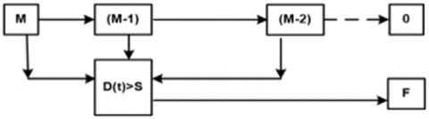
The diagram of states of this system is presented in the Figure 1.

1.png

Figure 1. Degradation and failure States diagram of the equipment (Case 1)

The system operates through degradation states labeled M, (M – 1)…1, with state representing failure, and F corresponding to catastrophic failure.  During its operation, the OCB may gradually move from state i to state $i-1$ due to progressive deterioration, or it may directly fail by transitioning to the failure state F because of random shocks. Let's ${{W}_{i}}$ be a degradation state level where the system resides temporarily i, ${{G}_{1}}$ the degradation threshold, or the failure state 0 and S the critical threshold for cumulative shocks. The system enters the catastrophic failure state F when this critical limit is exceeded. State M is considered the initial state, and the system is assumed to be as good as new at this point. The probabilities of the system being in states M, $0<i<M$, 0 and  are given respectively:

${{P}_{M}}\left( t \right)=P\left[ {{Y}_{1}}\left( t \right)<{{W}_{M}},D\left( t \right)=\underset{i=1}{\overset{N\left( t \right)}{\mathop \sum }}\,{{X}_{i}}\le S \right]$    (5)

${{P}_{i}}\left( t \right)=P\left[ {{W}_{i}}<{{Y}_{1}}\left( t \right)<{{W}_{i+1}},D\left( t \right)=\underset{i=1}{\overset{N\left( t \right)}{\mathop \sum }}\,{{X}_{i}}\le S \right]$    (6)

${{P}_{0}}\left( t \right)=P\left[ {{Y}_{1}}\left( t \right)>{{G}_{1}},D\left( t \right)=\underset{i=1}{\overset{N\left( t \right)}{\mathop \sum }}\,{{X}_{i}}\le S \right]$    (7)

${{P}_{F}}\left( t \right)=P\left[ {{Y}_{1}}\left( t \right)<{{G}_{1}},D\left( t \right)=\underset{i=1}{\overset{N\left( t \right)}{\mathop \sum }}\,{{X}_{i}}>S \right]$    (8)

The development of Eqs. (5)-(8), using explanations of functions and parameters, results in new expressions of the above probabilities as follows:

${{P}_{2}}\left( t \right)=\left[ 1-\text{exp}\left( -{{\left[ \frac{{{W}_{1}}}{{{W}_{0}}} \right]}^{{{\beta }_{1}}}}{{\left[ \frac{t}{{{t}_{0}}} \right]}^{\frac{{{\beta }_{1}}}{n-b{{T}_{1}}}{{e}^{\frac{{{\beta }_{1}}B\text{T}}{n-b{{T}_{1}}}}}}} \right) \right]$ $\times \left[ {{e}^{-\lambda \left( t \right)}}\underset{j=0}{\overset{\infty }{\mathop \sum }}\,\left( \frac{{{\left( \lambda \left( t \right) \right)}^{j}}}{j!} \right){{F}_{x}}^{\left( j \right)}\left( S \right) \right]$    (9)

The OCB is considered to have failed once the deterioration process surpasses the limit G₁, or the cumulative shock damage crosses some threshold S. The application is done for the case of two degradation states and Figure 1 could be exploited when considering M = 2. The threshold values for each state correspond to the relative wear of the OCB contacts and they are given as follows: W1 = 0.45, G1 = 1. However, the threshold of the cumulative shocks S = 100, representing the number of the strong solicitations of the circuit breaker. The Weibull parameter is given by: ${{\beta }_{1}}=2,009771$.

${{P}_{1}}\left( t \right)=\left[ \left[ 1-\text{exp}\left( -{{\left[ \frac{{{G}_{1}}}{{{W}_{0}}} \right]}^{{{\beta }_{1}}}}{{\left[ \frac{t}{{{t}_{0}}} \right]}^{\frac{{{\beta }_{1}}}{n-b{{T}_{1}}}{{e}^{\frac{{{\beta }_{1}}B\text{T}}{n-b{{T}_{1}}}}}}} \right) \right]-\left[ 1-\text{exp}\left( -{{\left[ \frac{{{W}_{1}}}{{{W}_{0}}} \right]}^{{{\beta }_{1}}}}{{\left[ \frac{t}{{{t}_{0}}} \right]}^{\frac{{{\beta }_{1}}}{n-b{{T}_{1}}}{{e}^{\frac{{{\beta }_{1}}B\text{T}}{n-b{{T}_{1}}}}}}} \right) \right] \right]\times \left[ {{e}^{-\lambda \left( t \right)}}\underset{j=0}{\overset{\infty }{\mathop \sum }}\,\left( \frac{{{\left( \lambda \left( t \right) \right)}^{j}}}{j!} \right){{F}_{x}}^{\left( j \right)}\left( S \right) \right]$    (10)

${{P}_{0}}\left( t \right)=\exp \left( -{{\left[ \frac{{{G}_{1}}}{{{W}_{0}}} \right]}^{{{\beta }_{1}}}}{{\left[ \frac{t}{{{t}_{0}}} \right]}^{\frac{{{\beta }_{1}}}{n-b{{T}_{1}}}{{e}^{\frac{{{\beta }_{1}}B{{T}_{{}}}}{n-b{{T}_{1}}}}}}} \right)$$\times \left[ {{e}^{-\lambda \left( t \right)}}\mathop{\sum }_{j=0}^{\infty }\left( \frac{{{\left( \lambda \left( t \right) \right)}^{j}}}{j!} \right){{F}_{x}}^{\left( j \right)}\left( S \right) \right]$    (11)

${{P}_{F}}\left( t \right)=\left[ 1-\exp \left( -{{\left[ \frac{{{G}_{1}}}{{{W}_{0}}} \right]}^{{{\beta }_{1}}}}{{\left[ \frac{t}{{{t}_{0}}} \right]}^{\frac{{{\beta }_{1}}}{n-b{{T}_{1}}}{{e}^{\frac{{{\beta }_{1}}BT}{n-b{{T}_{1}}}}}}} \right) \right]$$\times \left[ 1-{{e}^{-\lambda \left( t \right)}}\mathop{\sum }_{j=0}^{\infty }\left( \frac{{{\left( \lambda \left( t \right) \right)}^{j}}}{j!} \right){{F}_{x}}^{\left( j \right)}\left( S \right) \right]~$    (12)

The reliability is given by:

${{R}_{M}}\left( t \right)=P\left[ state\ge 1 \right]=\underset{i=1}{\overset{M}{\mathop \sum }}\,{{P}_{i}}\left( t \right)~$    (13)

2.png

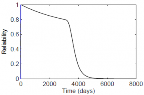
Figure 2. Reliability evaluation

The reliability analysis of the Oil Circuit Breaker (OCB) under a single degradation process, as depicted in Figure 2, reveals that the system is projected to fail after approximately 14 years if no maintenance or repair is performed. This "unmaintained" lifespan serves as a baseline for the inherent durability of the OCB under its initial design and operating conditions.

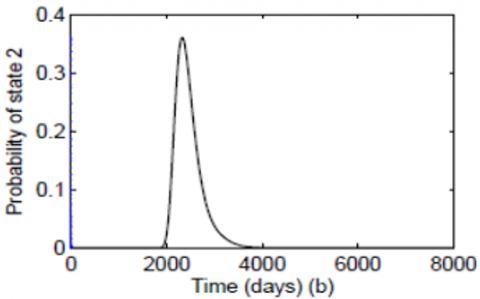
The failure in this context encompasses the OCB reaching a state where it can no longer reliably or safely fulfill its intended function. This may include various degraded states culminating in catastrophic failure. The probability of catastrophic failure (state F) reaches a threshold value of 0.2 at 9 years, indicating a significant risk of complete breakdown at this point. The reliability function is explicitly governed by a random shock process, suggesting that while continuous degradation is ongoing, sharp declines in reliability or even immediate failures are primarily triggered by sudden, unpredictable events. These shocks may include transient overvoltages, short-circuit currents, environmental extremes, or mechanical stresses, all of which can precipitate failure in a system already weakened by gradual wear.

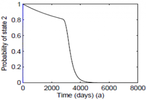
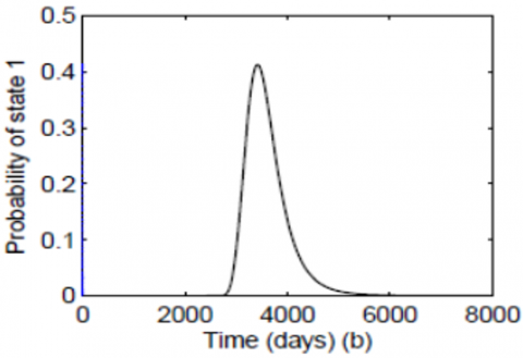
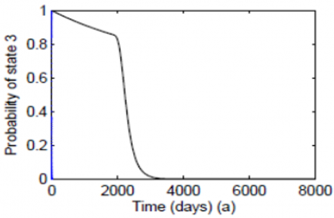
Comparing the reliability evolution to the initial state probabilities (Figure 3(a)), it is evident that the system starts with a high probability of being in a healthy state. Over time, this probability diminishes, and the likelihood of being in degraded or failed states increases, confirming that degradation is the dominant long-term trend. This underscores the time-dependent and dynamic nature of OCB health.

3a.png

3b.png

3c.png

3d.png

Figure 3. Degradation states and failure probabilities

5.2 Degraded system subject to three competing failure processes

To the development given in sub-section (5.1), an additional deterioration process, labeled Y₂(t) is introduced to represent the effects of aging of insulating oil of a swichgear (noted case 2). As illustrated in the diagram (Figure 4), we consider that each degradation process (oil aging, contact wear) evolves independently, but once either reaches a certain degradation threshold, it can trigger elementary shocks. When the cumulative effect of these shocks exceeds a critical level, a major shock occurs, leading to system failure. This interaction is captured through the shock modeling framework, which indirectly reflects the coupling effect in the failure mechanism.

4.png

Figure 4. Degradation and failure States diagram of equipment subjet two degradation processes and shocks

For the first deterioration process, two degradation levels are taken into account ($M=2$), while the second deterioration process includes three distinct degradation levels ($M=3$).  System failure occurs if the degradation level or the shock damage reaches its respective failure limit ${{y}_{i}}\left( t \right)$exceeds a certain limit ${{G}_{i}},i=1,2$, alternatively, failure occurs when the cumulative impact of shocks attains its designated threshold S.

The state spaces associated to degradation process 1 and degradation process 2 are, respectively, ${{\Omega }_{1}}=\left\{ {{2}_{1}},{{1}_{1}},{{0}_{1}} \right\}~$and  ${{\Omega }_{2}}=\left\{ {{3}_{2}},{{2}_{2}},{{1}_{2}},{{0}_{2}} \right\}$. Subsequently, the set of possible states of the system is characterized as ${{\Omega }_{u}}=\left\{ 3,2,1,0,F \right\}$.

Building on the work of Pham [3], we propose a methodology to establish a relationship between the combination of all possible states resulting from the interaction of individual degradation processes $\Omega $ and the degradation state spaces $\left\{ {{\Omega }_{1}},{{\Omega }_{2}} \right\}$. This is done under the assumption that the system has not yet reached catastrophic failure; state F is temporarily excluded from the analysis. The interaction between the degradation processes is defined through a mapping function f, expressed as follows: $f:C={{\Omega }_{1}}x{{\Omega }_{2}}\to \Omega =\left\{ 3,2,1,\left. 0 \right\} \right.$, where C denote a Cartesian product that forms the domain of the input space. The matrix H presented below represents the output space, which contains M + 1 elements. Each of these elements corresponds to an element in the input space domain via the mapping defined by the function f.

$H=\overset{\begin{matrix}{} & {{0}_{2}} & {{1}_{2}} & {{2}_{2}} & {{3}_{2}}  \\\end{matrix}}{\mathop{\begin{matrix}{{0}_{1}}  \\{{1}_{1}}  \\{{2}_{1}}  \\\end{matrix}\left[ \begin{matrix} x & 0 & 0 & 0  \\ 0 & 0 & 2 & 2  \\ 0 & 1 & 2 & 3  \\\end{matrix} \right]}}\,$

The mapping function f and the construction of the matrix H are based on a bi-dimensional degradation process, where: the rows represent degradation states of electrical contacts, and the columns represent degradation states of the insulating oil. Each element H_i.j corresponds to a combined degradation level of the system, derived from expert judgment and field feedback, following the modeling approach proposed by Whang, Zhou, Wang, and Pham in the context of multi-state system reliability. The elements of H represent $f\left( {{i}_{1}},{{j}_{2}} \right)=k$ where ${{i}_{1}}\in {{\Omega }_{1}},{{j}_{2}}\in {{\Omega }_{2}}$  and $k\in \Omega $. Every element located in the first row and the first column is equal to zero, except that denoted by x because a degraded condition is triggered when one of the degradation components attains its maximum state ${{0}_{i}},i=1,2$. Also, $f\left( {{M}_{1}},{{M}_{2}} \right)=M=3$ because at the start, the system is assumed to be in flawless condition. The overall system state is determined by the combination of the states from each degradation process. The equivalence classes for degrading states and failure state can be listed as follows:

${{R}_{0}}=\left\{ \left( {{0}_{2}},{{1}_{1}} \right),\left( {{0}_{2}},{{2}_{1}} \right),\left( {{1}_{2}},{{0}_{1}} \right),\left( {{2}_{2}},{{0}_{1}} \right),\left( {{3}_{2}},{{0}_{1}} \right),\left( {{1}_{2}},{{1}_{1}} \right) \right\}$, ${{R}_{1}}=\left\{ \left( {{1}_{2}},{{2}_{1}} \right) \right\},~~{{R}_{2}}=\left\{ \left( {{2}_{2}},{{1}_{1}} \right),\left( {{2}_{2}},{{2}_{1}} \right),\left( {{3}_{2}},{{1}_{1}} \right) \right\}$,

${{R}_{3}}=\left\{ \left( {{3}_{2}},{{2}_{1}} \right) \right\}$ And $R=\underset{i=0}{\overset{3}{\mathop \sum }}\,{{R}_{i}}$.

${{P}_{t}}\left( 3 \right)={{P}_{t}}\left\{ f\left( {{R}_{3}} \right) \right\}$    (14)

${{P}_{t}}\left( 3 \right)=\left[ 1-\text{exp}\left( -{{\left[ \frac{{{W}_{1}}}{{{W}_{0}}} \right]}^{{{\beta }_{1}}}}{{\left[ \frac{t}{{{t}_{0}}} \right]}^{\frac{{{\beta }_{1}}}{n-b{{T}_{1}}}{{e}^{\frac{{{\beta }_{1}}BT}{n-b{{T}_{1}}}}}}} \right) \right]\times \left[ 1-\text{exp}\left( -{{\left[ \frac{{{A}_{1}}}{{{A}_{0}}} \right]}^{{{\beta }_{1}}}}{{\left[ \frac{t}{{{t}_{0}}} \right]}^{\frac{{{\beta }_{1}}}{n-b{{T}_{1}}}{{e}^{\frac{{{\beta }_{1}}BT}{n-b{{T}_{1}}}}}}} \right) \right]\times \left[ {{e}^{-\lambda \left( t \right)}}\underset{j=0}{\overset{\infty }{\mathop \sum }}\,\left( \frac{{{\left( \lambda \left( t \right) \right)}^{j}}}{j!} \right){{F}_{x}}^{\left( j \right)}\left( S \right) \right]$    (15)

${{P}_{t}}\left( 2 \right)={{P}_{t}}\left\{ f\left( {{R}_{2}} \right) \right\}$    (16)

${{K}_{1}}=\left[ 1-\text{exp}\left( -{{\left[ \frac{{{W}_{1}}}{{{W}_{0}}} \right]}^{{{\beta }_{1}}}}{{\left[ \frac{t}{{{t}_{0}}} \right]}^{\frac{{{\beta }_{1}}}{n-b{{T}_{1}}}{{e}^{\frac{{{\beta }_{1}}BT}{n-b{{T}_{1}}}}}}} \right) \right]\times \left[ \left[ 1-\text{exp}\left( -{{\left[ \frac{{{A}_{2}}}{{{A}_{0}}} \right]}^{{{\beta }_{1}}}}{{\left[ \frac{t}{{{t}_{0}}} \right]}^{\frac{{{\beta }_{1}}}{n-b{{T}_{1}}}{{e}^{\frac{{{\beta }_{1}}BT}{n-b{{T}_{1}}}}}}} \right) \right]-\left[ 1-\text{exp}\left( -{{\left[ \frac{{{A}_{1}}}{{{A}_{0}}} \right]}^{{{\beta }_{1}}}}{{\left[ \frac{t}{{{t}_{0}}} \right]}^{\frac{{{\beta }_{1}}}{n-b{{T}_{1}}}{{e}^{\frac{{{\beta }_{1}}BT}{n-b{{T}_{1}}}}}}} \right) \right] \right]$

${{K}_{2}}=\left[ 1-\text{exp}\left( -{{\left[ \frac{{{A}_{2}}}{{{A}_{0}}} \right]}^{{{\beta }_{1}}}}{{\left[ \frac{t}{{{t}_{0}}} \right]}^{\frac{{{\beta }_{1}}}{n-b{{T}_{1}}}{{e}^{\frac{{{\beta }_{1}}BT}{n-b{{T}_{1}}}}}}} \right) \right]$

$\times \left[ \left[ 1-\text{exp}\left( -{{\left[ \frac{{{G}_{1}}}{{{W}_{0}}} \right]}^{{{\beta }_{1}}}}{{\left[ \frac{t}{{{t}_{0}}} \right]}^{\frac{{{\beta }_{1}}}{n-b{{T}_{1}}}{{e}^{\frac{{{\beta }_{1}}BT}{n-b{{T}_{1}}}}}}} \right) \right]-\left[ 1-\text{exp}\left( -{{\left[ \frac{{{W}_{1}}}{{{W}_{0}}} \right]}^{{{\beta }_{1}}}}{{\left[ \frac{t}{{{t}_{0}}} \right]}^{\frac{{{\beta }_{1}}}{n-b{{T}_{1}}}{{e}^{\frac{{{\beta }_{1}}B\text{T}}{n-b{{T}_{1}}}}}}} \right) \right] \right]$

${{K}_{3}}=\left[ \left[ 1-\text{exp}\left( -{{\left[ \frac{{{G}_{1}}}{{{W}_{0}}} \right]}^{{{\beta }_{1}}}}{{\left[ \frac{t}{{{t}_{0}}} \right]}^{\frac{{{\beta }_{1}}}{n-b{{T}_{1}}}{{e}^{\frac{{{\beta }_{1}}BT}{n-b{{T}_{1}}}}}}} \right) \right]-\left[ 1-\text{exp}\left( -{{\left[ \frac{{{W}_{1}}}{{{W}_{0}}} \right]}^{{{\beta }_{1}}}}{{\left[ \frac{t}{{{t}_{0}}} \right]}^{\frac{{{\beta }_{1}}}{n-b{{T}_{1}}}{{e}^{\frac{{{\beta }_{1}}BT}{n-b{{T}_{1}}}}}}} \right) \right] \right]$

$\times \left[ \left[ 1-\text{exp}\left( -{{\left[ \frac{{{A}_{2}}}{{{A}_{0}}} \right]}^{{{\beta }_{1}}}}{{\left[ \frac{t}{{{t}_{0}}} \right]}^{\frac{{{\beta }_{1}}}{n-b{{T}_{1}}}{{e}^{\frac{{{\beta }_{1}}BT}{n-b{{T}_{1}}}}}}} \right) \right]-\left[ 1-\text{exp}\left( -{{\left[ \frac{{{A}_{1}}}{{{A}_{0}}} \right]}^{{{\beta }_{1}}}}{{\left[ \frac{t}{{{t}_{0}}} \right]}^{\frac{{{\beta }_{1}}}{n-b{{T}_{1}}}{{e}^{\frac{{{\beta }_{1}}BT}{n-b{{T}_{1}}}}}}} \right) \right] \right]$

${{P}_{t}}\left( 2 \right)=\left( {{K}_{1}}+{{K}_{2}}+{{K}_{3}} \right)\times $$\left[ {{e}^{-\lambda \left( t \right)}}\underset{j=0}{\overset{\infty }{\mathop \sum }}\,\left( \frac{{{\left( \lambda \left( t \right) \right)}^{j}}}{j!} \right){{F}_{x}}^{\left( j \right)}\left( S \right) \right]$    (17)

${{P}_{t}}\left( 1 \right)={{P}_{t}}\left\{ f\left( {{R}_{2}} \right) \right\}$    (18)

${{P}_{t}}\left( 1 \right)=\left[ 1-\text{exp}\left( -{{\left[ \frac{{{W}_{1}}}{{{W}_{0}}} \right]}^{{{\beta }_{1}}}}{{\left[ \frac{t}{{{t}_{0}}} \right]}^{\frac{{{\beta }_{1}}}{n-b{{T}_{1}}}{{e}^{\frac{{{\beta }_{1}}BT}{n-b{{T}_{1}}}}}}} \right) \right]\times $$\left[ \left[ 1-\text{exp}\left( -{{\left[ \frac{{{G}_{2}}}{{{A}_{0}}} \right]}^{{{\beta }_{1}}}}{{\left[ \frac{t}{{{t}_{0}}} \right]}^{\frac{{{\beta }_{1}}}{n-b{{T}_{1}}}{{e}^{\frac{{{\beta }_{1}}BT}{n-b{{T}_{1}}}}}}} \right) \right]-\left[ 1-\text{exp}\left( -{{\left[ \frac{{{A}_{2}}}{{{A}_{0}}} \right]}^{{{\beta }_{1}}}}{{\left[ \frac{t}{{{t}_{0}}} \right]}^{\frac{{{\beta }_{1}}}{n-b{{T}_{1}}}{{e}^{\frac{{{\beta }_{1}}BT}{n-b{{T}_{1}}}}}}} \right) \right] \right]\times $$\left[ {{e}^{-\lambda \left( t \right)}}\underset{j=0}{\overset{\infty }{\mathop \sum }}\,\left( \frac{{{\left( \lambda \left( t \right) \right)}^{j}}}{j!} \right){{F}_{x}}^{\left( j \right)}\left( S \right) \right]$    (19)

${{P}_{t}}\left( 0 \right)={{P}_{t}}\left\{ f\left( {{R}_{0}} \right) \right\}=\left( {{Z}_{1}}{{V}_{1}}+{{Z}_{2}}{{V}_{2}}+{{Z}_{3}}{{V}_{3}} \right)\times $$\left[ {{e}^{-\lambda \left( t \right)}}\underset{j=0}{\overset{\infty }{\mathop \sum }}\,\left( \frac{{{\left( \lambda \left( t \right) \right)}^{j}}}{j!} \right){{F}_{x}}^{\left( j \right)}\left( S \right) \right]$    (20)

${{Z}_{1}}=\left[ 1-\text{exp}\left( -{{\left[ \frac{{{G}_{2}}}{{{A}_{0}}} \right]}^{{{\beta }_{1}}}}{{\left[ \frac{t}{{{t}_{0}}} \right]}^{\frac{{{\beta }_{1}}}{n-b{{T}_{1}}}{{e}^{\frac{{{\beta }_{1}}BT}{n-b{{T}_{1}}}}}}} \right) \right]$

${{Z}_{2}}=\left[ 1-\text{exp}\left( -{{\left[ \frac{{{A}_{2}}}{{{A}_{0}}} \right]}^{{{\beta }_{1}}}}{{\left[ \frac{t}{{{t}_{0}}} \right]}^{\frac{{{\beta }_{1}}}{n-b{{T}_{1}}}{{e}^{\frac{{{\beta }_{1}}BT}{n-b{{T}_{1}}}}}}} \right) \right]$

${{Z}_{3}}=\left[ 1-\text{exp}\left( -{{\left[ \frac{{{G}_{2}}}{{{A}_{0}}} \right]}^{{{\beta }_{1}}}}{{\left[ \frac{t}{{{t}_{0}}} \right]}^{\frac{{{\beta }_{1}}}{n-b{{T}_{1}}}{{e}^{\frac{{{\beta }_{1}}BT}{n-b{{T}_{1}}}}}}} \right) \right]$

$-\left[ 1-\text{exp}\left( -{{\left[ \frac{{{A}_{2}}}{{{A}_{0}}} \right]}^{{{\beta }_{1}}}}{{\left[ \frac{t}{{{t}_{0}}} \right]}^{\frac{{{\beta }_{1}}}{n-b{{T}_{1}}}{{e}^{\frac{{{\beta }_{1}}BT}{n-b{{T}_{1}}}}}}} \right) \right]$

${{V}_{1}}=\left[ 1-\text{exp}\left( -{{\left[ \frac{{{W}_{1}}}{{{W}_{0}}} \right]}^{{{\beta }_{1}}}}{{\left[ \frac{t}{{{t}_{0}}} \right]}^{\frac{{{\beta }_{1}}}{n-b{{T}_{1}}}{{e}^{\frac{{{\beta }_{1}}BT}{n-b{{T}_{1}}}}}}} \right) \right]$

${{V}_{2}}=\text{exp}\left( -{{\left[ \frac{{{W}_{1}}}{{{W}_{0}}} \right]}^{{{\beta }_{1}}}}{{\left[ \frac{t}{{{t}_{0}}} \right]}^{\frac{{{\beta }_{1}}}{n-b{{T}_{1}}}{{e}^{\frac{{{\beta }_{1}}BT}{n-b{{T}_{1}}}}}}} \right)$

${{V}_{3}}=\left[ 1-\text{exp}\left( -{{\left[ \frac{{{G}_{1}}}{{{W}_{0}}} \right]}^{{{\beta }_{1}}}}{{\left[ \frac{t}{{{t}_{0}}} \right]}^{\frac{{{\beta }_{1}}}{n-b{{T}_{1}}}{{e}^{\frac{{{\beta }_{1}}B\text{T}}{n-b{{T}_{1}}}}}}} \right) \right]$

In Eq. (20), we introduce the variables V_i and Z_i to represent the degradation states of the individual components of the Oil Circuit Breaker specifically, the electrical Contacts and the insulating oil.

$-\left[ 1-\text{exp}\left( -{{\left[ \frac{{{W}_{1}}}{{{W}_{0}}} \right]}^{{{\beta }_{1}}}}{{\left[ \frac{t}{{{t}_{0}}} \right]}^{\frac{{{\beta }_{1}}}{n-b{{T}_{1}}}{{e}^{\frac{{{\beta }_{1}}B\text{T}}{n-b{{T}_{1}}}}}}} \right) \right]$

The catastrophic failure probability is:

${{P}_{F}}\left( t \right)=P\left[ {{Y}_{1}}\left( t \right)\le {{G}_{1}},{{Y}_{2}}\left( t \right)\le {{G}_{2}},D\left( t \right)=\underset{i=1}{\overset{N\left( t \right)}{\mathop \sum }}\,{{X}_{i}}\ge S \right]$

Or

${{P}_{t}}\left( F \right)=\left[ 1-\text{exp}\left( -{{\left[ \frac{{{G}_{1}}}{{{W}_{0}}} \right]}^{{{\beta }_{1}}}}{{\left[ \frac{t}{{{t}_{0}}} \right]}^{\frac{{{\beta }_{1}}}{n-b{{T}_{1}}}{{e}^{\frac{{{\beta }_{1}}BT}{n-b{{T}_{1}}}}}}} \right) \right]$

$\times \left[ 1-\text{exp}\left( -{{\left[ \frac{{{G}_{1}}}{{{A}_{0}}} \right]}^{{{\beta }_{1}}}}{{\left[ \frac{t}{{{t}_{0}}} \right]}^{\frac{{{\beta }_{1}}}{n-b{{T}_{1}}}{{e}^{\frac{{{\beta }_{1}}BT}{n-b{{T}_{1}}}}}}} \right) \right]$

$\times \left[ 1-\left[ {{e}^{-\lambda \left( t \right)}}\underset{j=0}{\overset{\infty }{\mathop \sum }}\,\left( \frac{{{\left( \lambda \left( t \right) \right)}^{j}}}{j!} \right){{F}_{x}}^{\left( j \right)}\left( S \right) \right] \right]$

Finally, the reliability of the component corresponds to the probability P{state ≥ 1}.

$R\left( t \right)=\underset{i=1}{\overset{M}{\mathop \sum }}\,{{P}_{i}}\left( t \right)$, or: $R\left( t \right)={{P}_{1}}\left( t \right)+{{P}_{2}}\left( t \right)+{{P}_{3}}\left( t \right)$

For numerical application, we used the following inputs:

-Degradation process 1: G₁ = 1.00, W₁ = 0.45; thresholds representing the relative wear of the circuit breaker contacts.

-Degradation process 2: G₂ = 600, A₂= 500, A₁ = 300 represent the threshold values of the acidity levels of the insulating oil by (100mg/l).

-Shock process threshold S = 100 operation.

5a.png

5b.png

5c.png

5d.png

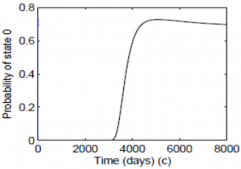
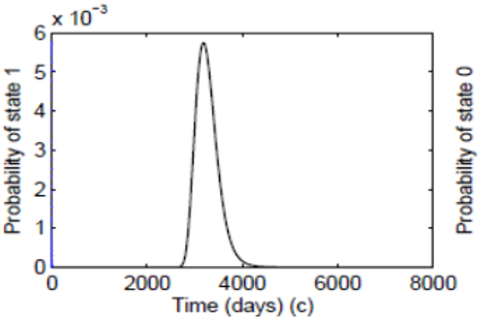
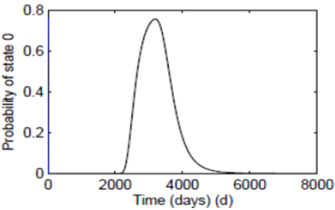
Figure 5. Degrading and failure state probabilities

6a.png

6b.png

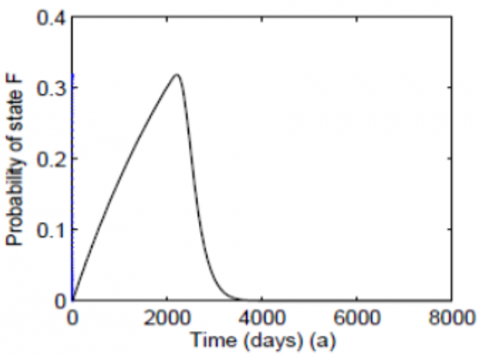
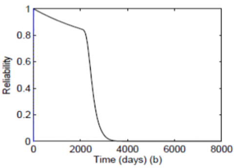
Figure 6. Catastrophic failure state (a) and Reliability changing (b)

From Figure 5(d), the probability of reaching a severe failure state (distinct from catastrophic failure) caused by continuous degradation peaks at 0.75 at 9.5 years. This indicates that the combined effects of both degradation processes (general wear and oil aging) become overwhelmingly dominant, rendering the OCB largely non-functional or unreliable by this time. Maintenance actions are thus critical well before this point. As shown in Figure 6(a), the probability of catastrophic failure now reaches 0.16 (16%) at only 7 years of operation a notable acceleration compared to the single-degradation scenario (0.2 at 9 years). This means the system becomes critically vulnerable to total breakdown much earlier, necessitating more aggressive preventive maintenance.

The reliability plot (Figure 6(b)) demonstrates that system failure is probable after just 10 years without intervention 4 years less than the single-degradation case. This quantifies the detrimental impact of including oil aging as a second degradation process. The reliability function remains influenced by random shocks, but the compounding effect of dual degradation mechanisms is now the primary driver of failure. Comparing to the initial state (Figure 5(a)), the system again transitions from a high-probability healthy state to degraded and failed states much more rapidly, reinforcing the dominant role of cumulative degradation.