Ganesh Karthik Muppagowni![]() | Srihari Varma Mantena
| Srihari Varma Mantena![]() | Phanikanth Chintamaneni
| Phanikanth Chintamaneni![]() | Srinivasulu Chennupalli
| Srinivasulu Chennupalli![]() | Sudhakar Yadav Naladesi
| Sudhakar Yadav Naladesi![]() | Ramesh Vatambeti*
| Ramesh Vatambeti*![]()
© 2023 IIETA. This article is published by IIETA and is licensed under the CC BY 4.0 license (http://creativecommons.org/licenses/by/4.0/).
OPEN ACCESS
Automated video surveillance systems (AVSs) have recently become vital for ensuring public safety, particularly at events with huge audiences like sporting events. Machine (ML) and deep learning (DL) open the way for computers to think like humans even further by including training and learning components, which artificial intelligence (AI) already provides. In order to evaluate and make sense of surveillance data acquired by fixed or mobile cameras mounted indoors or outdoors, DL algorithms require data labelling and high-performance processors. Recent advances in generative adversarial networks (GANs) for image synthesis and creation in VSSs have made it a hot topic in the field of study to establish if a given input is typical or atypical. Therefore, this research presents a better GAN network to recognise human gaits and to distinguish between human actions that are normal and pathological in VSSs. To achieve this goal, we first combine global and local features to enhance learning in crucial local regions that include multiple key points. Two, we use metric learning to pull out shared and unique characteristics. After features have been retrieved, they are used as input by the classification module in order to identify GAN-generated pictures. DMO is used in this study to perform hyper-parameter optimization (HPO) in GAN, which provides significant metaheuristic balance between the survey and misuse phases. The suggested model outperformed the existing model on all three datasets (CASIA-A, B, and C) used in the validation process. The proposed model had an accuracy of 98.48% on the A dataset and 99.87% on the B dataset, whereas the previous model had an accuracy of almost 94% on both datasets.
video surveillance system, generative adversarial networks, human gait recognition, dwarf mongoose optimization, hyper-parameter optimization
The computer vision community has become more interested in human gait detection from video in recent years, despite the task's reputation for being difficult and fraught with problems. Gait recognition is seen as a possible next-generation method [1], whereas other biometric technologies like facial recognition and fingerprinting are seen as current-generation techniques. Gait recognition has numerous advantages over other biometrics, including the fact that it does not require the subject's active participation or physical touch, and that the target data does not need to be extremely high-resolution or extremely close up to be effective. It is also hard to hide one's stride. Criminals often hide their identities by using disguises that render facial recognition systems useless. Gait recognition is the only practical and efficient means of identification in such cases [2]. As a result, gait recognition is extremely sensitive to both the functional structure of the human body and the dynamics of human walking motion. In the past decade, HGR has emerged as a vision. Gait recognition has various uses in industry, including biometrics [3, 4], which is why it is widely used in fields like surveillance and healthcare. Several aspects affect gait recognition despite the unique qualities of gait features themselves; they include camera viewpoints, circumstances, clothing variations, and beneath the feet [5]. Thus, it is essential for correct gait categorization [6] to develop a strong enough framework to overcome these challenges. Furthermore, some biological markers, such as electromyography (EMG) [7-9], inertial sensors [10, 11], and plantar pressure [12], are also relevant for gait analysis. Such techniques allow for the analysis of human gait, for instance, by tracking muscle activity as a person walks. In recent years, gait recognition procedures have advanced to the point that they may be employed in a variety of "real-world" settings, including video surveillance, crime deterrence, and forensic identification [13, 14].
Gait recognition and emotional state [15]. There is still a long way to go before gait recognition can be considered solved. Creating an effective approach to gait identification that is invariant to multiple alterations, such as viewing-angle changes and the wearing or carrying circumstances of the individuals, is difficult. Because of this, we view the challenge of gait recognition in the presence of such variables or changes as our primary research emphasis. These confounding factors are common in the real world and can have a major effect on gait recognition accuracy. Feature extraction is a crucial part of gait recognition [16], which is the process of extracting signals that may be used for recognition from video arrangements that depict a person walking. This is crucial since there are several potential methods for signal extraction from a gait video series. Therefore, it is essential that as much discriminating information as possible be condensed throughout the feature extraction process. Therefore, deep learning-based methods might be the answer to this challenging recognition issue.
Several layers of a convolution neural network (CNN) are used to extract the underlying structure and semantics of a picture, making it a form of deep learning. CNN employs some of its layers for down sampling and others for network activation [17]. Some superfluous or useless characteristics are also removed from the raw pictures when the deep features are retrieved. Improved classification accuracy requires further development of such characteristics. Deep learning hyper-parameter optimization has been developed by researchers to improve the precision of DL methods.
Problem Statement: The primary issues that are tackled in this study are:
Contributions: To address these problems, a novel framework is developed that employs deep learning and an assortment of optimal parameters for the classifier to improve human gait identification. Here are some of the major contributions:
Here's how the rest of the manuscript is laid out: In Section 2, we will go through some of the most recent developments in gait recognition technology. In Section 3, we describe the dataset and its methods. The suggested method's findings are presented in Section 4, and an immediate and last thought are offered in Section 5.
Using video sequences, Khan et al. [18] presented a completely IACO method for HGR. There are primarily four stages to the suggested structure. The initial process included standardising the database within the context of a moving image. Second, the characteristics of the dataset are used to inform the selection and refinement of one of two pre-trained replicas, ResNet101 and InceptionV3. The two adapted models were then trained by transfer learning, and features were retrieved. The retrieved characteristics were optimised with the help of the IACO algorithm. The best characteristics were chosen using IACO and then fed into a Cubic Support Vector Machine for classification. Multiclass analysis is used by the cubic support vector machine. The accuracy was 95.2%, 93.92%, and 98.2% across the board, respectively, when tested on the CASIAB dataset from 0, 18, and 180 degrees. The suggested method has also been compared to other approaches and found to be superior in terms of accuracy and computing time.
The solution described by Sharif et al. [19] efficiently deals with real-time issues such as changing viewing angles and different gaits. The proposed novel framework consists of the following steps: (a) capturing video in real-time; (b) extracting features. The most cutting-edge machine learning classifiers are then used to categorise the characteristics with the greatest degree of discriminatory power. Both the CASIA B dataset and a real-time recorded dataset were used to fuel the simulation process. Specifically, the accuracy is between 95.26 and 96.60 percent on several datasets. The findings demonstrate the superiority of our suggested framework over numerous established methods.
The Vision Transformer (ViT) is used for gait detection in Gait-ViT by Mogan et al. [20], which incorporates an attention mechanism. When implementing the suggested Gait-ViT, we first averaged a series of photos taken during the gait cycle to produce the gait energy image. Next, flattening and patch embedding are used to convert the picture patches into sequences. In order to recover the patch positions, position embedding is performed on the sequence of patches alongside patch embedding. After receiving the vector sequence, the Transformer encoder was used to generate the final gait representation. When determining a sequence's categorization, the initial item was fed into a multi-layer perceptron for label prediction. The Vision Transformer model's superior performance over state-of-the-art approaches is demonstrated by the suggested method's results.
In order to recognise gaits captured by the Kinect, Bari and Gavrilova [21] suggest using a convolutional neural network called KinectGaitNet. Each joint's 3D coordinates are modified during the gait cycle to yield a new input illustration. As an alternative to employing hand-crafted features, the suggested KinectGaitNet was trained directly on the 3D input representation. The KinectGaitNet architecture eliminates the need for resampling gait cycles, and the residual learning approach guarantees precision without deterioration. With an accuracy of 96.91 percent on the UPCV and 99.33 percent on the KGB dataset, the proposed deep learning architecture outperforms all existing algorithms for Kinect-based gait identification. To the best of our knowledge, this technique was the first deep learning-based architecture to use a novel 3D input representation of joints. With fewer parameters and less time spent in inference, it outperforms both conventional and deep learning techniques.
The performance under different variables was improved by combining a pre-trained VGG-16 model with a multilayer perceptron, as described by Mogan et al. [22]. First, we averaged the silhouettes throughout a walking cycle to get the gait energy picture. In order to understand the gait characteristics of the obtained gait energy picture, we first apply transfer learning and fine-tuning approaches to the pre-trained VGG-16 model. After that, we used a multilayer perceptron to figure out how each gait trait was connected to its respective person. At last, the classification layer determines the topic. The CASIA-B dataset, OU-ISIR dataset D, and OU-ISIR big population dataset are used in experiments to assess all of the datasets examined.
In this paper, Khan et al. [23] offer a lightweight DL approach to human gait identification. The suggested procedure involves a series of stages for selecting features for classification using pretrained deep models. As a starting point, we evaluate two lightweight pretrained models and make adjustments to them by adding or freezing layers in the centre of the network. Subsequently, analysis was used to accomplish the fusion, and subsequently, an enhanced moth-flame optimization approach was used to get optimal results. Extreme learning machines are used to classify the final optimal features (ELM). Experiments were run on CASIA B and TUM GAID, two publicly available datasets, with an average accuracy of 91.20 and 98.60%, respectively. The proposed method was found to be more precise than current state-of-the-art procedures.
Lower limbs EMG-based gait identification algorithms are made more reliable and accurate by Cai et al. [24]. The work began by presenting a feature combination selection–based Linear Discriminant Analysis–Particle Swarm Optimization–Long Short-Term Memory (LDA–PSO–LSTM) method, which was then experimentally evaluated for its identification accuracy. With a maximum accuracy of 97.02%, LDA-PSO-LSTM achieved an average recognition rate of 94.89%. Second, we examined the LDA-recognition LSTM's accuracy (92.17%) and compared it to other methods. In experiments, the PSO optimization model demonstrated strong recognition capabilities. At the end, we compared LDA-LSTM to every possible combination of classifiers and found that LDA-LSTM yielded the greatest recognition rate. The outcomes show that LDA-PSO-LSTM has clear benefits as a classification model for gait recognition.
3.1 Dataset
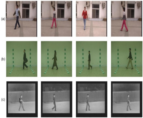
In this study, we used the CASIA A gait dataset, the CASIA B gait dataset, and the CASIA C gait dataset [25], all of which are accessible for public use. Figure 1 displays the sample frames for each dataset. Here is a quick summary of several connected data sets:
Figure 1. Frames representative of the gait recognition datasets that were chosen
CASIA Field recordings from two consecutive days were used to create a gait dataset. Twenty participants walked through three different camera angles—lateral (0°), oblique (45°), and frontal (90°)—to create this dataset. With an average gait sequence duration of around 90 frames collected at 25 fps and a resolution of 352x240, the dataset has a total of 240 gait sequences. A total of 168 video sequences were used in this study, some for training and some for assessment.
The CASIA B gait dataset is frequently employed as a database for multi-view gait identification. A total of 124 participants (93 men and 31 women) were videotaped while walking around an indoor arena from 11 various angles utilising USB cameras. Each of the 18 possible directions of view is ordered as follows: 0 degrees, 18 degrees, 36 degrees, 54 degrees, 72 degrees, 90 degrees, 108 degrees, 126 degrees, 144 degrees, 162 degrees, and 180 degrees Six video sequences of the same person wearing a coat (WC) and two video sequences of the same person carrying a bag (CB) were captured to serve as gait sequences for multi-view. The frame size of the movies was 320 x 240, and the recording speed was 25 frames per second. That means there are a total of 13,640 video sequences in the dataset, or 1011124. Only videos with a 90-degree field of view were evaluated for this post, for a grand total of 1240 clips. The 70:30 validation method was used, as in the CASIA A dataset.
The CASIA C gait dataset is a thermal camera night time gait data set. For the dataset, 153 participants recorded gait sequences in a natural setting (130 males and 23 females). Walk with a bag (CB), slow walk (SW), normal walk (NW), and fast walk (QW) are the four types of gait changes that were recorded in each gait sequence (QW). During the recording process, participants walked a total of eight times: four times at a normal pace, twice while carrying a bag, twice at a slower pace, and twice at a faster pace. As a result, 1530 gait sequences were captured at a rate of 320 per 240. In addition, the suggested system was trained and tested with 1071 video sequences.
3.2 Real-time processing
Since the well-known application of intelligent video surveillance monitors security in real time, utilising numerous cameras in defence systems, the study of HGR in real time using video processing is a thriving field of study. However, a superior system is not yet accessible because of the significant difficulties in this field, such as video analysis or comprehension. Football and cricket, in particular, use real-time video processing to take swift action in the face of violence. Although more recent real-time gait identification systems have been established, there are still significant restrictions to achieving the necessary performance [25, 26].
3.3 Low-quality video processing
High-Gain Regression (HGR) in low-quality video arrangements is challenging because of the crowded backdrop and concealed information. Since the information in video is compressed, potentially leading to the loss of critical characteristics, image solidity is an essential part of video processing. As a result, effective improvement techniques are required to provide higher-quality video frames and a consequently higher recognition rate.
3.4 Proposed GAN
Most face detection algorithms that use GAN only look at global features. But the local characteristics have been very important in the field of gait recognition. So, to improve the ability to generalise, we recommend putting more emphasis on learning about important local areas and combining global and local features. In this section, the proposed algorithm's main structure is explained first, and then each of its three modules—the global feature extraction module and the classification module—is explained in detail.
3.4.1 Main architecture
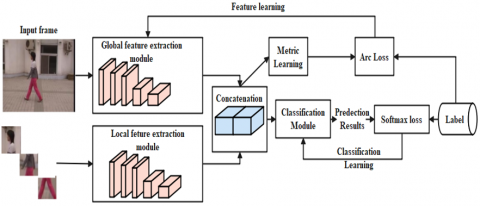
Figure 2. Main architecture of the projected algorithm
As shown in Figure 2, the overall construction of the projected algorithm comprises two steps: feature learning and classification learning. Notice that the cubes in Figure 2 are just some simple signs rather than detailed structures. The detailed structures of three modules are given in the following three subsections. In the feature learning step, firstly, the features from the global and local feature extraction modules are merged; secondly, metric learning is used to further learn common features in the same type of gait and discriminative features between natural and GANs-generated images. Metric learning transforms the merged features into an embedding feature with fixed dimensions (128 dimensions in this paper) via a fully connected (FC) layer. Thereafter, the training loss is applied to supervise the metric learning. By minimising the training loss defined in Eq. (1), gait images with the same label will have similar features after being extracted by the feature extraction modules. In the classification learning step, the features extracted from the global and local modules are fed into the classification module to obtain the predicted results. Notice that the metric learning is not considered in the testing phase because it needs labels to supervise the feature distribution and there is no label when making decisions. The input images are processed by the feature extraction module and the classification module to directly predict the result. The details of three modules are presented in the following three subsections.
Given the feature X and weight vector W, the training loss is presented as follow,
$L_{\text {gait loss predict }} \,\,=-\frac{1}{N} \sum_{i=1}^N \log \frac{e^{s\left(\cos \left(\theta_{y_i}+m\right)\right)}}{e^{s\left(\cos \left(\theta_{y_i}+m\right)\right)} \quad \,\,\, +\sum_{j=1, j \neq y_i}^n \quad e^{s \cos \theta_j}}$ (1)
where, N and n signify the batch size and the sum of categories, correspondingly, θ denotes the angle between W and X, s represents the scaling factor, m represents the additive angular margin penalty, and yi is the label value of the i-th sample.
3.4.2 Global feature extraction module
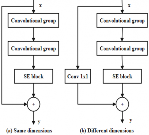
SE-Residual block is a main component in the global feature extraction module. It embeds the SE block is presented in Figure 3. As exposed in Figure 3, if the input x and the output y have matched dimensions, we use the structure of Figure 3(a), otherwise Figure 3(b) (matching dimensions by 1×1 convolution). Each architecture of SE-Residual block has two convolutional groups and a SE block. A convolutional group includes convolution (Conv), batch normalization (BN), and ReLU activation. In real application, the dimensions of the input and output of each SE-Residual block are already known when we design a network model, thus choosing Figure 3(a) or Figure 3(b) is also known in the model design phase.
Figure 3. The input and output dimensions might be the same or different, depending on the architecture of the SE-Residual blocks
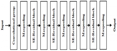
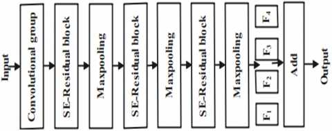
The detailed architecture of the global feature extraction module is shown in Figure 4. This module is composed of four SE-Residual blocks, a convolutional group, and four maxpooling layers. The SE-Residual block can extract inherent effectiveness of features. The global feature extraction module is a relatively shallow network due to the small size of input face and the uncomplicated classification task. Regarding the network parameters, the kernel size of the convolutional group is 7×7 with stride 1, while those of the rest of convolutional layers in four SE-Residual blocks are 3×3 with stride 1; The number of kernels in the convolutional group and four SE-Residual blocks is 32, 32, 64, 64, and 128, respectively; The kernel sizes of all maxpooling layers are 2×2 with stride 2.
Figure 4. Construction of the global feature extraction component
3.4.3 Local feature extraction module
The key-points are some important landmarks in the HGR images. So, they are utilized to determine the important local areas. We use the gait landmark detection code from Dlib C++ library to collect 68 keypoints. Then, we find that these key-points mainly distribute in four areas, i.e., ankle points, toe points, shoulder points and hand points. To obtain these four areas, a rectangular is used to crop each area in each gait image. The rectangular is the smallest rectangle containing all key-points near each area. Besides, to contain each area completely, each rectangular is extended around 10 pixels. Hereafter, four cropped patches are normalized to 32×32.
Figure 5. Architecture of the local feature extraction component
The detailed architecture of the local feature extraction module is shown in Figure 5. Compared with the global module as shown in the Figure 4, a group of SE-Residual blocks and a maxpooling layer are removed because of the following concatenation operation between the local module and the global module, whose outputs should have the same resolution. The four cropped areas obtained from the extracted key-points are fed into the residual attention network one by one to output four groups of features, i.e., F1, F2, F3, and F4. Then, these four groups of features are fused by an add operation to obtain the final feature of the local module. The number of kernels in the first convolutional group and three SE-Residual blocks is 32, 32, 64, and 128, respectively.
3.5 Classification module
A layer make up this component. For the convolutional layer, a kernel size of 3x3 and a stride of 1 is used. Two neurons constitute the FC layer (two categories: natural and generated).
Softmax loss, the most common classification loss function, is taken into account for its ability to efficiently oversee the classification module,
$L_{\text {softmax }}=-\frac{1}{N} \sum_{i=1}^N \log \frac{e^{W_{y i}^T x_i+b_i}}{\sum_{j=1}^n e^{W_j^T x_i+b_j}}$ (2)
where, N is the sum of samples in a batch, n is the sum of categories, x i is a sample from deep feature x, y i is a sample's label, W is a weight vector, and b is a bias factor. Loss L softmax should be kept as small as possible. DMO, defined in Section 3.5.1, is the ideal choice for the weight and bias terms specified by HPO.
3.5.1 Dwarf mongoose optimization algorithm
Unlike foraging, which is done in groups of dwarf mongooses, food seeking is a solitary activity. These creatures are seminomadic, so when they construct a sleeping sound, they do it near an especially rich food source. To find optimal solutions, the system simulates the behaviour of this creature statistically.
Initialization is a random process in all population-based optimization techniques. After then, all solutions converge on the global best optimum as a result of the intensification and diversification criteria. In a similar vein, the DMO begins its solution by seeding the network with a random set of candidates. This sample population is produced at random between the minimum and maximum allowable values for a given issue.
$X=\left[\begin{array}{cccccc}x_{1,1} & x_{1,2} & \ldots & \ldots & x_{1, d-1} & x_{1, d} \\ x_{2,1} & x_{2,2} & \ldots & \ldots & x_{2, d-1} & x_{2, d} \\ \vdots & \vdots & \vdots & \cdot^{\cdot^{\cdot}} & \vdots & \vdots \\ x_{n, 1} & x_{n, 2} & \ldots & \ldots & x_{n, d-1} & x_{n, d}\end{array}\right]$ (3)
where, X represents the current candidate population that has been produced at random using Eq. (4), x (i,j) represents the location of the ith population along the jth dimension, n represents the total size of the population, and d denotes the problem's dimension.
xi, j=unifrnd(VarMin, VarMax, VarSize) (4)
where, unifrnd is a uniformly distributed random integer, VarMin is the minimum bound, VarMax the maximum bound, and VarSize the size of the problem space. After each iteration, the best solution is the best one found so far.
Exploitation (each mongoose conducts a comprehensive search in each search region), also known as bountiful food source or new resting mound), also known as diversification, are the two phases of the DMO. The DMO's alpha group, scout group, and babysitters are the three main social institutions responsible for implementing the aforementioned stages.
The apex female () is the primary decision maker in the household and is chosen using the Eq. (5).
$a=\frac{f i t_i}{\sum_{i=1}^n f i t_i}$ (5)
The sum of n and bs is equal to the number of mongooses that are in the alpha group. The symbol for the number of babysitters is "bs," and the sound made by the female alpha to direct the attention of the other members of the unit is represented by the letter "peep."
The presence of ample food is what determines the sleeping mound, as seen in the Eq. (6).
$X_{i+1}=X_i+p h i * peep$ (6)
At the end of each cycle, the sleeping sound is evaluated using Eq. (7), where phi is a random value in the range [1, 1].
$s m_i=\frac{fit_{i+1}-f i t_i}{\max \left\{\left|f i t_{i+1}, f i t_i\right|\right\}}$ (7)
Once a sleeping sound is discovered, the mean is calculated using Eq. (8)
$\varphi=\frac{\sum_{i=1}^n s m_i}{n}$ (8)
Once the criteria for switching babysitters have been met, the scouting phase begins, during which the next sleeping sound is evaluated based on an alternate food source.
Since mongoose are not known to return to their previous sleeping sound, the scouting party must always be on the lookout for new ones. In DMO, the mongoose is known to forage and scout at the same time, presumably because the further the unit forages, the greater its chances of discovering the next sleeping sound. With the help of Eq. (9).
$X_{i+1}=\left\{\begin{array}{ccc}X_i-C F * \text { phi } * \text { rand } *\left[X_i-\vec{m}\right] & \text { if } & \varphi_{i+1}>\varphi_i \\ X_i+C F * \text { phi } * \operatorname{rand} *\left[X_i-\vec{m}\right] & \text { else }\end{array}\right.$ (9)
where, rand is a random number among $[0,1], C F=\left(1-\frac{\text { iter }}{\text { Max }_{\text {iter }}}\right)^{\left(2-\frac{\text { iter }}{\operatorname{Max}_{i t e r}}\right)}$ shows the parameter that guides iterations. $\vec{M}=\sum_{i=1}^n \frac{x_i \times s m_i}{x_i}$ indicates the direction of force that drives a mongoose to a new den.
In this part, we show how our proposed system has been tested with many data sets and evaluated with various metrics. In order to do this, we used a 70:30 split for training and testing on three publicly available datasets. After data partitioning, a pre-trained model was loaded, and activation was determined using cross entropy. The DMO algorithm decided on a learning rate of 0.001 and an initial mini batch size of 64. This procedure was built in Matconvnet, a deep learning toolkit in MATLAB2018a. The sensitivity, precision rate, false-negative rate, false-positive rate, area under the curve (AUC), F1-score, and accuracy were used to evaluate the system. The total amount of time needed by the suggested system to do a categorization was also determined.
4.1 Performance metrics
The confusion matrix for the binary classification was created to assess the efficacy of the suggested technique for labelling human anomalies. Comparisons were made between the GAN-DMO model's results and those of similar pre-existing models based on HGR. The effectiveness of the proposed method was evaluated using four statistical indices (True Positive [TP], False Positive [FP], False Negative [FN], and True Negative [TN]) computed from the resultant confusion matrix (TN). Statisticians used these numbers to determine things like accuracy, sensitivity, specificity, and the F1-Score.
Accuracy $=\frac{T P+T N}{T P+F P+T N+F N}$ (10)
Sensitivity $=\frac{T P}{T P+F N}$ (11)
Specificity $=\frac{T N}{T N+F P}$ (12)
Precision $=\frac{T P}{F P+T P}$ (13)
$F 1-$ Score $=2 * \frac{\text { Precision } * \text { Sensitivity }}{\text { Precision }+ \text { Sensitivity }}$ (14)
Area Under Curve (AUC) and Receiver Operating Characteristics (ROC) curves were created to quantitatively estimate the performance of the proposed GAN-DMO model. Tables 1 and 2 compare the proposed GAN model with and without optimization (DMO) on three separate datasets.
Table 1. Comparison of the average performance metrics of GAN without DMO
|
Metric |
CASIA B |
CASIA C |
CASIA A |
|
Precision |
95.73% |
66.74% |
95.42% |
|
F1-score |
96.73% |
79.73% |
95.41% |
|
Accuracy |
96.74% |
90.66% |
95.42% |
|
Sensitivity |
94.73% |
92.00% |
95.40% |
|
Specificity |
94.95% |
88.74% |
98.85% |
|
AUC |
97.71% |
93.67% |
96.35% |
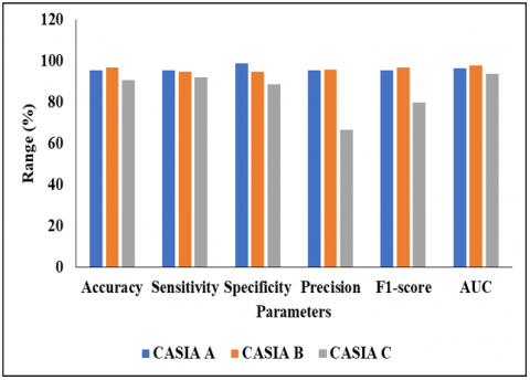
Figure 6. Graphical comparison of Proposed GAN model without DMO
In the analysis of accuracy, the GAN model achieved 95.40% on A dataset, 96.73% on B dataset and 90.65% on C dataset. When the GAN model is tested with three datasets such as A, B and C, it achieved 95.40%, 94.73% and 92% of sensitivity. In the A dataset, the GAN model achieved 98.85% of specificity, 95% of precision and F1-score and 96.35% of AUC, where the GAN model achieved nearly 94% to 97% of specificity, precision, F1-score and AUC on CASIA B dataset. While comparing with all datasets, CASIA C provides low performance on GAN model, i.e., it achieved 88.74% of specificity, 66.74% of precision, 79.73% of F1-score and 93.67% of AUC. Figure 6 presents the graphical comparison of proposed GAN without DMO for three datasets.
Table 2. Analysis of GAN model with DMO
|
Metric |
CASIA B |
CASIA C |
CASIA A |
|
Precision |
99.848 |
75.00 |
98.557 |
|
F1-score |
99.872 |
85.525 |
98.457 |
|
Accuracy |
99.78 |
93.75 |
98.482 |
|
Sensitivity |
99.864 |
99.632 |
98.523 |
|
Specificity |
99.969 |
92.426 |
99.579 |
|
AUC |
99.85 |
95.05 |
99.78 |
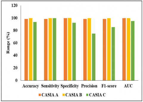
When the GAN model is tested with DMO, it achieved better performance on three different datasets such as A, B and C. In the CASIA A dataset, the GAN-DMO model achieved nearly 98% to 99% of accuracy, sensitivity, specificity, precision, F1-score and AUC. In the analysis of CASIA C dataset, the proposed GAN-DMO model achieved 93% of accuracy, 99% of sensitivity, 92% of specificity, 75% of precision, 85.52% of F1-score and 95% of AUC. In the CASIA B dataset, the proposed model achieved 99% on all metrics such as accuracy, precision, sensitivity, specificity, F1-score and AUC. Figure 7 presents the graphical analysis of proposed GAN-DMO for all dataset.
Figure 7. Analysis of GAN-DMO model for three datasets
4.2 Comparative analysis of proposed model
Table 3 presents the techniques in terms of all datasets. The existing techniques such as IACO [18] on CASIA B, ResNet [19] on CASIA B, ViT [20] on CASIA-B, VGG-16 [22] on CASIA-B, ELM [23] on CASIA-B are considered, but the proposed GAN-DMO model uses three datasets. Therefore, the techniques from [18-23] are implemented with these datasets and results are averaged.
Table 3. Comparative analysis of GAN-DMO with various techniques
|
Techniques |
CASIA A |
CASIA B |
CASIA C |
|
IACO |
0.8863 |
0.8775 |
0.8207 |
|
ResNet |
0.8997 |
0.8925 |
0.8297 |
|
ViT |
0.9111 |
0.9098 |
0.8775 |
|
VGG-16 |
0.9088 |
0.9095 |
0.8525 |
|
ELM |
0.9437 |
0.9449 |
0.8965 |
|
GAN-DMO |
0.9848 |
0.9987 |
0.9377 |
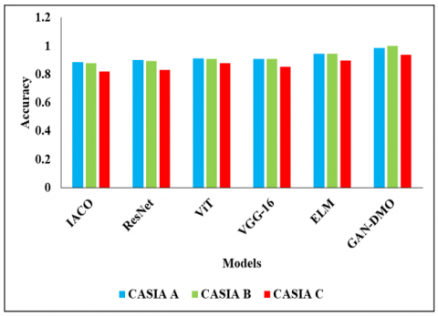
In the CASIA-A dataset, the existing techniques such as IACO, ResNet achieved 88% to 89%, VGG and ViT achieved 90% to 91%, ELM achieved 94% and proposed model achieved 98.48%. The reason for better performance is that the GAN’s HPO is optimized by DMO, where existing techniques didn’t focus on tuning the parameters for high classification accuracy. Likewise, the analysis of CASIA B dataset, the existing techniques achieved nearly 87% to 94% and 82% to 89% of accuracy on CASIA C, where proposed model achieved 99% and 93% of accuracy on CASIA-C dataset. Figure 8 provides the graphical representation of proposed model with existing techniques.
Figure 8. Analysis of accuracy on three datasets
Our suggested general method combines global and local characteristics with metric learning based on the training loss of gait prediction to enhance the generalisation potential of existing GAN-generated gait image recognition systems. The experimental findings show that the suggested approach outperforms several pre-existing algorithms and provides an acceptable generalisation capacity, with average accuracy values exceeding 0.99 across all three testing datasets. Here are some of the more important ones: By combining global and local features extracted by the residual attention network, a) the learning on crucial local areas is reinforced, and b) the metric learning is applied to obtain common features in the same type of gait images and discriminative features between natural and GAN-generated gait in the feature learning phase. There is little doubt that the suggested method greatly benefits from HPO optimization since its performance is greatly enhanced. Possible future actions are listed here.
[1] Ravikiran, R., Kumar, G.S., Pareek, P.K. (2023). Analyzing Human Speech Using Gait Recognition Technology by MFCC Technique. In: Khanna, A., Gupta, D., Kansal, V., Fortino, G., Hassanien, A.E. (eds) Proceedings of Third Doctoral Symposium on Computational Intelligence. Lecture Notes in Networks and Systems, vol 479. Springer, Singapore. https://doi.org/10.1007/978-981-19-3148-2_61
[2] Saleem, F., Khan, M.A., Alhaisoni, M., Tariq, U., Armghan, A., Alenezi, F., Choi, J.I., Kadry, S. (2021). Human gait recognition: A single stream optimal deep learning features fusion. Sensors, 21(22): 7584. https://doi.org/10.3390/s21227584
[3] Kececi, A., Yildirak, A., Ozyazici, K., Ayluctarhan, G., Agbulut, O., Zincir, I. (2020). Implementation of machine learning algorithms for gait recognition. Engineering Science and Technology, an International Journal, 23(4): 931-937. https://doi.org/10.1016/j.jestch.2020.01.005
[4] Gupta, A., Semwal, V.B. (2020). Multiple task human gait analysis and identification: Ensemble learning approach. In: Mohanty, S.N. (eds) Emotion and Information Processing. Springer, Cham. https://doi.org/10.1007/978-3-030-48849-9_12
[5] Khan, M.A., Kadry, S., Parwekar, P., Damaševičius, R., Mehmood, A., Khan, J.A., Naqvi, S.R. (2021). Human gait analysis for osteoarthritis prediction: A framework of deep learning and kernel extreme learning machine. Complex & Intelligent Systems, 1-19. https://doi.org/10.1007/s40747-020-00244-2
[6] Liu, C., Yan, W.Q. (2020). Gait recognition using deep learning. In Handbook of Research on Multimedia Cyber Security, pp. 214-226. IGI Global. https://doi.org/10.4018/978-1-7998-2701-6.ch011
[7] Wang, X., Yan, W.Q. (2020). Human gait recognition based on frame-by-frame gait energy images and convolutional long short-term memory. International Journal of Neural Systems, 30(1): 1950027. https://doi.org/10.1142/S0129065719500278
[8] Jiang, X., Zhang, Y., Yang, Q., Deng, B., Wang, H. (2020). Millimeter-wave array radar-based human gait recognition using multi-channel three-dimensional convolutional neural network. Sensors, 20(19): 5466. https://doi.org/10.3390/s20195466
[9] Zou, Q., Wang, Y., Wang, Q., Zhao, Y., Li, Q. (2020). Deep learning-based gait recognition using smartphones in the wild. IEEE Transactions on Information Forensics and Security, 15: 3197-3212. https://doi.org/10.1109/TIFS.2020.2985628
[10] Terrier, P. (2020). Gait recognition via deep learning of the center-of-pressure trajectory. Applied Sciences, 10(3): 774. https://doi.org/10.3390/app10030774
[11] Wang, X., Zhang, J., Yan, W.Q. (2020). Gait recognition using multichannel convolution neural networks. Neural Computing and Applications, 32(18): 14275-14285. https://doi.org/10.1007/s00521-019-04524-y
[12] Hnatiuc, M., Geman, O., Avram, A.G., Gupta, D., Shankar, K. (2021). Human signature identification using IoT technology and gait recognition. Electronics, 10(7): 852. https://doi.org/10.3390/electronics10070852
[13] Gul, S., Malik, M.I., Khan, G.M., Shafait, F. (2021). Multi-view gait recognition system using spatio-temporal features and deep learning. Expert Systems with Applications, 179: 115057. https://doi.org/10.1016/j.eswa.2021.115057
[14] Mehmood, A., Khan, M.A., Sharif, M., Khan, S.A., Shaheen, M., Saba, T., Riaz, N.. Ashraf, I. (2020). Prosperous human gait recognition: An end-to-end system based on pre-trained CNN features selection. Multimedia Tools and Applications, 1-21. https://doi.org/10.1007/s11042-020-08928-0
[15] Anusha, R., Jaidhar, C.D. (2020). Clothing invariant human gait recognition using modified local optimal oriented pattern binary descriptor. Multimedia Tools and Applications, 79: 2873-2896. https://doi.org/10.1007/s11042-019-08400-8
[16] Khera, P., Kumar, N. (2020). Role of machine learning in gait analysis: A review. Journal of Medical Engineering & Technology, 44(8): 441-467. https://doi.org/10.1080/03091902.2020.1822940
[17] Zhang, Z., He, T., Zhu, M., Sun, Z., Shi, Q., Zhu, J., Dong, B., Yuce, M.R., Lee, C. (2020). Deep learning-enabled triboelectric smart socks for IoT-based gait analysis and VR applications. npj Flexible Electronics, 4(1): 29. https://doi.org/10.1038/s41528-020-00092-7
[18] Khan, A., Javed, M., Alhaisoni, M., Tariq, U., Kadry, S., Choi, J., Nam, Y. (2022). Human gait recognition using deep learning and improved ant colony optimization. CMC-Computers Materials & Continua, 70(2): 2113-2130. http://dx.doi.org/10.32604/cmc.2022.018270
[19] Sharif, M.I., Khan, M.A., Alqahtani, A., Nazir, M., Alsubai, S., Binbusayyis, A., Damaševičius, R. (2022). Deep learning and kurtosis-controlled, entropy-based framework for human gait recognition using video sequences. Electronics, 11(3): 334. https://doi.org/10.3390/electronics11030334
[20] Mogan, J.N., Lee, C.P., Lim, K.M., Muthu, K.S. (2022). Gait-ViT: Gait Recognition with Vision Transformer. Sensors, 22(19): 7362. https://doi.org/10.3390/s22197362
[21] Bari, A.H., Gavrilova, M.L. (2022). KinectGaitNet: Kinect-based gait recognition using deep convolutional neural network. Sensors, 22(7): 2631. https://doi.org/10.3390/s22072631
[22] Mogan, J.N., Lee, C.P., Lim, K.M., Muthu, K.S. (2022). VGG16-MLP: Gait Recognition with Fine-Tuned VGG-16 and Multilayer Perceptron. Applied Sciences, 12(15): 7639. https://doi.org/10.3390/app12157639
[23] Khan, M.A., Arshad, H., Damaševičius, R., Alqahtani, A., Alsubai, S., Binbusayyis, A., Nam, Y. and Kang, B.G. (2022). Human gait analysis: A sequential framework of lightweight deep learning and improved moth-flame optimization algorithm. Computational intelligence and neuroscience, 2022: 8238375. https://doi.org/10.1155/2022/8238375
[24] Cai, S., Chen, D., Fan, B., Du, M., Bao, G., Li, G. (2023). Gait phases recognition based on lower limb sEMG signals using LDA-PSO-LSTM algorithm. Biomedical Signal Processing and Control, 80: 104272. https://doi.org/10.1016/j.bspc.2022.104272
[25] Arshad, H., Khan, M. A., Sharif, M.I., Yasmin, M., Tavares, J.M.R., Zhang, Y.D., Satapathy, S.C. (2022). A multilevel paradigm for deep convolutional neural network features selection with an application to human gait recognition. Expert Systems, 39(7): e12541. https://doi.org/10.1111/exsy.12541
[26] Agushaka, J.O., Ezugwu, A.E., Abualigah, L. (2022). Dwarf mongoose optimization algorithm. Computer Methods in Applied Mechanics and Engineering, 391: 114570. https://doi.org/10.1016/j.cma.2022.114570