Menaka Muthuramu![]() | Manimaran Rajendran*
| Manimaran Rajendran*![]()
© 2025 The authors. This article is published by IIETA and is licensed under the CC BY 4.0 license (http://creativecommons.org/licenses/by/4.0/).
OPEN ACCESS
This study investigates the thermal behavior of fins with temperature-dependent internal heat generation and thermal conductivity using the Taylor series method, a semi-analytical technique known for its simplicity and accuracy. Two key scenarios are analyzed: (1) internal heat generation as a function of fin temperature, and (2) both internal heat generation and thermal conductivity as temperature-dependent. Closed-form analytical expressions for temperature distribution and fin efficiency are derived for both cases. Results show that increasing the heat generation parameter significantly raises the temperature profile, with a peak temperature increase compared to the baseline case. When thermal conductivity decreases with temperature, heat accumulation becomes more pronounced, reducing fin efficiency. Parametric analysis further reveals that the Taylor series method not only matches the accuracy of established numerical methods such as the finite difference method (Scilab) but also offers computational simplicity and analytical insight. These findings underscore the method’s potential for efficiently solving complex nonlinear heat transfer problems in engineering applications.
mathematical modelling, convective fin temperature-dependent thermal conductivity, heat generation, Taylor series method, thermal analysis
The best tool for accelerating the rate of heat transfer is fins. They enhance the area of heat transmission and, as we know, the quantity of heat transport. Kraus et al. [1] provide a thorough examination of this subject. Fins are frequently used in factories, including electrical chips, freezing, car air conditioning, and chemical manufacturing equipment. Even though there are many other kinds of fins, the rectangular fin is the most common, most likely because of its straightforward form and simple production method. The thermal conductivity is considered to be constant for typical fin issues. Nonetheless, the impact of temperature on thermal conductivity must be regarded when there is a significant temperature difference between the fin's base and tip. Feeling the heat created in the fin as a function of temperature (from electric current, etc.) is also lifelike.
Using the least squares technique, Aziz and Bouaziz [2] forecasted the behavior of a longitudinal fin with internal heat production. They contrasted their findings using the dual series perturbation, variational iteration, and the homotopy perturbation (HPM) approaches. They discovered that this is more straightforward than other applicable approaches. The ideal fin design was determined by Razani and Ahmadi [3] by creating circular fins with random heat dispersion. Unal discussed the non-uniform heat production and heat transmission coefficients [4]. Convective fins with temperature-dependent thermal conductivity were developed [5]. Kundu [6] addressed a problem with thermal evaluation and design of uniformly thick horizontal fins.
The homotopy analysis method (HAM) was used [7, 8] to solve the nonlinear fin differential equation to assess the fin efficiency. Additionally, Ganji et al. [9] used HPM to study the temperature distribution for annual fins. Aziz and Khani [10] have examined the effects of temperature on a moving fin, considering the radiation losses. Bouaziz and Aziz [11] also introduced a twofold ideal linearization approach to provide a simple and accurate solution for the temperature distribution in a straight rectangular convective–radiative fin.
Recent research on heat transfer in fins with temperature-dependent properties has focused on improving analytical and semi-analytical methods to handle nonlinearities from variable thermal conductivity and internal heat generation. For example, Kumar et al. [12] used the Hermite collocation method to model semi-spherical fins, while Ananth Subray et al. [13] applied the Differential Transformation Method (DTM) to convective-radiative fins. Studies like Girish et al. [14] explored hybrid nanofluids in porous fins, revealing enhanced heat transfer and neural network-based models have shown promise for accurate temperature prediction Liu et al. [15]. These advances support more efficient thermal management designs in engineering applications. These are the latest developments in the study of temperature-dependent heat transfer fins.
Zhou [16] originally proposed the differential transformation method (DTM) idea in 1986 to handle both linear and nonlinear initial value issues in electric circuit analysis. The primary advantage of this approach is that it may be used directly for both linear and nonlinear differential equations without the need for linearization, discretization, or perturbation. Ghafoori et al. [17] solved the nonlinear oscillation problem using the DTMf. Hassan [18] used DTM for various differential equation systems and examined its convergence in several linear and nonlinear differential equation system cases. Abazari and Abazari [19] solved the generalized Hirota–Satsuma coupled KdV problem using the DTM and reduced differential transformation technique.
Rashidi et al. [20] used DTM to solve the mixed convection problem concerning an inclined flat plate buried in a porous medium; They used the Pade approximation to improve the solution's convergence. Abbasov et al. [21] observed approximations for the linear and nonlinear equations associated with engineering issues. The DTM was applied to a few PDEs and their linked counterparts in previous studies [22-25]. Kundu et al. [26] used the DTM. to forecast the performance of triangular and wet fins. Using analytical methods, Hatami and Ganji [27-30] and Hatami et al. [31] effectively resolved the heat transmission via porous fins of different forms.
The present paper has applied the Taylor series method to find the semi-analytical solution for fin temperature distribution and thermal conductivity. The model's semi-analytical solution may be obtained and compared to numerical data to demonstrate the method's high accuracy, simplicity, efficacy, and potential.
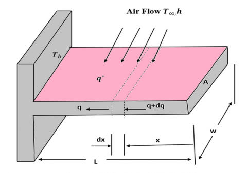
Heat transmission only occurs in the horizontal direction (x direction) because we assume the temperature change in the transfer direction is very small. Figure 1 depicts a schematic of the fin's geometry and other characteristics.
Figure 1. Diagrammatic representation of the fin shape and the source of heat production
The differential equation for the present problem may be expressed as [2].
$\frac{d^2 T}{d X^2}-\frac{h P}{k_0 A}\left(T-T_{\infty}\right)+\frac{q^*}{k_0}=0$ (1)
The boundary conditions are:
At $X=0, \frac{d T}{d X}=0$ (2)
At $X=L, T=T_b$ (3)
There are two primary scenarios when this issue is resolved. The governing equations for these two conditions are presented in the next subsections.
2.1 Case 1-Fin with temperature-dependent internal heat generation and constant thermal conductivity
In the first scenario, it is considered that the thermal conductivity is constant (k0) and the fin's heat production fluctuates with temperature as shown in Eq. (4).
$q^*=q_{\infty}^*\left(1+\varepsilon\left(T-T_{\infty}\right)\right)$ (4)
where, the internal heat production at temperature $T_{\infty}$ is represented by $q_{\infty}^*$ . The dimensionless variables listed below are provided.
$\begin{gathered}\theta=\frac{\left(T-T_{\infty}\right)}{\left(T_b-T_{\infty}\right)}, X=\frac{x}{L}, N^2=\frac{h P L^2}{k_0 A}, G=\frac{q_{\infty}^* A}{h P\left(T_b-T_{\infty}\right)} \\ \varepsilon_G=\varepsilon\left(T_b-T_{\infty}\right)\end{gathered}$ (5)
The Eq. (1) becomes in dimensionless form as follows:
$\frac{d^2 \theta(X)}{d X^2}-N^2 \theta(X)++N^2 G\left(1+\varepsilon_G \theta(X)\right)=0$ (6)
Boundary conditions are:
$X=0, \frac{d \theta(X)}{d X}=0$ (7)
$X=1 \theta(X)=1$ (8)
The exact solution of Eq. (6) becomes:
$\theta(X)=\frac{\left(1-G-G \varepsilon_G\right) \cosh \left(N \sqrt{1-G \varepsilon_G} X\right)}{\left(1-G \varepsilon_G\right) \cosh \left(N \sqrt{1-G \varepsilon_G}\right)}+\frac{G}{\left(1-G \varepsilon_G\right)}$ (9)
2.2 Previous results for Case 1
Previously, this problem was solved using various methods, which are summarised in Table 1 below.
Table 1. Analytical expression for the previous results for Case 1
|
S.No. |
Temperature |
Method |
Ref. |
|
1 |
$\theta(X)=\frac{\cosh (a X)}{\cosh (a)}$, where $a=\sqrt{N^2\left[1-G\left(1+\varepsilon_G\right)\right]}$ |
ASM |
[32] |
|
2 |
$\theta(X)=G+(1-G) \frac{\cosh \left(N_1 X\right)}{\cosh \left(N_1\right)}$, where $N_1=N\left[1-\varepsilon_G G\left(1+\frac{2 G \sinh (2 N)}{(1-G)(2 N+\sinh (2 N))}\right)\right]^{\frac{1}{2}}$ |
Optimal linearization method |
[2] |
|
3 |
$\Theta(2)=\frac{1}{2} N^2 \Theta(0)-\frac{1}{2} N^2 G\left(1+\varepsilon_G \Theta(0)\right) ; \Theta(3)=\frac{1}{6} N^2 \Theta(1)-\frac{1}{6} N^2 G\left(1+\varepsilon_G \Theta(1)\right)$ $\begin{gathered}\Theta(4)=\frac{1}{12} N^2 \Theta(2)-\frac{1}{12} N^2 G\left(1+\varepsilon_G \Theta(2)\right) ; \Theta(5)=\frac{1}{20} N^2 \Theta(1)-\frac{1}{20} N^2 G(1+ \\ \left.\varepsilon_G \Theta(1)\right)\end{gathered}$ |
Differential transformation method |
[33] |
All the above methods give only approximate results. But our result Eq. (9) is an exact result.
2.3 Case 2-Fin with temperature-dependent internal heat generation and thermal conductivity
Both internal heat production and the fin's thermal conductivity are thought to be temperature-dependent in the second scenario. Assuming that it changes in a linear proportion with temperature, we obtain:
$\frac{k}{k_0}=\left[1+\beta\left(T_b-T_{\infty}\right)\right]=\left[1+\varepsilon_c\right]$ (10)
Eq. (7) for this condition becomes:
$\begin{gathered}\frac{d}{d X}\left[\left(1+\varepsilon_c \theta(X)\right) \frac{d \theta(X)}{d X}\right]-N^2 \theta(X)+N^2 G(1+ \\ \left.\varepsilon_G \theta(X)\right)=0\end{gathered}$ (11)
Simplifying the above equation, we get:
$\theta^{\prime \prime}(X)=\frac{N^2 \theta(X)-N^2 G\left(1+\varepsilon_G \theta(X)\right)-\varepsilon_c \theta^{\prime}(X)^2}{\left(1+\varepsilon_c \theta(X)\right)}$ (12)
Let us assume that $\theta(0)=$ $a$ where $a$ is an unknown constant. (13)
Using the given boundary condition, we get $\theta^{(1)}(0)=0$.
From the successive derivative of Eq. (18), we obtain the following results.
$\theta^{(3)}(X)=\frac{N^2 \theta^{(1)}(X)-N^2 \varepsilon_G G \theta^{(1)}(X)-3 \varepsilon_c \theta^{(1)}(X) \theta^{(2)}(X)}{\left(1+\varepsilon_c \theta(X)\right)}$ (14)
$\theta^{(4)}(X)=\frac{\begin{array}{c}N^2 \theta^{(2)}(X)-N^2 \varepsilon_G G \theta^{(2)}(X) \\ -4 \varepsilon_c \theta^{(1)}(X) \theta^{(3)}(X)-3 \varepsilon_c \theta^{(2)}(X)^2\end{array}}{\left(1+\varepsilon_c \theta(X)\right)}$ (15)
$\theta^{(5)}(X)=\frac{\begin{array}{c}N^2 \theta^{(3)}(X)-N^2 \varepsilon_G G \theta^{(3)}(X) \\ -5 \varepsilon_c \theta^{(1)}(X) \theta^{(4)}(X)-10 \varepsilon_c \theta^{(2)}(X) \theta^{(3)}(X)\end{array}}{\left(1+\varepsilon_c \theta(X)\right)}$ (16)
$\theta^{(6)}(X)=\frac{\begin{array}{r}N^2 \theta^{(4)}(X)-N^2 \varepsilon_G G \theta^{(4)}(X)-6 \varepsilon_c \theta^{(1)}(X) \theta^{(5)}(X) \\ -15 \varepsilon_c \theta^{(2)}(X) \theta^{(4)}(X)-10 \varepsilon_c \theta^{(3)}(X)^2\end{array}}{\left(1+\varepsilon_c \theta(X)\right)}$ (17)
At X=0, the above expressions become as follows:
$\theta^{(2)}(0)=\frac{N^2 a-N^2-N^2 G a \varepsilon_G}{1+a \varepsilon_c}, \theta^{(3)}(0)=0$ (18)
$\begin{gathered}N^2 \theta^{(2)}(0)-N^2 \varepsilon_G G \theta^{(2)}(0) \\ \theta^{(4)}(0)=\frac{-4 \varepsilon_c \theta^{(1)}(0) \theta^{(3)}(0)-3 \varepsilon_c \theta^{(2)}(0)^2}{\left(1+\varepsilon_c \theta(0)\right)}, \\ \theta^{(5)}(0)=0\end{gathered}$ (19)
$\theta^{(6)}(0)=\theta^{(4)}(0)\left(\frac{N^2-N^2 G \varepsilon_G-15 \epsilon_c \theta^{(2)}(0)}{1+a \varepsilon_c}\right)$ (20)
Using Taylor series expansion,
$\begin{gathered}\theta(X) \approx \theta(0)+\theta^{(1)}(0) \frac{X}{1!}+\theta^{(2)}(0) \frac{X^2}{2!}+\theta^{(3)}(0) \frac{X^3}{3!}+ \\ \theta^{(4)}(0) \frac{X^4}{4!}+\theta^{(6)}(0) \frac{X^6}{6!}\end{gathered}$
Applying the Eqs. (13)-(20) we get:
$\theta(X) \approx a+\theta^{(2)}(0) \frac{X^2}{2!}+\theta^{(4)}(0) \frac{X^4}{4!}+\theta^{(6)}(0) \frac{X^6}{6!}$ (21)
where, $\theta^{(2)}(0), \theta^{(4)}(0), \theta^{(6)}(0)$, are given in the Eqs. (18), (19) and (20). Using the boundary condition, $\theta(X=1)=1$, we get
$1=\theta(0)+\theta^{(2)}(0) \frac{1}{2!}+\theta^{(4)}(0) \frac{1}{4!}+\theta^{(6)}(0) \frac{1}{6!}$ (22)
We can find the value of $\theta(0)$ by solving the above equation, using wolframalpha.com for the given experimental values of other parameters. For the fixed values of the parameters $N^2=1, \varepsilon_G=\varepsilon_c=G=0.2$, the numerical value of a is found to be $a=0.759211$, from the equation, we obtain $\theta^{(2)}(0)=$ $0.459128, \theta^{(4)}(0)=0.272853, \theta^{(6)}(0)=-0.098750$ and thus from equation (15), we obtain the analytical expression of the dimensionless temperature $\theta(X)$ expressed by:
$\begin{gathered}\theta(X)=0.759211+0.229564 X^2+0.011369 X^4 -0.000137\end{gathered}$
2.4 Previous results for Case 2
Table 2 below summarizes the several approaches that were previously used to solve this problem.
All of the aforementioned techniques only provide approximations. However, the value we obtained from Eq. (9) is very simple.
Table 2. Analytical expression for the previous results for Case 2
|
S.No. |
Expression of Temperature |
Method |
Ref. |
|
1 |
$\theta(X)=\frac{\cosh (b X)}{\cosh (b)}$ where, b is $b^2\left(1+\varepsilon_c \operatorname{sech}(b)\right)-N^2+N^2 G\left(\cosh (b)+\varepsilon_G\right)=0$ |
ASM |
[32] |
|
2 |
where, $\theta(X)=G+(1-G) \frac{\cosh \left(N_2 X\right)}{\cosh \left(N_2\right)}$ $$\begin{aligned}& N_2=N_1\left[1+\varepsilon_c\left(G+\frac{2(1-G)\left(3 \sinh\left(N_1\right)+\sinh \left(3 N_1\right)\right)}{3\left(2 N_1+\sinh (2 N)\right) \cosh\left(N_1\right)}\right)\right]^{-1 / 2} \\& N_1=N\left[1-\varepsilon_G G\left(1+\frac{2 G\sinh (2 N)}{(1-G)(2 N+\sinh (2 N))}\right)\right]^{1 / 2}\end{aligned}$$ |
Double optimal linearization method |
[2] |
|
3 |
$\Theta(2)=\frac{N^2 \Theta(0)-N^2 G \varepsilon_G \Theta(0)-N^2 G}{2\left(1+\varepsilon_c \Theta(0)\right)}$ $\Theta(3)=\varepsilon_c \Theta(2) \Theta(1)+\frac{N^2 \Theta(1)}{6}-\frac{N^2 G \varepsilon_G \Theta(1)}{6}$ $\Theta(4)=-\frac{1}{12} N^2 G \varepsilon_G \Theta(2)-\frac{3}{4} \varepsilon_c \Theta(3) \Theta(1)-\frac{2}{3} \varepsilon_c \Theta^2(2)+\frac{1}{12} N^2 \Theta(2)$ |
Differential transformation method |
[33] |
Numerically, the non-linear Eq. (4) is solved for the boundary conditions (Eqs. (7) and (8)). To solve the initial boundary value problems numerically, we used the Scilab / Matlab (Appendix B) software's function pdex1. In Tables 3-7, the analytical results for the thermal activity were compared to simulation data and previously available semi-analytical results. This numerical method is compared to the current method (Taylor’s) and the analysis data. When we compare, our analytical result matches well with the numerical result for all the parameter values.
Case 1:
Table 3. Comparison of analytical result and numerical result for dimensionless temperature distribution function θ(X) for various parameters when εc=0, εG=G=0.2
|
X |
N=0.5 |
||||
|
|
Exact soln. Eq. (9) this work |
Previous results |
Deviation |
||
|
ASM [32] |
OLM [33] |
ASM [32] |
OLM [33] |
||
|
0 |
0.9136 |
0.9119 |
0.9137 |
0.0017 |
0.0001 |
|
0.2 |
0.9170 |
0.9154 |
0.9171 |
0.0016 |
0.0001 |
|
0.4 |
0.9272 |
0.9258 |
0.9273 |
0.0014 |
0.0001 |
|
0.6 |
0.9443 |
0.9433 |
0.9444 |
0.0010 |
0.0001 |
|
0.8 |
0.9684 |
0.9679 |
0.9686 |
0.0005 |
0.0001 |
|
1 |
0.9999 |
0.9999 |
1.0001 |
0.0000 |
0.0001 |
|
|
Average |
0.0010 |
0.0001 |
||
|
X |
N=10 |
||||
|
|
Exact soln. Eq. (9) This work |
Previous results |
Deviation |
||
|
ASM [32] |
OLM [33] |
ASM [32] |
OLM [33] |
||
|
0 |
0.2084 |
0.0003 |
0.2001 |
0.2081 |
0.0083 |
|
0.2 |
0.2086 |
0.0010 |
0.2003 |
0.2076 |
0.0082 |
|
0.4 |
0.2103 |
0.0054 |
0.2024 |
0.2050 |
0.0079 |
|
0.6 |
0.2226 |
0.0306 |
0.2165 |
0.1920 |
0.0061 |
|
0.8 |
0.3097 |
0.1747 |
0.3145 |
0.1350 |
0.0047 |
|
1 |
0.9281 |
0.9991 |
0.9959 |
0.0710 |
0.0678 |
|
|
Average |
0.1698 |
0.0172 |
||
|
X |
N=20 |
||||
|
|
Exact soln. Eq. (9) This work |
Previous results |
Deviation |
||
|
|
ASM [32] |
OLM [33] |
ASM [32] |
OLM [33] |
|
|
0 |
0.2083 |
0.0000 |
0.2000 |
0.2083 |
0.0083 |
|
0.2 |
0.2083 |
0.0000 |
0.2000 |
0.2083 |
0.0083 |
|
0.4 |
0.2083 |
0.0000 |
0.2000 |
0.2083 |
0.0083 |
|
0.6 |
0.2086 |
0.0009 |
0.2003 |
0.2076 |
0.0082 |
|
0.8 |
0.2212 |
0.0303 |
0.2164 |
0.1909 |
0.0048 |
|
1 |
0.8561 |
0.9895 |
0.9914 |
0.1335 |
0.1353 |
|
|
Average |
0.1928 |
0.0289 |
||
Case 2:
Table 4. Comparison of analytical result and numerical result for dimensionless temperature distribution function θ(X) for various parameters when N=1, εG=G=0.4
|
X |
εc=0.2, a=0.8569 |
||||||
|
Num |
Previous results |
Deviation |
|||||
|
ASM [32] |
DOLM [33] |
TSM This work (21) |
ASM [32] |
DOLM [33] |
TSM This work (21) |
||
|
0 |
0.8750 |
0.8590 |
0.8569 |
0.8569 |
0.0160 |
0.0021 |
0.0000 |
|
0.2 |
0.8800 |
0.8645 |
0.8624 |
0.8624 |
0.0155 |
0.0021 |
0.0000 |
|
0.4 |
0.8949 |
0.8810 |
0.8789 |
0.8789 |
0.0139 |
0.0021 |
0.0000 |
|
0.6 |
0.9201 |
0.9089 |
0.9068 |
0.9069 |
0.0112 |
0.0021 |
0.0001 |
|
0.8 |
0.9558 |
0.9483 |
0.9468 |
0.9470 |
0.0075 |
0.0015 |
0.0002 |
|
1 |
1.0000 |
0.9999 |
1.0000 |
1.0000 |
0.0001 |
0.0001 |
0.0000 |
|
|
Average |
0.0107 |
0.0016 |
0.0000 |
|||
|
X |
εc=0.4, a=0.8755 |
||||||
|
Num |
Previous results |
Deviation |
|||||
|
ASM [32] |
DOLM [33] |
TSM This work (21) |
ASM [32] |
DOLM [33] |
TSM This work (21) |
||
|
0 |
0.9023 |
0.8734 |
0.8569 |
0.8755 |
0.0289 |
0.0454 |
0.0268 |
|
0.2 |
0.9062 |
0.8783 |
0.8624 |
0.8805 |
0.0279 |
0.0438 |
0.0257 |
|
0.4 |
0.9181 |
0.8933 |
0.8789 |
0.8954 |
0.0248 |
0.0392 |
0.0227 |
|
0.6 |
0.9379 |
0.9183 |
0.9068 |
0.9201 |
0.0196 |
0.0311 |
0.0178 |
|
0.8 |
0.9659 |
0.9537 |
0.9468 |
0.9542 |
0.0122 |
0.0191 |
0.0117 |
|
1 |
1.0000 |
0.9999 |
1.0000 |
0.9963 |
0.0001 |
0.0000 |
0.0037 |
|
|
Average |
0.0189 |
0.0298 |
0.0181 |
|||
|
X |
εc=0.6, a=0.8866 |
||||||
|
Num |
Previous results |
Deviation |
|||||
|
ASM [32] |
DOLM [33] |
TSM This work (21) |
ASM [32] |
DOLM [33] |
TSM This work (21) |
||
|
0 |
0.9222 |
0.8854 |
0.8848 |
0.8866 |
0.0368 |
0.0006 |
0.0018 |
|
0.2 |
0.9254 |
0.8899 |
0.8892 |
0.8911 |
0.0355 |
0.0007 |
0.0019 |
|
0.4 |
0.9349 |
0.9034 |
0.9026 |
0.9047 |
0.0315 |
0.0008 |
0.0021 |
|
0.6 |
0.9507 |
0.9261 |
0.9253 |
0.9274 |
0.0246 |
0.0008 |
0.0021 |
|
0.8 |
0.9730 |
0.9582 |
0.9575 |
0.9595 |
0.0148 |
0.0007 |
0.0020 |
|
1 |
1.0000 |
1.0000 |
1.0000 |
1.0013 |
0.0000 |
0.0000 |
0.0013 |
|
|
Average |
0.0239 |
0.0006 |
0.0019 |
|||
Table 5. Comparison of analytical result and numerical result for dimensionless temperature distribution function θ(X) for various parameters when N=1, εc=G=0.4
|
X |
εG=0.2, a=0.8519 |
||||||
|
Num |
Previous results |
Deviation |
|||||
|
ASM [32] |
DOLM [33] |
TSM This work (21) |
ASM [32] |
DOLM [33] |
TSM This work (21) |
||
|
0 |
0.8857 |
0.8526 |
0.8532 |
0.8519 |
0.0331 |
0.0006 |
0.0013 |
|
0.2 |
0.8903 |
0.8583 |
0.8588 |
0.8576 |
0.0320 |
0.0005 |
0.0012 |
|
0.4 |
0.9042 |
0.8756 |
0.8757 |
0.8749 |
0.0286 |
0.0001 |
0.0008 |
|
0.6 |
0.9274 |
0.9047 |
0.9043 |
0.9041 |
0.0227 |
0.0004 |
0.0002 |
|
0.8 |
0.9601 |
0.9460 |
0.9454 |
0.9455 |
0.0141 |
0.0006 |
0.0001 |
|
1 |
1.0000 |
1.0000 |
1.0000 |
1.0000 |
0.0000 |
0.0000 |
0.0000 |
|
|
Average |
0.0218 |
0.0004 |
0.0006 |
|||
|
X |
εG=0.4, a=0.8731 |
||||||
|
Num |
Previous results |
Deviation |
|||||
|
ASM [32] |
DOLM [33] |
TSM This work (21) |
ASM [32] |
DOLM [33] |
TSM This work (21) |
||
|
0 |
0.9023 |
0.8734 |
0.8723 |
0.8731 |
0.0289 |
0.0011 |
0.0011 |
|
0.2 |
0.9062 |
0.8783 |
0.8772 |
0.8781 |
0.0279 |
0.0011 |
0.0011 |
|
0.4 |
0.9181 |
0.8933 |
0.8920 |
0.8930 |
0.0248 |
0.0013 |
0.0013 |
|
0.6 |
0.9379 |
0.9183 |
0.9170 |
0.9181 |
0.0196 |
0.0013 |
0.0013 |
|
0.8 |
0.9659 |
0.9537 |
0.9527 |
0.9537 |
0.0122 |
0.0010 |
0.0010 |
|
1 |
1.0000 |
0.9999 |
0.9999 |
1.0001 |
0.0001 |
0.0000 |
0.0000 |
|
|
Average |
0.0189 |
0.0010 |
0.0008 |
|||
|
X |
εG=0.6, a=0.8939 |
||||||
|
Num |
Previous results |
Deviation |
|||||
|
ASM [32] |
DOLM [33] |
TSM This work (21) |
ASM [32] |
DOLM [33] |
TSM This work (21) |
||
|
0 |
0.9192 |
0.8948 |
0.8937 |
0.8939 |
0.0244 |
0.0011 |
0.0002 |
|
0.2 |
0.9225 |
0.8989 |
0.8978 |
0.8980 |
0.0236 |
0.0011 |
0.0002 |
|
0.4 |
0.9323 |
0.9114 |
0.9102 |
0.9104 |
0.0209 |
0.0012 |
0.0002 |
|
0.6 |
0.9487 |
0.9322 |
0.9311 |
0.9314 |
0.0165 |
0.0011 |
0.0003 |
|
0.8 |
0.9718 |
0.9616 |
0.9609 |
0.9611 |
0.0102 |
0.0007 |
0.0002 |
|
1 |
1.0000 |
0.9999 |
1.0000 |
1.0000 |
0.0001 |
0.0001 |
0.0000 |
|
|
Average |
0.0160 |
0.0009 |
0.0002 |
|||
Table 6. Comparison of analytical result and numerical result for dimensionless temperature distribution function θ(X) for various parameters when N=1, εc=εG=0.4
|
X |
G=0.2, a=0.7935 |
||||||
|
Num |
Previous results |
Deviation |
|||||
|
ASM [32] |
DOLM [33] |
TSM this work (21) |
ASM [32] |
DOLM [33] |
TSM this work (21) |
||
|
0 |
0.8398 |
0.7910 |
0.7970 |
0.7935 |
0.0488 |
0.0060 |
0.0035 |
|
0.2 |
0.8463 |
0.7990 |
0.8047 |
0.8016 |
0.0473 |
0.0057 |
0.0031 |
|
0.4 |
0.8660 |
0.8233 |
0.8280 |
0.8258 |
0.0427 |
0.0047 |
0.0022 |
|
0.6 |
0.8987 |
0.8642 |
0.8676 |
0.8666 |
0.0345 |
0.0034 |
0.0010 |
|
0.8 |
0.9445 |
0.9227 |
0.9244 |
0.9245 |
0.0218 |
0.0017 |
0.0001 |
|
1 |
1.0000 |
1.0000 |
0.9999 |
1.0001 |
0.0000 |
0.0001 |
0.0002 |
|
|
Average |
0.0325 |
0.0036 |
0.0017 |
|||
|
X |
G=0.4, a=0.8732 |
||||||
|
Num |
Previous results |
Deviation |
|||||
|
ASM [32] |
DOLM [33] |
TSM this work (21) |
ASM [32] |
DOLM [33] |
TSM this work (21) |
||
|
0 |
0.9023 |
0.8734 |
0.8723 |
0.8732 |
0.0289 |
0.0011 |
0.0009 |
|
0.2 |
0.9062 |
0.8783 |
0.8772 |
0.8782 |
0.0279 |
0.0011 |
0.0010 |
|
0.4 |
0.9181 |
0.8933 |
0.8920 |
0.8931 |
0.0248 |
0.0013 |
0.0011 |
|
0.6 |
0.9379 |
0.9183 |
0.9170 |
0.9182 |
0.0196 |
0.0013 |
0.0012 |
|
0.8 |
0.9659 |
0.9537 |
0.9527 |
0.9541 |
0.0122 |
0.0010 |
0.0014 |
|
1 |
1.0000 |
0.9999 |
0.9999 |
1.0014 |
0.0001 |
0.0000 |
0.0015 |
|
|
0.0325 |
0.0189 |
0.0010 |
0.0012 |
|||
|
X |
G=0.6, a=0.9532 |
||||||
|
Num |
Previous results |
Deviation |
|||||
|
ASM [32] |
DOLM [33] |
TSM this work (21) |
ASM [32] |
DOLM [33] |
TSM this work (21) |
||
|
0 |
0.9645 |
0.9543 |
0.9590 |
0.9532 |
0.0102 |
0.0047 |
0.0058 |
|
0.2 |
0.9660 |
0.9561 |
0.9606 |
0.9550 |
0.0099 |
0.0045 |
0.0056 |
|
0.4 |
0.9702 |
0.9616 |
0.9654 |
0.9604 |
0.0086 |
0.0038 |
0.0050 |
|
0.6 |
0.9774 |
0.9707 |
0.9736 |
0.9696 |
0.0067 |
0.0029 |
0.0040 |
|
0.8 |
0.9875 |
0.9835 |
0.9850 |
0.9827 |
0.0040 |
0.0015 |
0.0023 |
|
1 |
1.0000 |
1.0000 |
0.9999 |
1.0000 |
0.0000 |
0.0001 |
0.0001 |
|
|
Average |
0.0066 |
0.0029 |
0.0038 |
|||
Table 7. Comparison of analytical results for dimensionless temperature distribution function θ(X) on constant thermal conductivity and dependent thermal conductivity for parameters εc=0, εG=0.2
|
X |
N=0.5 |
N=1 |
N=5 |
N=10 |
|||||||||
|
Case1 (9) |
Case2 (21) |
Dev |
Case1 (9) |
Case2 (21) |
Dev |
Case1 (9) |
Case2 (21) |
Dev |
Case1 (9) |
Case2 (21) |
Dev |
||
|
0.0 |
0.9136 |
0.9136 |
0.0000 |
0.7291 |
0.7293 |
0.0002 |
0.2200 |
0.2224 |
0.0024 |
0.2091 |
0.2088 |
0.0003 |
|
|
0.2 |
0.9170 |
0.9170 |
0.0000 |
0.7391 |
0.7393 |
0.0002 |
0.2261 |
0.2297 |
0.0036 |
0.2112 |
0.2100 |
0.0012 |
|
|
0.4 |
0.9272 |
0.9272 |
0.0000 |
0.7696 |
0.7698 |
0.0002 |
0.2507 |
0.2592 |
0.0085 |
0.2285 |
0.2193 |
0.0091 |
|
|
0.6 |
0.9443 |
0.9443 |
0.0000 |
0.8218 |
0.8219 |
0.0002 |
0.3193 |
0.3395 |
0.0203 |
0.3514 |
0.2668 |
0.0846 |
|
|
0.8 |
0.9685 |
0.9684 |
0.0001 |
0.8975 |
0.8976 |
0.0001 |
0.5033 |
0.5395 |
0.0362 |
1.2244 |
0.4468 |
0.7775 |
|
|
1.0 |
1.0000 |
0.9998 |
0.0002 |
0.9999 |
0.9999 |
0.0000 |
0.9939 |
0.9988 |
0.0049 |
7.4218 |
0.9838 |
6.4380 |
|
|
Average |
0.0001 |
Average |
0.0002 |
Average |
0.0127 |
Average |
1.2185 |
||||||
The Taylor series analytical method offers a highly economical approach compared to numerical and experimental techniques for analyzing thermal behavior in fins. It requires minimal computational resources, delivers rapid closed-form solutions, and provides strong analytical insights, making it ideal for early-stage research. In contrast, numerical methods involve higher computational costs, while experimental setups demand significant investment in equipment, manpower, and time. Thus, the Taylor series method proves both cost-effective and efficient for solving complex nonlinear heat transfer problems.
Figure 2. Effect of parameter N on the temperature distribution function θ(X) for various parameters εc, εG, G when N=0.5, 1.5, 10
Limiting case. (Fin with temperature-dependent internal heat generation and constant thermal conductivity).
It should be noted that when the thermal conductivity is a constant i.e., εc= 0, the Eq. (11) becomes:
$\theta(X)=\theta(0)+\theta^{(2)}(0) \frac{X^2}{2!}+\theta^{(4)}(0) \frac{X^4}{4!}+\theta^{(6)}(0) \frac{X^6}{6!}$ (28)
where $\theta^{(2)}(0)=N^2 a-N^2-N^2 G a \varepsilon_G$ (29)
$\theta^{(4)}(0)=N^2 \theta^{(2)}(0)-N^2 \varepsilon_G G \theta^{(2)}(0)$ (30)
$\theta^{(6)}(0)=\theta^{(4)}(0)\left(N^2-N^2 G \varepsilon_G\right)$ (31)
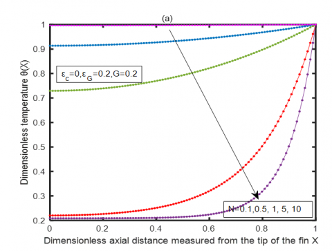
In Figure 2, as N increases, the temperature θ(X) decreases more sharply, indicating enhanced heat dissipation along the fin. For lower values of N, the temperature remains relatively higher throughout the fin length. As the nonlinearity parameter N increases, the temperature profiles become steeper, especially near the base region, suggesting stronger nonlinear effects. The figures demonstrate that higher N values significantly accelerate the cooling process. Throughout the analysis, the parameters εc, εG, and G are kept constant.
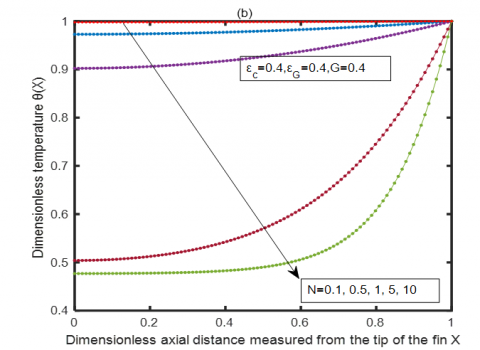
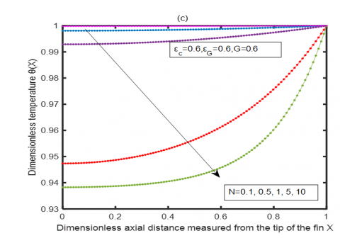
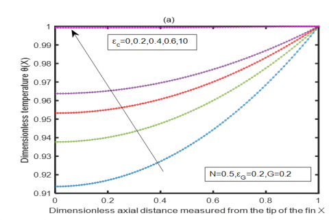
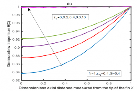
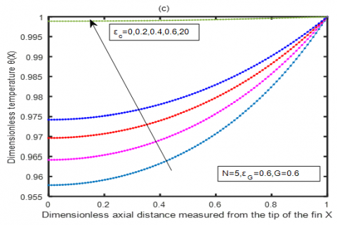
Figure 3(a)-(c) presents the influence of the parameter εc on the dimensionless temperature distribution θ(X) and the dimensionless base temperature ratio θ(X) along the fin length for different conditions. In Figures 3(a) and 2(b), as εc increases, the temperature profiles θ(X) show a more rapid decline along the axial distance, indicating greater thermal conductivity effects. Each curve shifts downward with increasing εc, meaning higher values of εc enhance the cooling of the fin. Figure 3(c) focuses on the dimensionless base temperature ratio, which also decreases more noticeably with higher εc, emphasizing its significant role in thermal performance. Throughout the study, the parameters N, εG, G are fixed to illustrate the isolated effect of εc.
Figure 3. Effect of parameter εc on the temperature distribution function θ(X) for various parameters N, εG, G when εc=0, 0.2, 0.4, 0.6
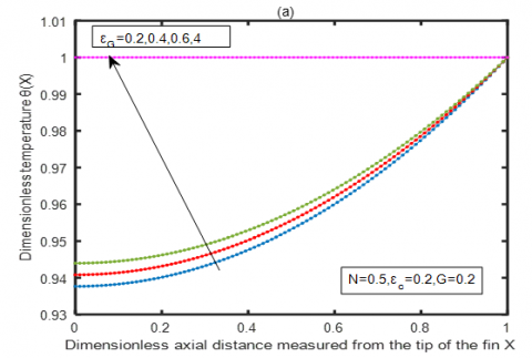
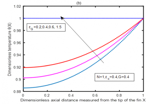
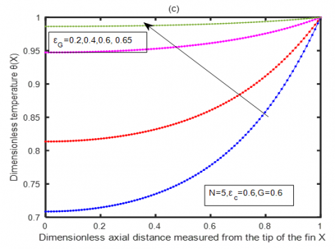
Figure 4(a)-(c) illustrates the effect of the parameter εG on the dimensionless temperature distribution θ(X) along the axial distance of the fin for various fixed values of N, εc, G. In each subfigure, an increase in εc leads to a noticeable reduction in the temperature θ(X) across the fin, highlighting the significant role of surface emissivity in enhancing heat loss. In Figures 4(a) and 4(b), higher εG values cause steeper temperature drops, especially near the base. Figure 4(c) further confirms this trend with a stronger cooling effect as εG rises. These results clearly show that increasing εG enhances radiative heat transfer, leading to lower temperature profiles along the fin length.
Figure 4. Effect of parameter εG on the temperature distribution function θ(X) for various parameters N, εc, G when εG=0.2, 0.4, 0.6
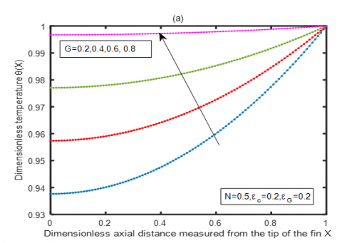
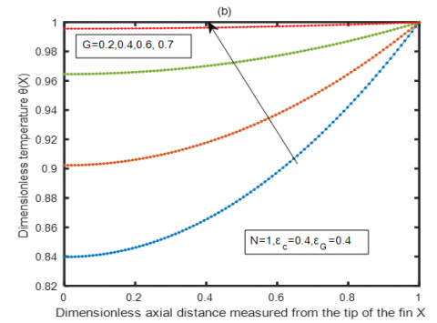
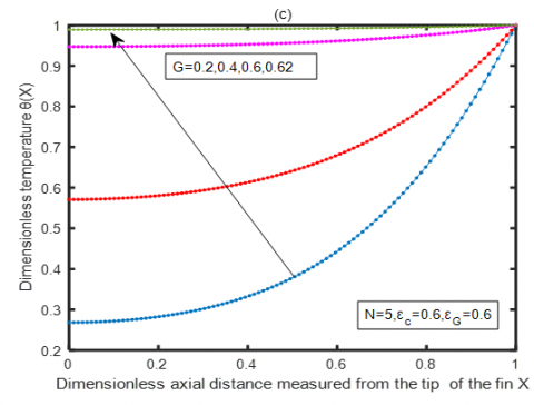
Figure 5(a)-(c) displays the effect of the parameter G on the dimensionless temperature distribution θ(X) along the axial distance from the tip of the fin for different fixed values of N, εc, εG. As shown, increasing G leads to a pronounced decrease in the temperature θ(X) along the fin, indicating enhanced convective heat loss. Each subfigure demonstrates that higher values of G result in steeper temperature gradients, especially closer to the fin base. The influence of G is consistent across the different cases, with G=0.6 producing the lowest temperature profiles. These results emphasize that increasing G significantly boosts the fin’s cooling efficiency by strengthening the convective heat transfer mechanisms.
Figure 5 illustrates how temperature changes for different values of other factors in relation to the heat generation number G. The temperature rises in proportion to the internal heat generating number. The temperature gradient at the bottom of the fin for each curve in Figures 3-5 shows that the fin is absorbing heat from the main surface and releasing this heat into the surrounding area, along with the heat it generates on its own. The intended function of the fin may be undermined by an unfavourable situation where some energy transfers to the main surface rather than dissipating to the sink due to excessive internal heat generation.
Figure 5. Effect of parameter G on temperature distribution function θ(X) for various parameters N, εc, εG when G=0.2, 0.4, 0.6
The local fin temperature rises when the parameters G, εG, and εc rise, according to a comparison of Figures 3-5. The rise in internal heat production G is the cause of this increase. A greater fin temperature is produced as a consequence of the rise in parameter εG which suggests that heat production is a stronger dependence of the local fin temperature. An increase in εc indicates that the fin's thermal conductivity is more strongly influenced by the local temperature. The temperature profile gets flatter with increasing temperatures across the fin due to the fin's increased thermal conductivity, which causes heat transfer with fewer temperature gradients.
In conclusion, the thermal analysis of convective fins, both analytically and numerically, demonstrates the effectiveness of using Taylor series expansions to tackle nonlinear heat transfer problems. The parameters significantly impact the heat transfer process, particularly near the base of the fin, where changes in thermal conductivity and intensified heat generation lead to deviations from the traditional linear temperature distribution.
As the base temperature increases, the temperature-dependent parameters—especially the rise in thermal conductivity—create more complex heat transfer patterns along the fin, which are effectively captured by the analytical model. This sensitivity to material properties emphasizes the critical role that temperature-dependent variations play in determining the thermal efficiency and performance of the fin. The results suggest that the Taylor series-based method is not only accurate but also adaptable to varying thermal conditions, offering a valuable tool for optimizing thermal management systems, such as heat exchangers, where controlling material properties can lead to substantial improvements in efficiency.
This analytical approach presents a promising alternative to purely numerical methods, balancing computational efficiency with high accuracy. Furthermore, the method’s ability to handle temperature-dependent parameters makes it a versatile tool that could be applied to a wide range of heat transfer systems, from simple fins to more complex geometries and boundary conditions, enhancing its applicability in the design and optimization of advanced thermal systems.
|
h |
convection heat transfer coefficient, W/m2K |
|
k |
thermal conductivity, W/mK |
|
P |
fin perimeter, m |
|
T |
local fin temperature, K |
|
G |
dimensionless generation number |
|
N |
dimensionless Fin parameter |
|
X |
dimensionless axial distance measured from the tip of the fin |
|
$k_0$ |
thermal conductivity at zero temperature, W/mK |
|
q* |
internal rate of heat generation, W/m3 |
|
$q_{\infty}^*$ |
internal rate of heat generation at sink temperature $T_{\infty}$, W/m3 |
|
$T_b$ |
fin base temperature, K |
|
$T_{\infty}$ |
sink temperature for convection, K |
|
Greek symbols |
|
|
$\beta$ |
thermal conductivity, K-1 |
|
$\varepsilon$ |
internal heat generation parameter, K-1 |
|
$\varepsilon_c$ |
dimensionless thermal conductivity parameter |
|
$\varepsilon_G$ |
dimensionless internal heat generation parameter |
|
$\theta$ |
dimensionless temperature, $\left(T-T_{\infty}\right) /\left(T_b-T_{\infty}\right)$ |
[1] Kraus, A.D., Aziz, A., Welty, J., Sekulic, D.P. (2001). Extended surface heat transfer. Applied Mechanics Reviews, 54(5): B92. https://doi.org/10.1115/1.1399680
[2] Aziz, A., Bouaziz, M.N. (2011). A least squares method for a longitudinal fin with temperature dependent internal heat generation and thermal conductivity. Energy Conversion and Management, 52(8-9): 2876-2882. http://doi.org/10.1016/j.enconman.2011.04.003
[3] Razani, A., Ahmadi, G. (1977). On optimization of circular fins with heat generation. Journal of the Franklin Institute, 303(2): 211-218. https://doi.org/10.1016/0016-0032(77)90048-5
[4] Ünal, H.C. (1987). Temperature distributions in fins with uniform and non-uniform heat generation and non-uniform heat transfer coefficient. International Journal of Heat and Mass Transfer, 30(7): 1465-1477. https://doi.org/10.1016/0017-9310(87)90178-5
[5] Shouman, A.R. (1968). Nonlinear heat transfer and temperature distribution through fins and electric filaments of arbitrary geometry with temperature-dependent properties and heat generation. National Aeronautics and Space Administration, TND-4257: 1968.
[6] Kundu, B. (2007). Performance and optimum design analysis of longitudinal and pin fins with simultaneous heat and mass transfer: Unified and comparative investigations. Applied Thermal Engineering, 27(5-6): 976-987. https://doi.org/10.1016/j.applthermaleng.2006.08.003
[7] Domairry, G., Fazeli, M. (2009). Homotopy analysis method to determine the fin efficiency of convective straight fins with temperature-dependent thermal conductivity. Communications in Nonlinear Science and Numerical Simulation, 14(2): 489-499. http://doi.org/10.1016/j.cnsns.2007.09.007
[8] Inc, M. (2008). Application of homotopy analysis method for fin efficiency of convective straight fins with temperature-dependent thermal conductivity. Mathematics and Computers in Simulation, 79(2): 189-200. https://doi.org/10.1016/j.matcom.2007.11.009
[9] Ganji, D.D., Ganji, Z.Z., Ganji, D.H. (2011). Determination of temperature distribution for annular fins with temperature dependent thermal conductivity by HPM. Thermal Science, 15(s1): 111-115. http://doi.org/10.2298/TSCI11S1111G
[10] Aziz, A., Khani, F. (2011). Convection–radiation from a continuously moving fin of variable thermal conductivity. Journal of the Franklin Institute, 348(4): 640-651. http://doi.org/10.1016/j.jfranklin.2011.01.008
[11] Bouaziz, M.N., Aziz, A. (2010). Simple and accurate solution for convective–radiative fin with temperature dependent thermal conductivity using double optimal linearization. Energy Conversion and Management, 51(12): 2776-2782. http://doi.org/10.1016/j.enconman.2010.05.033
[12] Kumar, R.S., Sowmya, G., Kumar, R. (2023). Execution of probabilists’ Hermite collocation method and regression approach for analyzing the thermal distribution in a porous radial fin with the effect of an inclined magnetic field. The European Physical Journal Plus, 138(5): 1-19. https://doi.org/10.1140/epjp/s13360-023-03986-3
[13] Ananth Subray, P.V., Hanumagowda, B.N., Varma, S.V.K., Zidan, A.M., Kbiri Alaoui, M., Raju, C.S.K., Junsawang, P. (2022). Dynamics of heat transfer analysis of convective-radiative fins with variable thermal conductivity and heat generation: Differential transformation method. Mathematics, 10(20): 3814. https://doi.org/10.3390/math10203814
[14] Gireesha, B.J., Sowmya, G., Srikantha, N. (2022). Heat transfer in a radial porous fin in the presence of magnetic field: A numerical study. International Journal of Ambient Energy, 43(1): 3402-3409. https://doi.org/10.1080/01430750.2020.1831599
[15] Liu, L., Qu, D., Zhang, J., Cao, H., Tao, G., Deng, C. (2024). Modeling of workpiece temperature suppression in high-speed dry milling of UD-CF/PEEK considering heat partition and jet heat transfer. Frontiers of Mechanical Engineering, 19(5): 30. https://doi.org/10.1007/s11465-024-0801-7
[16] Zhou, J.K. (1986). Differential Transformation Method and its Application for Electrical Circuits. Wuhan, China: Huazhong University Press.
[17] Ghafoori, S., Motevalli, M., Nejad, M.G., Shakeri, F., Ganji, D.D., Jalaal, M. (2011). Efficiency of differential transformation method for nonlinear oscillation: Comparison with HPM and VIM. Current Applied Physics, 11(4): 965-971. http://doi.org/10.1016/j.cap.2010.12.018
[18] Hassan, I.A.H. (2008). Application to differential transformation method for solving systems of differential equations. Applied Mathematical Modelling, 32(12): 2552-2559. https://doi.org/10.1016/j.apm.2007.09.025
[19] Abazari, R., Abazari, M. (2012). Numerical simulation of generalized Hirota–Satsuma coupled KdV equation by RDTM and comparison with DTM. Communications in Nonlinear Science and Numerical Simulation, 17(2): 619-629. http://doi.org/10.1016/j.cnsns.2011.05.022
[20] Rashidi, M.M., Laraqi, N., Sadri, S.M. (2010). A novel analytical solution of mixed convection about an inclined flat plate embedded in a porous medium using the DTM-Padé. International Journal of Thermal Sciences, 49(12): 2405-2412. http://doi.org/10.1016/j.ijthermalsci.2010.07.005
[21] Abbasov, T., Bahadir, A.R. (2005). The investigation of the transient regimes in the nonlinear systems by the generalized classical method. Mathematical Problems in Engineering, 2005(5): 503-519. http://doi.org/10.1155/MPE.2005.503
[22] Balkaya, M., Kaya, M.O., Sağlamer, A. (2009). Analysis of the vibration of an elastic beam supported on elastic soil using the differential transform method. Archive of Applied Mechanics, 79: 135-146. http://doi.org/10.1007/s00419-008-0214-9
[23] Borhanifar, A., Abazari, R. (2011). Exact solutions for non-linear Schrödinger equations by differential transformation method. Journal of Applied Mathematics and Computing, 35: 37-51. http://doi.org/10.1007/s12190-009-0338-2
[24] Moradi, A., Ahmadikia, H. (2010). Analytical solution for different profiles of fin with temperature-dependent thermal conductivity. Mathematical Problems in Engineering, 2010(1): 568263. http://doi.org/10.1155/2010/568263
[25] Moradi, A. (2011). Analytical solution for fin with temperature dependent heat transfer coefficient. International Journal of Engineering and Applied Sciences, 3(2): 1-12.
[26] Kundu, B., Barman, D., Debnath, S. (2008). An analytical approach for predicting fin performance of triangular fins subject to simultaneous heat and mass transfer. International journal of refrigeration, 31(6): 1113-1120. http://doi.org/10.1016/j.ijrefrig.2008.01.007
[27] Hatami, M., Ganji, D.D. (2014). Thermal behavior of longitudinal convective–radiative porous fins with different section shapes and ceramic materials (SiC and Si3N4). Ceramics International, 40(5): 6765-6775. http://doi.org/10.1016/j.ceramint.2013.11.140
[28] Hatami, M., Ganji, D.D. (2014). Thermal and flow analysis of microchannel heat sink (MCHS) cooled by Cu–water nanofluid using porous media approach and least square method. Energy Conversion and Management, 78: 347-358. https://doi.org/10.1016/j.enconman.2013.10.063
[29] Hatami, M., Ganji, D.D. (2014). Investigation of refrigeration efficiency for fully wet circular porous fins with variable sections by combined heat and mass transfer analysis. International Journal of Refrigeration, 40: 140-151. https://doi.org/10.1016/j.ijrefrig.2013.11.002
[30] Hatami, M., Ganji, D.D. (2013). Thermal performance of circular convective–radiative porous fins with different section shapes and materials. Energy Conversion and Management, 76: 185-193. http://doi.org/10.1016/j.enconman.2013.07.040
[31] Hatami, M., Hasanpour, A., Ganji, D.D. (2013). Heat transfer study through porous fins (Si3N4 and AL) with temperature-dependent heat generation. Energy Conversion and Management, 74: 9-16. http://doi.org/10.1016/j.enconman.2013.04.034
[32] Ananthaswamy, V., Sivasankari, S. (2024). A mathematical study on non-linear temperature-dependent thermal conductivity. Journal of Applied Mathematics and Computational Mechanics, 23(2): 5-18. http://doi.org/10.17512/jamcm.2024.2.01
[33] Ghasemi, S.E., Hatami, M., Ganji, D.D. (2014). Thermal analysis of convective fin with temperature-dependent thermal conductivity and heat generation. Case Studies in Thermal Engineering, 4: 1-8. https://doi.org/10.1016/j.csite.2014.05.002