© 2018 IIETA. This article is published by IIETA and is licensed under the CC BY 4.0 license (http://creativecommons.org/licenses/by/4.0/).
OPEN ACCESS
This paper integrates the particle filtering (PF) algorithm with the Lie group theory into an innovative video target tracking algorithm. This algorithm describes the target features with covariance matrix, and expresses the position and shape changes of the target, considering the spatial and temporal statistics. There are three innovations in this research: the state equation and observation equation of the PF under the Riemannian manifold were derived, the geodesic distance under the Riemannian manifold was defined, and a novel PF framework was developed based on the Lie group manifold and applied to video target tracking. The proposed algorithm was tested in the tracking experiments on two video targets. The experimental results show that, compared to the traditional PF algorithm based on the Euler vector space (EVPF), the proposed algorithm enjoys good robustness and tracking effect despite the particle degradation, target occlusion and target deformation. The research findings provide a new alternative for various applications based on target tracking.
target tracking, lie group, riemannian manifold, particle filtering (PF)
In video target tracking, the moving target in a video sequence is detected, extracted, recognized and tracked to obtain their motion states (e.g. position, velocity and acceleration) and trajectory parameters. On this basis, the behaviours of the moving target are understood through further analysis and processing of the obtained data, laying the basis for more advanced tasks. With the recent, overall development of computer technology, the tracking of a single target or multiple targets in the video sequence has become a research hotspot in the field of computer vision, which involves various cutting-edge techniques like image processing, pattern recognition, artificial intelligence, automation control and signal treatment. So far, video target tracking has been widely applied in such fields as missile guidance, intelligent traffic monitoring (Pai et al., 2004), mobile robot visual navigation, human-computer interaction (Newcombe et al., 2011), auxiliary diagnosis (Rabbi and Ullah, 2013) and 3D scene reconstruction.
The Lie group manifold is adopted in many target tracking and matching algorithms. For instance, Wang et al., (2010) puts forward a novel tracking algorithm for the non-rigid target, in which each target is expressed as a feature covariance matrix; this algorithm, with a few dimensions, can capture the spatial and statistical features of the region while depicting the relationship between the pixels, and can effectively integrate different types of features and attributes. Based on particle filtering (PF), Li et al., (2010) proposes a video tracking method capable of gradual self-correction on affine groups, which takes the scale-invariant feature transform as the basic feature descriptor. Wu et al., (2009) presents a tracking method that gradually increases the covariance tensor on Riemannian manifold; this method describes the deformation of the target by affine transformation, and effectively eliminates background interference using the PF framework. Targeting stereo matching, Gu and Zhou, (2008) creates a novel similarity measure under the Riemannian metric: the point information is depicted by structural tensors, and then the similarity is measured by the distance between the structural tensors, which equals the geodesic distance on the Riemannian manifold because the structural tensors obey this manifold.
In light of the above algorithms, this paper develops a novel video target tracking algorithm based on Lie group manifold and PF. Firstly, the foreground target features were constructed in the Lie group space. Then, the target was described and tracked by the manifold theory. Finally, the proposed algorithm was applied to a simulation experiment, and proved to be capable of tracking the target under particle degradation, target occlusion and target deformation. Suffice it to say that this research provides a robust tracking method under complex background.
The remainder of this paper is organized as follows: Section 2 introduces the theoretical basis of the proposed algorithm; Section 3 discusses the feature representation method and extraction method of the tracking target; Section 4 constructs the framework of the target tracking algorithm through the combination of PF and a popular theory; Section 5 analyses the experimental results; Section 6 wraps up this paper with some meaningful conclusions.
Video target tracking can be viewed as the estimation of the motion states of the target. Kalman filtering (KF) (Pedersen, 2013; Bourmaud et al., 2015; Sipos, 2008) and PF (Kwon et al., 2007; Choi and Christensen, 2012) are two poplar methods to estimate the motion states. The translation, rotation, expansion and deformation of a target in the video sequence can be represented by projective transformation. With the aid of the mathematical tool of differential manifold, the projective transformation of the target in the image can be constructed into a Lie group, taking the transformation parameters as state variables. In this way, the state transfer model can be set up on the Lie group, and combined with the PF algorithm framework to realize state estimation.
2.1. Lie group and lie algebra
The Lie group is a group of finite-dimensional smooth manifolds, also known as differential manifolds, with geometrically symmetric smooth group operations, in which the multiplication and inversion satisfy the smooth mapping on a pair of group elements. Simply speaking, the Lie group is a differentiable smooth manifold.
Each Lie group corresponds to a Lie algebra whose vector space is the tangent space of the Lie group manifold at the unit element. The Lie algebra describes the local properties of the Lie group. The Lie group and Lie algebra are connected by exponential mapping (Hall, 2004).
A Lie algebra, consisting of a set V, a number field F and a binary operation [,], should carry the following properties:
(1) Closed: $\forall \mathrm { X } , \mathrm { Y } \in \mathrm { V } , [ \mathrm { X } , \mathrm { Y } ] \in \mathrm { V }$ .
(2) Bilinear: $\forall \mathrm { X } , \mathrm { Y } , \mathrm { Z } \in \mathrm { V } , \mathrm { a } , \mathrm { b } \in \mathrm { F }$ such that $[ \mathrm { aX } + \mathrm { bY } , \mathrm { Z } ] = \mathrm { a } [ \mathrm { X } , \mathrm { Z } ] + \mathrm { b } [ \mathrm { Y } , \mathrm { Z } ] , [ \mathrm { Z } ,$ $\mathrm { aX } + \mathrm { bY } ] = \mathrm { a } [ \mathrm { Z } , \mathrm { X } ] + \mathrm { b } [ \mathrm { Z } , \mathrm { Y } ] .$
(3) Reflexive: $\forall \mathrm { X } \in \mathrm { V } , [ \mathrm { X } , \mathrm { X } ] = 0$
(4) Jacobian equivalent: $\forall \mathrm { X } , \mathrm { Y } , \mathrm { Z } \in \mathrm { V } , [ \mathrm { X } , [ \mathrm { Y } , \mathrm { Z } ] ] + [ \mathrm { Z } , [ \mathrm { X } , \mathrm { Y } ] ] + [ \mathrm { Y } , [ \mathrm { Z } , \mathrm { X } ] ] = 0$
The binary operation is called the Lie bracket.
The general linear group GL(n) is a set of n×n invertible matrices with conventional matrix operations. Among them, the set of matrices with a determinant of 1 forms a special linear group SL(n). Since the target deformation is continuous, the homography matrix satisfies the condition of SL(3) and becomes a Lie group, after normalization. The corresponding Lie algebra and base are denoted as sl(3) and $A _ { i } , i \in [ 1,8 ]$, respectively. The details are as follows:
$A _ { 1 } = \left[ \begin{array} { c c c } { 1 } & { 0 } & { 0 } \\ { 0 } & { - 1 } & { 0 } \\ { 0 } & { 0 } & { 0 } \end{array} \right] , A _ { 2 } = \left[ \begin{array} { c c c } { 0 } & { 1 } & { 0 } \\ { 0 } & { 0 } & { 0 } \\ { 0 } & { 0 } & { 0 } \end{array} \right] , A _ { 3 } = \left[ \begin{array} { c c c } { 0 } & { 0 } & { 0 } \\ { 1 } & { 0 } & { 0 } \\ { 0 } & { 0 } & { 0 } \end{array} \right] , A _ { 4 } = \left[ \begin{array} { c c c } { 0 } & { 0 } & { 0 } \\ { 0 } & { 1 } & { 0 } \\ { 0 } & { 0 } & { - 1 } \end{array} \right]$
$A _ { 5 } = \left[ \begin{array} { c c c } { 0 } & { 0 } & { 1 } \\ { 0 } & { 0 } & { 0 } \\ { 0 } & { 0 } & { 0 } \end{array} \right] , A _ { 6 } = \left[ \begin{array} { c c c } { 0 } & { 0 } & { 0 } \\ { 0 } & { 0 } & { 1 } \\ { 0 } & { 0 } & { 0 } \end{array} \right] , A _ { 7 } = \left[ \begin{array} { c c c } { 0 } & { 0 } & { 0 } \\ { 0 } & { 0 } & { 0 } \\ { 1 } & { 0 } & { 0 } \end{array} \right] , A _ { 8 } = \left[ \begin{array} { c c c } { 0 } & { 0 } & { 0 } \\ { 0 } & { 0 } & { 0 } \\ { 0 } & { 1 } & { 0 } \end{array} \right]$ (1)
2.2. PF
The PF is a statistical filtering method based on Monte-Carlo method and recursive Bayesian estimation. In essence, the PF approximates the probability density function by the values of a group of random samples (particles) propagating in the state space, and replaces the integral calculation with the sample mean, thereby yielding the minimum variance estimate of the system state (Kwon et al., 2014).
Compared with the KF, the PF can be applied to any nonlinear non-Gaussian stochastic system that can be represented by a state space model, and can accurately approximate the optimal estimation (Kwon et al., 2014). As a result, the KF algorithm framework has been extensively implemented in video target tracking systems. The basic steps of the PF algorithm are as follows:
(1) Initializing the particle set: Generate the particle set $\left\{ x _ { 0 } ^ { i } \right\} _ { i = 1 } ^ { N }$ from the prior probability x0, in which each particle weighs 1/N.
(2) Updating weights: Select the weights through importance sampling. The weight of particle i at time k can be updated by the following formula:
$\omega _ { k } ^ { i } \propto \frac { p \left( Z _ { k } | x _ { k } ^ { i } \right) p \left( x _ { k } ^ { i } | x _ { k - 1 } ^ { i } \right) p \left( x _ { 0 : k - 1 } ^ { i } | z _ { 1 : k - 1 } \right) } { q \left( x _ { k } ^ { i } | x _ { 0 : k - 1 } ^ { i } , Z _ { 1 : k } \right) q \left( x _ { 0 : k - 1 } ^ { i } | z _ { 1 : k - 1 } \right) } = \omega _ { k - 1 } ^ { i } \frac { p \left( z _ { k } | x _ { k } ^ { i } \right) p \left( x _ { k } ^ { i } | x _ { k - 1 } ^ { i } \right) } { q \left( x _ { k } ^ { i } | x _ { 0 : k - 1 } ^ { i } , Z _ { 1 : k } \right) }$ (2)
Taking the prior probability density function as the importance density function, formula (2) can be simplified to:
$\omega _ { k } ^ { i } = \omega _ { k - 1 } ^ { i } p \left( z _ { k } | x _ { k } ^ { i } \right) ( i = 1,2 , \cdots , N )$ (3)
After weight normalization, we have:
$\omega _ { k } ^ { i } = \omega _ { k } ^ { i } / \sum _ { i = 1 } ^ { N } \omega _ { k } ^ { i }$ (4)
The least mean squares of unknown parameter x at time k can be estimated as:
$\widetilde { x _ { k } } \approx \sum _ { i = 1 } ^ { N } \omega _ { k } ^ { i } x _ { k } ^ { i }$ (5)
(3) Resampling: If the particles are severely degraded, resampling is needed to obtain a new set of particles $\left\{ x _ { k } ^ { i } \right\} _ { i = 1 } ^ { N }$.
(4) Predicting the state at time k+1: Predict the unknown parameter $\chi _ { k + 1 } ^ { i }$ by the sate equation, and go to Step (2).
Single feature-based tracking is easy to fail when the target deforms significantly, encounters intense illumination changes, or suffers from partial or complete occlusion. Therefore, this paper takes the feature covariance matrix as the target feature to be tracked. In general, the tracking target is limited to the rectangular area R. The basic principle of the feature covariance matrix is as follows: Let M*N be the size of area R, and F={fi | i=1,2,…,M*N} be the set of d-dimensional vectors corresponding to the pixels in area R; then, the d-dimensional feature covariance matrix CR of the area R can be expressed as:
$C _ { R } = \frac { 1 } { M * N } \sum _ { i = 1 } ^ { M * N } \left( f _ { i } - \mu _ { R } \right) \left( f _ { i } - \mu _ { R } \right) ^ { T }$ (6)
where $\mu _ { R } = \frac { 1 } { M * N } \sum _ { i = 1 } ^ { M * N } f _ { i }$ is the vector mean. The features like position, grayscale and gradient can be used together to ensure the robustness of the feature against illumination changes. Here, the feature vector is defined as $f _ { i } =$ $\left[ x , y , I , \left| I _ { x } \right| , \left| I _ { y } \right| , \Delta , \left| I _ { x x } \right| , \left| I _ { y y } \right| \right]$ , where $x , y$ are the coordinates of pixel position; $I$ is the grayscale; $\left| I _ { x } \right| , \left| I _ { y } \right| , \left| I _ { x x } \right|$ and $\left| I _ { y y } \right|$ are the first-order gradient in the $x$ direction, the first-order gradient in the y direction, the second-order gradient in the x direction and the second-order gradient in the y direction, respectively; $\Delta = \sqrt { I _ { x } ^ { 2 } + I _ { y } ^ { 2 } }$ is the mode of the first-order gradient. The CR thus calculated is a real symmetric positive definite matrix of 8*8 elements, and independent of the size of the target area (Wang et a., 2010).
The covariance matrix is a Riemannian manifold rather than an Euler space. The Riemannian manifold is a non-compact Lie group with no double-invariant Riemannian metric, and its exponential mapping is no longer a geodesic. Thus, the metric structure should be redefined on the covariance matrix manifold. In most cases, the length of the vector on the tangent space of a point on the manifold is defined as $\| \mathrm { U } \| = < \mathrm { U } , \mathrm { U } > ^ { \frac { 1 } { 2 } } ,$ with $< \therefore >$ being the inner product of the tangent space, i.e. the Riemann metric. The two covariance matrices on the manifold are denoted as X and Y, respectively. This paper adopts the Riemann metric defined in Reference (Porikli et al., 2006):
$< y , z > _ { X } = \operatorname { tr } \left( X ^ { - 1 / 2 } y X ^ { - 1 } z X ^ { - 1 / 2 } \right)$ (7)
Then, the distance between two points is:
$d ^ { 2 } ( X , Y ) = \| \mathrm { y } \| _ { X } ^ { 2 } = < y , z > _ { X } = < \log _ { X } Y , \log _ { X } Y > _ { X }$ $= \operatorname { tr } \left( \log ^ { 2 } \left( X ^ { - 1 / 2 } Y X ^ { - 1 / 2 } \right) \right.$ (8)
The target tracking problem was modelled as a hidden Markov model, such that the current state St can be estimated according to the images $I _ { 1 : t } = \left\{ I _ { 1 } , I _ { 2 } , \cdots , I _ { t } \right\}$ observed at different times.
During the tracking process, the shape and position changes of the target can be represented as projective transformation. Correspondingly, the apparent change between two frames of the target can be regarded as the motion of the point corresponding to the feature covariance matrix on the manifold (Choi and Christensen, 2012). Therefore, the target motion model can be depicted by the manifold, while the transformation relationship between two adjacent points can be described by the tangent space of the point on the manifold (Kwon et al., 2014; Porikli et al., 2006). The motion model based on the Riemannian manifold and the tangent space can be rewritten as:
$S _ { t } = S _ { t - 1 } \exp \left( V _ { t - 1 } \right)$ (9)
$V _ { t } = \lambda \left( V _ { t - 1 } - V _ { t - 2 } \right) + \mu _ { t - 1 }$ (10)
where $S _ { t } = \left[ x _ { 1 } , x _ { 2 } \cdots , x _ { 8 } \right]$ are the parameter vectors of projective transformation; $V _ { t }$ is the motion velocity of the target from the state $S _ { t - 1 }$ to state $S _ { t } ,$ that is, the tangent, vector corresponding to the state point $S _ { t - 1 }$ on the manifold. The velocity variation is expressed as a second-order autoregressive model, with $\lambda$ being the autoregressive model parameter and $\mu _ { t - 1 }$ being the Gaussian white noise.
During the tracking process, the latest state estimate at each time was correctly iteratively against the observed data; the probability of each sample (particle) was estimated by measuring the similarity between the observed data and the model. Let $p \left( I _ { t } | S _ { t } \right)$ be the observation of $I _ { t }$ under $S _ { t }$ . Then, an observation model was established as: $p \left( I _ { t } | S _ { t } \right) \propto \exp \left( - a \left\| d ^ { 2 } \left( C ^ { * } , C _ { S _ { t } } \right) \right\| ^ { 2 } \right) ,$ where $C ^ { * }$ is the feature covariance matrix of the target template, and $C _ { S _ { t } }$ is the feature covariance matrix of the target image under the projective transformation $S _ { t }$ .
The weight of each particle was defined as: $\omega _ { t } ^ { j } = \exp \left( - a \left\| d ^ { 2 } \left( C ^ { * } , C _ { S _ { t } } ^ { J } \right) \right\| ^ { 2 } \right) ,$ with $C _ { S _ { t } } ^ { j }$ being the feature covariance matrix corresponding to the candidate point $S _ { t } ^ { j } .$ After normalization, we have $\omega _ { t } ^ { j } = \omega _ { t } ^ { j } / \sum _ { j = 1 } ^ { N } \omega _ { t } ^ { j } ,$ where $N$ is the number of particles.
Two videos were selected and processed by Euler vector space PF algorithm (EVPF) and the proposed algorithm (LMPF), which is based on Lie group manifold and the PF. The tracking effects of the two algorithms were contrasted to verify the effectiveness of the LMPF. In one of the videos, the set of images is featured by a complex background and occluded scenes, and the tracking target (helicopter), a rigid body, has an irregular shape and time-varying postures. In the other video, the background is relatively stable, but the tracking target (footballer) is a non-rigid body. Both algorithms were compiled with Matlab 2015b on a computer (Intel® Core™ i5-7200U; 2.70GHz; 8G). A total of 400 frames were tracked for each video. The number of particles was set to 400, and the area error ratio by the algorithm in Reference (Mei et al., 2006):
AvgAreaError$= \frac { 1 } { n } \sum _ { i = 1 } ^ { n } \frac { | S _ { \text {track} ^ { i } } ^ { i } - S _ { \text {templ} } } { S _ { \text {temp} } }$ (11)
where $n$ is the number of tracked frames; $S _ { \text {track} } ^ { n }$ is the area of the target area tracked by the n-th frame; $S _ { \text {temp} }$ is the area of the target template.
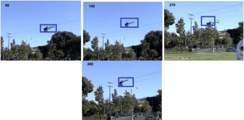
Figure 1. EVPF tracking effect of helicopter.
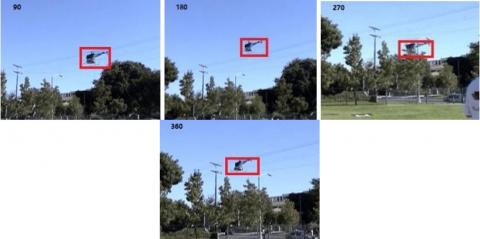
Figure 2. LMPF tracking effect of helicopter.
Figure 3. EVPF tracking effect of footballer.
Figure 4. LMPF tracking effect of footballer.
In the experiment on the first video, each frame has 320×240 pixels and the target template has 55×45 pixels. Figures 1 and 2 respectively display the tracking effects of the EVPF and the LMPF at the 90-th, 180-th, 270-th and 360-th frames. The effects at the 270-th frame show that the EVPF had a large deviation under a complex background and the occlusion of the tracking target, while the proposed algorithm tracked the target well. Under the experimental conditions, the relative error of the EVPF algorithm was 0.237, and that of the proposed algorithm was 0.178. This means the proposed algorithm performs well in the tracking of irregular rigid target under a complex background and occlusions.
In the experiment on the second video, each frame has 480×360 pixels and the target template has 30×55 pixels. Figures 3 and 4 respectively show the tracking effects of the EVPF and the LMPF at the 90-th, 180-th, 270-th and 360-th frames. Through comparison, it is learned that the proposed algorithm outperformed the EVPF when the human body exhibited obvious deformations (the 270-th and the 360-th frames). Under the experimental conditions, the relative error of the EVPF algorithm was 0.197, and that of the proposed algorithm was 0.122. Thus, the proposed algorithm is a better alternative than the traditional EVPF for the tacking of non-rigid target.
This paper puts forward a video target tracking algorithm based on Lie group manifold. Inspired by the PF, the projective transformation was employed to express the position and shape changes of the target, forming the Riemannian manifold. Meanwhile, the covariance matrix was taken as the target feature for tracking. The experimental results demonstrate that the proposed algorithm outperformed the traditional EVPF under particle degradation, target occlusion and target deformation. However, the proposed algorithm only applies to single-target tracking, and does not support real-time tracking due to the features of the PF algorithm. The future research will try to extend the proposed algorithm to multi-target tracking and improve its real-time tracking ability.
This research was jointly supported by the Foundation of Jilin Province Education Department (JJKH20180985KJ) and Foundation of Jilin Provincial Science & Technology Department (20180622006JC, 20170101009JC).
Bourmaud G., Mégret R., Arnaudon M., Giremus A. (2015). Continuous-Discrete Extended Kalman Filter on Matrix Lie Groups Using Concentrated Gaussian Distributions. Journal of Mathematical Imaging & Vision, Vol. 51, No. 1, pp. 209-228. https://doi.org/10.1007/s10851-014-0517-0
Choi C., Christensen H. I. (2012). Robust 3D visual tracking using particle filtering on the special Euclidean group: A combined approach of keypoint and edge features. Sage Publications. https://doi.org/10.1177/0278364912437213
Gu Q., Zhou J. (2008). A novel similarity measure under Riemannian metric for stereo matching. IEEE International Conference on Acoustics, Speech and Signal Processing, pp. 1073-1076. https://doi.org/10.1109/ICASSP.2008.4517799
Hall B. C. (2004). Lie groups, Lie algebras, and representations. An elementary introduction. Springer Berlin, Vol. 659, No. 5, pp. 351. https://doi.org/10.1007/978-0-387-21554-9
Kwon J., Choi M., Park F. C., Changmook C. (2007). Particle filtering on the Euclidean group: framework and applications. Robotica, Vol. 25, No. 6, pp. 725-737. https://doi.org/10.1017/S0263574707003529
Kwon J., Lee H. S., Park F. C., Lee K. M. (2014). A Geometric Particle Filter for Template-Based Visual Tracking. IEEE Transactions on Pattern Analysis & Machine Intelligence, Vol. 36, No. 4, pp. 625-643. https://doi.org/10.1109/TPAMI.2013.170
Kwon J., Lee K. M., Park F. C. (2014). Visual Tracking via Geometric Particle Filtering on the Affine Group with Optimal Importance Functions. Revista Mexicana De Ciencias Geológicas, Vol. 30, No. 1, pp. 80-95. https://doi.org/10.1109/CVPR.2009.5206501
Li M., Chen W., Huang K., Tan T. (2010). Visual tracking via incremental self-tuning particle filtering on the affine group. Computer Vision and Pattern Recognition, pp. 1315-1322. https://doi.org/10.1109/CVPR.2010.5539815
Mei C., Benhimane S., Malis E., Rives P. (2006). Homography-based Tracking for Central Catadioptric Cameras. International Conference on Intelligent Robots and Systems, pp. 669-674. https://doi.org/10.1109/IROS.2006.282553
Newcombe R. A., Lovegrove S. J., Davison A. J. (2011). DTAM: dense tracking and mapping in real-time. Proceedings of IEEE International Conference on Computer Vision. Los Alamitos: IEEE Computer Society Press, pp. 2320-2327. https://doi.org/10.1109/ICCV.2011.6126513
Pai C. J., Tyan H. R., Liang Y. M., Liao H. Y., Chen S. W. (2004). Pedestrian detection and tracking at crossroads. Pattern Recognition, Vol. 37, No. 5, pp. 1025-1034. https://doi.org/10.1016/j.patcog.2003.10.005
Pedersen K. S. (2013). Unscented Kalman Filtering on Riemannian Manifolds. Journal of Mathematical Imaging & Vision, Vol. 46, No. 1, pp. 103-120. https://doi.org/10.1007/s10851-012-0372-9
Porikli F., Tuzel O., Meer P. (2006). Covariance Tracking using Model Update Based on Lie Algebra. Computer Vision and Pattern Recognition, 2006 IEEE Computer Society Conference on, pp. 728-735. https://doi.org/10.1109/CVPR.2006.94
Rabbi I., Ullah S. (2013). A Survey on Augmented Reality Challenges and Tracking. Acta Graphica Journal for Printing Science & Graphic Communications, Vol. 24, No. 1-2, pp. 29-46. https://doi.org/10.1.1.477.3434
Sipos B. J. (2008). Application of the manifold-constrained unscented Kalman filter. Position, Location & Navigation Symposium, pp. 30-43. https://doi.org/10.1109/PLANS.2008.4569967
Wang G., Liu Y., Shi H. (2010). Covariance Tracking via Geometric Particle Filtering. Eurasip Journal on Advances in Signal Processing, No. 1, pp. 1-9. https://doi.org/10.1155/2010/583918
Wu Y., Wang J., Lu H. (2009). Real-Time Visual Tracking via Incremental Covariance Model Update on Log-Euclidean Riemannian Manifold. Pattern Recognition, pp. 1-5. https://doi.org/10.1109/CCPR.2009.5344069