© 2018 IIETA. This article is published by IIETA and is licensed under the CC BY 4.0 license (http://creativecommons.org/licenses/by/4.0/).
OPEN ACCESS
Because different brain diseases, such as hippocampus, accumbens, and thalamus, are closely related with the shape changes of key brain structures. Nuclear Magnetic Resonance (NMR) Image segmentation plays a vital role in brain disease analysis. However, these structures often have no clear contrasted boundaries in brain NMR images, a priori knowledge based on the atlas is required to better complete the segmentation. In this paper, a hybrid intensity and shape characteristic non-rigid registration algorithm, which is suitable for multiple objects segmentation problem, is proposed. Experiment results proved that better results can be obtained when the proposed algorithm is used to segment brain internal structures.
non-rigid registration, brain NMR image, atlas prior, shape knowledge
Image registration technology initially was acted as an image processing method to transform an image into another image (Pluim & Fitzpatrick, 2003). Now it has been widely used in many fields, especially in medical image processing and analysis field. Medical images can be divided into two categories: anatomical imaging mode and functional imaging mode. Anatomical imaging equipment mainly describes the morphology of human tissues and is used to diagnose the pathological changes in the internal tissues of the body, such as X ray, CT tomographic imaging, magnetic resonance imaging, ultrasound imaging, and video images produced by various endoscopes (Lee et al., 2013; Sun & Bin, 2018;). Functional imaging equipment mainly describes metabolic information of human tissues. They can see in the early stages of the disease without structural changes. Early lesions were found by imaging the metabolism function of organs and tissues. The information contained in the two kinds of images is not isolated but complementary. By fusing different modality images, more information can be obtained to understand the overall situation of pathological tissues or organs. The precondition of fusion is the accurate registration of all kinds of image.
In recent years, the application of medical image registration in medical diagnosis and treatment has increased rapidly. Functional magnetic resonance imaging (FMRI) is a safe imaging method, which can be used for functional localization of human brain under completely noninvasive conditions. In FMRI experiments, in order to obtain statistical significance, multiple experiments are needed to obtain multiple time series. So when brain functional images were analyze, it is necessary to register images in time series of brain function imaging to remove the influence of the subjects’ movement in the process of image acquisition. At present, no segmentation algorithm can accurately segment all FMRI images. Therefore, segmentation of brain NMR images has always been a hot topic in medical image segmentation.
Registration is the most flexible and convenient method of image segmentation (Yang & Burger, 1990). It has been widely applied to NMR segmentation and target tracking. In view of the nonlinear relationship between different individuals, non-rigid registration is a reasonable choice. Non-rigid registration technology (Rueckert & Frangi, 2003) belongs to a local registration method. The local registration technique is no longer limited to several global transformations such as rotation, translation and scaling. Instead, it describes all the local details differences between the two data sets, and its spatial transformation has higher degrees of freedom. However, compared with rigid registration, non-rigid registration is not mature, and the registration speed, registration accuracy, and the reasonable evaluation of registration performance still need to be studied in depth.
There are many methods of image registration (Zhang et al., 2006; Shams et al., 2010). According to the difference of the transformation function, they can be classified the following types.
Rigid transformation: The source image can only be globally translated and rotated, and the distance between any two points in the source image remains unchanged before and after transformation.
Usually, 3D rigid body transformation includes three translational operations and three rotation operations. Point (x, y, z) after the rigid transformation, the coordinates become (X, Y, Z), then the function relation of the two coordinates can be expressed as:
$\begin{aligned} \mathrm { X } = & \mathrm { x } \cos ( \varphi ) \cos ( \omega ) + y [ \sin ( \varphi ) \cos ( \theta ) + \cos ( \varphi ) \sin ( \omega ) \sin ( \theta ) ] \\ & + z [ \sin ( \varphi ) \sin ( \theta ) - \cos ( \varphi ) \sin ( \omega ) \cos ( \theta ) ] + p \end{aligned}$
$Y = - x \sin ( \varphi ) \cos ( \omega ) + y [ \cos ( \varphi ) \cos ( \theta ) - \sin ( \varphi ) \sin ( \omega ) \sin ( \theta ) ]$ $+ z [ \cos ( \varphi ) \sin ( \theta ) + \sin ( \varphi ) \sin ( \omega ) \cos ( \theta ) ] + q$
$\mathrm { Z } = \mathrm { x } \sin ( \omega ) - y \cos ( \omega ) \sin ( \theta ) + z \cos ( \omega ) \cos ( \theta ) + r$
where p, q, r represents the translation parameters along the X axis, the Y axis and the Z axis. $\theta , \omega , \varphi$ represents the angle of rotation around the X axis, the Y axis, and the Z axis.
Affine transformation: The source image can be globally translated, rotated, zoomed and cut. The straight line is mapped into a straight line, and the parallelism of the straight line remains unchanged after mapping, but the angle between the intersecting lines can be changed. The general form of affine transformation contains twelve parameters, and its expressions are as follows:
$\begin{aligned} X & = a _ { 1 } x + a _ { 2 } y + a _ { 3 } z + a _ { 4 } \\ Y & = b _ { 1 } x + b _ { 2 } y + b _ { 3 } z + b _ { 4 } \\ Z & = c _ { 1 } x + c _ { 2 } y + c _ { 3 } z + c _ { 4 } \end{aligned}$
Projection transformation: After transformation, the line is mapped into a straight line, but the parallel or intersecting relations between the lines after mapping can be changed.
Projection transformation is the most general linear transformation, which contains 15 parameters, and its expression is as follows:
$X = \left( a _ { 1 } x + a _ { 2 } y + a _ { 3 } z + a _ { 4 } \right) / ( m x + n y + p z + 1 )$
$Y = \left( b _ { 1 } x + b _ { 2 } y + b _ { 3 } z + b _ { 4 } \right) / ( m x + n y + p z + 1 )$
$Z = \left( c _ { 1 } x + c _ { 2 } y + c _ { 3 } z + c _ { 4 } \right) / ( m x + n y + p z + 1 )$
Elastic transformation: It is also called non-rigid transformation. After mapping, a line can be turned into a curve. Non-rigid transformation can be used to describe the nonlinear distortion introduced in the imaging process. The most common application is the registration of allogeneic medical images, it is used to describe the nonlinear differences between individual organisms. Non-rigid medical image registration algorithms can be divided into three categories: feature-based registration algorithm, gray-scale-based registration algorithm and combined algorithm of feature and gray-scale.
Feature-based registration algorithm firstly needs to extract appropriate and representative data from each matching dataset. Then, these features are parameterized and matched with the corresponding features in the target data. The features used in registration are typically typical structures that can express the nature of images, such as extracted image boundaries, external contour lines, epidermis and so on. Because the feature-based registration method directly calculates fewer points, the registration speed is fast. Moreover, the expression of registration is based on the characteristics and the dependence on image pixels is small. The same registration accuracy can be obtained for different modes. However, the accuracy of registration is affected by the feature extraction. If the feature extraction and feature matching are inaccurate, the registration results will be very disturbed. In this class of registration algorithms, registration based on feature points is an important part. The key of registration algorithm based on feature points is how to find the corresponding feature points in the data set, and then search for matching points automatically. Xue et al., (2004) proposed the use of wavelet eigenvectors as the morphological signature of each pixel, to select two corresponding data points. Curve-based registration is another important part of the algorithm. When establishing a deformation field for registration of two image data sets, the use of curves as driving features can achieve greater registration accuracy. Vos et al., (2017) used the threshold method to divide the cerebral cortex and the ventricle system from the MRI data, and then used the iterative closest point algorithm to match the corresponding curve of the target brain image. The third types of characteristics that are often used are surface, which mainly uses the information of the target boundary surface to determine the matching transformation. Thompson & Toga, (1996) proposed a surface-based registration algorithm, which firstly extracts the brain surface model from each dataset. The surface model includes many important functional areas and different tissue structures in three dimensional space and the junctional regions of different brain lobes. Then, the extracted surfaces and curves are reconstructed and matched with the corresponding structures of the target data.
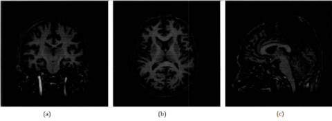
The use of medical NMR images to separate different organs of human brain and analyze the differences in the structure of organs is an important means of clinical diagnosis and identification of brain diseases. The NMR image is a three-dimensional image that provides the structural view of the human brain from three directions. Figure 1 shows a three direction view of a person's brain image, the three directions are called as coronal, axial and sagittal.
There are numerous neurons in the human brain. These neurons are mainly composed of cell bodies and axons. In essence, the brain can be divided into three groups: gray matter, white matter and cerebrospinal fluid. Gray matter is composed of cell bodies, while white matter is the axon, and cerebrospinal fluid is the tissue fluid filled with it. Different water content of tissue is different, the radiofrequency field energy reflects different intensity, it corresponds to different image intensities for the NMR image.
Figure 1. (a) coronal (b) axial (c) sagittal
3.1. Segmentation algorithm based on registration
The registration algorithm based on registration is used to get the spatial transformation of the template image into the target image. Then the space transformation can be used to map the known segmentation results of the template image, which maps atlas information to the target image, and then the segmentation of the target image can be gotten.
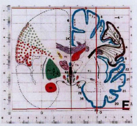
Registration segmentation algorithm firstly depends on the structural information provided by the atlas. The widely used atlas is Talairach and Tournoux atlas, which accurately gives anatomical information of human brain structures (Nowinski & Thirunavuukarasuu, 2009). A slice of the Talairach atlas is shown in Figure 2.
Figure 2. A slice of the Talairach atlas
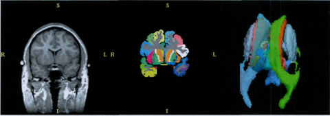
With the development of computer technology, the application of paper atlas has been restricted, and the digital atlas has been gradually developed. Digital atlas can be obtained from individuals or from groups. The most widely used digital atlas is based on individual 3D image segmentation. The atlas contains 265
individual voxels, the size of each voxel is , it contains 150 different brain structures totally. A coronal NMR image of the atlas is shown in Figure 3.Figure 3. A coronal slice of SPL atlas
3.2. Non-rigid registration algorithm based on gray-scale
Image registration can be regarded as an optimization problem. The purpose of optimization is to find the best spatial transformation parameters $T ^ { * }$ according to the similarity targets between the two images.
In the optimization theory, the registration problem can be expressed as: Given the source image $A$ and $B$ , the optimal transformation $T ^ { * }$ is found in the transformation space $\Gamma$ to satisfy the prescribed similarity measure $E _ { \text {sim } } ( B , A \circ T )$ in the best state.
$T ^ { * } = \arg \min _ { T \in \Gamma } \{ E ( T ) \} = \arg \min _ { T \in \Gamma } \left\{ E _ { \operatorname { sim } } ( B , A \circ T ) + E _ { r e g } ( T ) \right\}$
where $E _ { r e q } ( T )$ is regularization function, which is used to ensure that the obtained spatial transformation satisfies certain desirable attributes.
The similarity measure between images is varied, sum of squares difference (SSD) is a basic measure based on gray-scale registration algorithm. The expression of the measure is as follows:
$E _ { \operatorname { sim } } ( B , A \circ T ) = E _ { S S D } ^ { i n t e n s i t y } ( B , A \circ T ) = \frac { 1 } { 2 } \| B - A \circ T \| ^ { 2 }$
The solution obtained by direct optimization in nonparametric space may be unstable. Therefore, it is necessary to add the regularization constraint. The above expression of the measure can be changed as follows:
$E = E _ { \operatorname { sim } } ( B , A \circ T ) + E _ { r e g } ( T ) = E _ { S S D } ^ { i n t e n s i t y } ( B , A \circ T ) + E _ { r e g } ( T )$ $= \frac { 1 } { 2 } \| B - A \circ T \| ^ { 2 } + q \| \Delta T \| ^ { 2 }$
where the regularization constraint is $E _ { r e g } ( T ) = q \| \Delta T \| ^ { 2 }$, parameter q is used to adjust constraint strength.
The regularization constraint is introduced to solve the stability problem of the transformation, but the optimization process becomes more complicated. Based on the Tikhonov regularization method (Fuhry & Reichel, 2012), the closest Tikhonov regularization resolution $\widehat { D }$ to signal D makes the energy function minimum. The energy function can be defined as follows:
$\mathrm { E } ( \widehat { D } ) = \frac { 1 } { 2 } \int \left[ ( \widehat { D } - D ) ^ { 2 } + \sum _ { i = 1 } ^ { \infty } \frac { \sigma ^ { i } } { i ! } \left( \frac { \partial D } { \partial x ^ { i } } \right) ^ { 2 } \right] d x$
The solution of the energy function is
$\widehat { D } = D * h$
where * represents convolution operation.
Fourier transform of filter h is
$\mathrm { G } ( \omega , \sigma ) = \frac { 1 } { \sum _ { i = 0 } ^ { \infty } \frac { \sigma ^ { i } } { i ! } \omega ^ { 2 i } } = e ^ { - \omega ^ { 2 } \sigma }$
3.3. Hybrid intensity and shape characteristic non-rigid registration algorithm
Non-rigid registration algorithm based on gray-scale only uses the gray information of the image. For some applications, the use of gray-scale information alone can’t solve the problem well. For example, in the segmentation of the deep gray matter structure of the brain, if some of the structures to be divided are very close to the target image, and the gray values of these structures are very close, it is difficult to get accurate segmentation. It requires additional information related to the target structure. In general, some suitable feature extraction algorithms will be used to extract the related points, lines and surfaces, which can be used to supplement the deficiency of gray-scale information and to construct a registration algorithm which is mixed with gray-scale and feature information.
In the registration process, the atlas information corresponding to the source image can provide the prior information of the shape and relative position of the region of interest. Therefore, the introduction of shape similarity information on the basis of gray-scale similarity is an effective way to improve registration accuracy.
When a priori shape information is introduced in the gray based registration energy function, an appropriate shape representation method should be required firstly. Implicit distance function representation is more suitable for establishing dense correspondence of shape boundaries. The method can represent the shape of arbitrary dimension and arbitrary topological structure, and it can directly transform the image with the distance of shape. Therefore, in this paper distance function is used to represent shape information and establish similarity measure between shapes.
Shape S divides the image space $\Omega$ into two adjacent areas, $\omega$ represents the area surrounded by $\mathrm { S } , \Omega - \omega$ represents the background area outside the shape. $\Phi _ { S } : \Omega \rightarrow$ $R ^ { + }$ is the distance transform of $\mathrm { S }$ , the minimum distance from any point $\mathrm { p }$ to the shape in the image is d(p, S). The distance graph of the shape is
$\Phi _ { S } ( p ) = \left\{ \begin{array} { c c } { 0 , } & { p \in S } \\ { d ( p , S ) , } & { p \in \omega } \\ { - d ( p , S ) , } & { p \in \Omega - \omega } \end{array} \right.$
where $d ( p , S )$ can use any distance function.
After the distance transformation, the shape information is converted to the gray image with gray-scale as the distance. Based on distance images, a new shape similarity measure is constructed.
$E _ { S S D } ^ { S h a p e } \left( \Phi _ { S } ( A ) , \Phi _ { S } ( A \circ T ) \right) = \frac { 1 } { 2 } \left\| \Phi _ { S } ( A \circ T ) - \Phi _ { S } ( A ) \right\| ^ { 2 }$
where $\Phi _ { S } ( A )$ represents the shape of the target structure in the source image $A ,$ $\Phi _ { S } ( A \circ T )$ represents the shape after deformation of the structure based on space transformation. So, the new energy function is
$\begin{aligned} E _ { \text {new} } = E _ { \text {sim} } ( B , A \circ T ) + E _ { \text {reg} } ( T ) & \\ = & E _ { \text {SSD} } ^ { \text {intensity} } ( B , A \circ T ) + E _ { \text {SSD} } ^ { \text {shape} } \left( \Phi _ { S } ( A ) , \Phi _ { S } ( A \circ T ) \right) + E _ { \text {reg} } ( T ) \end{aligned}$
According to Demons algorithm alternate optimization strategy (Thirion, 1998), the displacement vector corresponding to the gray-scale matching at any point p in the region can be obtained.
$u _ { i n t e n s i t y } = - \frac { ( A \circ T ( p ) - B ( p ) ) } { ( A \circ T ( p ) - B ( p ) ) ^ { 2 } + \| \Delta \mathrm { B } ( \mathrm { p } ) \| ^ { 2 } } \Delta \mathrm { B } ( \mathrm { p } )$
The displacement vector corresponding to the shape matching is
$u _ { \text {shape} } ( p ) = - \frac { \left( \Phi _ { S } ( A \circ T ( p ) ) - \Phi _ { S } ( A ( p ) ) \right) } { \left( \Phi _ { S } ( A \circ T ( p ) ) - \Phi _ { S } ( A ( p ) ) \right) ^ { 2 } + \left\| \Delta \Phi _ { S } ( A ( p ) ) \right\| ^ { 2 } } \Delta \Phi _ { S } ( A ( p ) )$
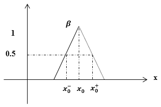
In order to take account of the influence of gray matching and shape matching on image deformation, the balance parameter $\beta \in [ 0,1 ]$ is introduced, it is used to balance the contribution of gray information and shape information to registration. Therefore, the synthetic displacement field at point p is
$u ( p ) = ( 1 - \beta ) u _ { i n t e n s i t y } ( p ) + \beta u _ { s h a p e } ( p )$
In this paper, a simple piecewise linear function shown in Figure 4 is used to adaptively adjust the weights of the parameter knives.
Figure 4. The value of the balance parameter
In Figure 4, x represents the gray value of pixels in the region of interest of the target image. $x _ { 0 }$ represents the average gray value of the target structure area. $x _ { 0 } ^ { + }$ and $x _ { 0 } ^ { - }$ are gray threshold.
In summary, a source image A, a target image B, and an atlas corresponding to the source image are given. The implementation of the proposed algorithm is as follows:
Step 1: Complete the non-brain tissue detachment and correct the inhomogeneous field in the image.
Step 2: Initial registration T1 is achieved by global pre registration of source and target images.
Step 3: Image $A \circ T _ { 1 }$ as a new source image, the Demons algorithm is used to realize the non-rigid registration based on gray-scale to get the nonlinear transformation $T _ { 2}$.
Step 4: The initial segmentation of regioni $Atlas \circ T _ { 1 }\circ T _ { 2 }$ is achieved by atlas mapping.
Step 5: A synthetic shape map for the structure of the pending division is calculated, $T _ { 2}$ is optimized to achieve $T _ { 3}$ by the proposed hybrid intensity and shape characteristic non-rigid registration algorithm in this paper.
Step 6: Through atlas mapping, the segmentation result $Atlas \circ T _ { 1 }\circ T _ {3 }$ of target structure is gotten.
In the experiment, we use the proposed algorithm to divide the caudate nucleus, the putamen and the thalamus from the NMR image of the normal human brain to verify the performance of the algorithm. The template image is provided by the standard weighted NMR image provided by Harvard Medical School and its corresponding atlas.
The algorithm adopts iterative optimization, and the termination condition is the interrelation between the template image and the target image after deformation, or the new image can be used as a deformable template to re-register the number of times to reach the upper limit (3 times in our experiment). In this experiment, the threshold of interrelation number is set as follows: The initial interrelation coefficient between the template image and the target image is $C C _ { 0 } ,$ then the threshold is $C C _ { t } =$ $\left( 1 - C C _ { 0 } \right) / \alpha + C C _ { 0 } ,$ where $\alpha = 1.2 .$.
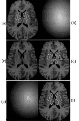
In order to more clearly compare the segmentation performance of different algorithms, Figure 5 shows a set of 2D views of experimental results.
Figure 5. Comparison segmentation results between Demons nor-rigid algorithm and the proposed algorithm
Figure 5 (d) gives the segmentation result of the left putamen. It is only registered with the gray similarity degree registration, and examines the position of the black circle in the picture. Obviously, the result is not ideal. Therefore, if we consider only the gray-scale similarity, it is very likely to fall into the local optimal solution. Figure 5 (e) is a distance map of the deformed left putamen. It can be seen that the shape of the left putamen after deformation is quite different from that of the original shape. Then the shape of the left putamen in the source image is similar to the shape of the left putamen in the target image, and the segmentation result is better under the combined effect of the gray similarity and the shape similarity.
In this paper, the similarity index is used to quantitatively evaluate the segmentation performance of the algorithm. G represents the standard division of a structure. E represents the result of automatic segmentation of the structure, and the definition of the similarity index is as follows.
$\mathrm { KI } = \frac { 2 \times \mathrm { TP } } { 2 \times \mathrm { TP } + \mathrm { FN } + \mathrm { FP } }$
where $\mathrm { TP } = \mathrm { G } \cap \mathrm { E }$ represents correct segmentation rate, $\mathrm { FP } = \overline { G } \cap E$ represents false positive rate, $\mathrm { FN } = \mathrm { G } \cap \overline { E }$ represents false negative rate. The value of $\mathrm { KI }$ is between 0 and $1 .$
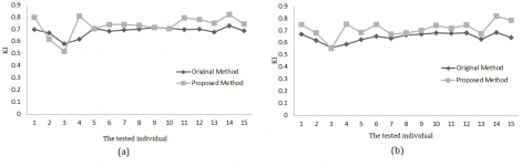
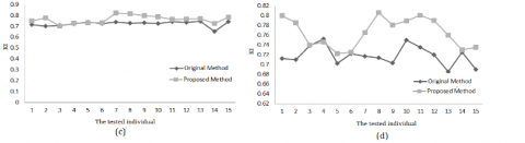
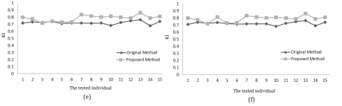
Figure 6. Comparisons of KI values (a) left caudate (b) right caudate (c) left putamen (d) right putamen (e) left thalamus (f) right thalamus
In the experiment, we divided the left and right caudate nucleus, putamen and thalamic structure of 15 normal brain NMR images. Their KI values are calculated and the results are shown in Figure 6.
The relevant statistics are listed in Table 1.
Table 1. The statistical KI value for the target segmentation
|
Tissue |
L-Caudate |
R-Caudate |
L-Putamen |
R-Putamen |
L-Thalamus |
R-Thalamus |
||||||
|
Algorithm |
Pro. |
Ori. |
Pro. |
Ori. |
Pro. |
Ori. |
Pro. |
Ori. |
Pro. |
Ori. |
Pro. |
Ori. |
|
Max |
0.81 |
0.75 |
0.82 |
0.69 |
0.83 |
0.76 |
0.83 |
0.76 |
0.86 |
0.81 |
0.86 |
0.79 |
|
Min |
0.54 |
0.54 |
0.57 |
0.57 |
0.69 |
0.64 |
0.75 |
0.67 |
0.73 |
0.68 |
0.75 |
0.66 |
|
Mean |
0.74 |
0.69 |
0.72 |
0.66 |
0.77 |
0.72 |
0.79 |
0.75 |
0.81 |
0.74 |
0.80 |
0.73 |
|
SD |
0.07 |
0.05 |
0.06 |
0.03 |
0.04 |
0.03 |
0.03 |
0.02 |
0.03 |
0.03 |
0.03 |
0.03 |
|
Pro.: Proposed algorithm Ori.: Original algorithm |
||||||||||||
From Figure 6 and Table 1, we can see that in most cases, the proposed algorithm in this paper is more accurate than the original algorithm. Zijdenbos et al (1994). gave the opinion that $\mathrm { KI } > 0.7$ means automatic segmentation and standard segmentation are very close (Fuhry & Reichel, 2012). In this paper, the KI value of the 15 data segmentation is basically greater than 0.7, it shows that the proposed algorithm has better segmentation performance.
In this paper, the basic principle of non-rigid registration algorithm based on gray-scale is analyzed, and the shape similarity is introduced into the registration energy function, and a new non-rigid registration algorithm combining gray information with shape information is proposed. The proposed algorithm directly uses the gray-scale information of the image to measure the matching degree of the two images by the square of the gray difference, and it is suitable for registration between the same mode images The experiment shows that the new shape similarity terms have beneficial supplement to the missing information of the original algorithm, and have the advantages of simple form, easy understanding and complete automatic processing.
Foundation Items: Shandong Provincial Natural Science Foundation, China (ZR2015FL005).
Fuhry M., Reichel L. (2012). A new Tikhonov regularization method. Numerical Algorithms, Vol. 59, No. 3, pp. 433-45.
Lee W. J., Lee J. Y., Rhim H. (2013). Effect of Respiration On the Registration of US-CT Fusion Imaging for Accurate Localization of Small Focal Hepatic Lesions. Ultrasound in Medicine & Biology, Vol. 39, No. 5, pp. 81-89. https://doi.org/10.1016/j.ultrasmedbio.2013.02.381
Nowinski W. L., Thirunavuukarasuu A. (2009). Quantification of spatial consistency in the Talairach and Tournoux stereotactic atlas. Acta Neurochirurgica, Vol. 151, No. 10, pp. 1207-13. https://doi.org/10.1007/s00701-009-0364-8
Pluim J. P., Fitzpatrick J. M. (2003). Image registration. Medical Imaging IEEE Transactions on, Vol. 22, No. 11, pp. 1341-43. https://doi.org/10.1109/TMI.2003.819272
Rueckert D., Frangi A. F. (2003). Automatic construction of 3-D statistical deformation models of the brain using nonrigid registration. IEEE Trans Med Imaging, Vol. 22, No. 8, pp. 1014-25. https://doi.org/10.1109/TMI.2003.815865
Shams R., Sadeghi P., Kennedy R. A. (2010). A Survey of Medical Image Registration on Multicore and the GPU. Signal Processing Magazine IEEE, Vol. 27, No. 2, pp. 50-60. https://doi.org/10.1109/MSP.2009.935387
Sun G., Bin S. (2018). A new opinion leaders detecting algorithm in multi-relationship online social networks. Multimedia Tools & Applications, Vol. 77, No. 4, pp. 4295–307.
Thirion J. P. (1998). Image matching as a diffusion process: an analogy with Maxwell's demons. Medical Image Analysis, Vol. 2, No. 3, pp. 243-49. https://doi.org/10.1016/S1361-8415(98)80022-4
Thompson P., Toga A. W. (1996). A surface-based technique for warping three-dimensional images of the brain. IEEE Transactions on Medical Imaging, Vol. 15, No. 4, pp. 402-416. https://doi.org/10.1109/42.511745
Vos B. D., Wolterink J., Jong P. D. (2017). ConvNet-Based Localization of Anatomical Structures in 3D Medical Images. IEEE Transactions on Medical Imaging, Vol. 99, pp. 1470-81. https://doi.org/10.1109/TMI.2017.2673121
Xue Z., Shen D., Davatzikos C. (2004). Determining correspondence in 3-D MR brain images using attribute vectors as morphological signatures of voxels. IEEE Transactions on Medical Imaging, Vol. 23, No. 10, pp. 1276-91. https://doi.org/10.1109/TMI.2004.834616
Yang G. Z. (1990). Burger P. Enhancement and segmentation for NMR images of blood flow in arteries. Proc Spie, Vol. 1360, pp. 702-713. https://doi.org/10.1117/12.24257
Zhang J., Zhang J. Z., Jiang W. U. (2006). A survey of medical image registration. Journal of Shaanxi University of Science & Technology, Vol. 2, No.1, pp.1-36.
Zijdenbos A. P., Dawant B. M., Margolin R. A. (1994). Morphometric analysis of white matter lesions in MR images: method and validation. Medical Imaging IEEE Transactions on, Vol. 13, No. 4, pp. 716-24. https://doi.org/10.1109/42.363096