© 2018 IIETA. This article is published by IIETA and is licensed under the CC BY 4.0 license (http://creativecommons.org/licenses/by/4.0/).
OPEN ACCESS
This paper proposes an approach to automatically rank image thresholding methods, where the reference image is unavailable. The ranking is done with respect to reference image, generated by consensus of above methods. It also provides a quantitative performance eva- luation of these thresholding methods. Literature suggests a few performance measures among which F-measure (FM), Modified Hausdorff distance (MHD), Edge mismatch error (EMM), Relative area error (RAE) and Object level consistency error (OCE) are popular. However, cor- relation analysis of these metrics reveal that only FM, MHD and EMM retain non-redundant information. Thus, these three indices are sufficient to measure its performance on different database. The experimental results suggest the technique to be adopted for a particular type of images.
consensus ground truth, edge mismatch error (EMM), F-measure (FM), modified hausdorff distance (HD), object level consistency error (OCE), relative area error (RAE)
In many image processing and computer vision applications like optical character recognition (OCR), document image analysis, scene matching, quality inspection of materials, etc.; separation of object from image background plays an important role. Other applications include map processing (To find the lines, legends and charac- ters), scene processing, feature extraction and object shape detection Sezgin, Sankur, (2004). This technique called as thresholding is a pre-processing step. The use of the binary image output decreases computational load for the overall application.
In this article, a digital image is represented as I (x, y), where (x, y) are the spatial coordinates. If the image is thresholded at gray level 't', then the binary image can be expressed as:
$I_{T}(x, y)=\left\{\begin{array}{l}{0, \text { If } I(x, y) \leq T} \\ {1, \text { If } I(x, y)>T}\end{array}\right.$ (1)
Depending on the context of application the foreground of binary image can be represented by 0 i.e. black, and the background by its highest gray level, i.e. 255 or 1 and viceversa.
According to literature Sezgin and Sankur (2004), all the thresholding techniques can broadly be classified into six different categories (see Table 1). We have conside- red 21 most popular thresholding methods in this article Albuquerque et al. (2004); Brink and Pendock (1996); Huang and Wang (1995); Jawahar et al. (1997); Kapur et al. (1985); Kittler and Illingworth (1986); Li and Lee (1993); Liu and Li (2010); Otsu (1975); Pal and Pal (1989); Ramesh et al. (1995); Ridler and Calvard (1978); Rosenfeld (1984); Rosenfeld and Torre (1983); Sahoo and Arora (2004); Sahoo and Arora (2006); Sahoo et al. (1997); Shaikh et al. (2013); Tsai (1985); Yen et al. (1995). A brief description of each method is given in Table 1.
In order to evaluate the performance of the thresholding methods, several indices have been reported in literature Nitrogiannis et al. (2008); Smith (2010). Most of them utilize ground truth (reference) image Stathis et al. (2008). Sahoo et al. (1988) proposed a subjective method for reference image creation, which is based on visual inspection. This process suffers from inaccuracy in measurement as it re- lies on human observer scores. Moreover, this method is not automatic. Shaikh et al. Shaikh et al. (2013) proposed another method based on majority voting scheme for reference image creation. It may also fail depending on the choice of vote.
We propose a novel approach to automatically generate ground truth for image binarization by consensus of different thresholding methods Fernández-García et al. (2008). The generated reference image is compared with all the binarized images using mean quality score of a few performance indices. Among these performance measures F-measure (FM), Modified Hausdorff distance (MHD), Edge mismatch error (EMM), Relative area error (RAE) and Object level consistency error (OCE) are popular. However correlation analysis of these indices suggest that FM, MHD and EMM retain distinct information. The efficacy of the proposed method (generated reference image) is also examined by randomly selecting the varying number of thresholding techniques. In addition the execution time complexity for real time application is also reported. The experimental results indicate the best method to be selected for particular image type.
Table 1. Broad category of thresholding methods
|
Category |
Thresholding Methods |
Description |
Remark |
|
Histogram shape based methods |
Convex Hull Thresholding Rosenfeld and Torre (1983) Histogram Approximation Ramesh et al. (1995) |
Analyzes the concavities of histogram h(g) Uses a simple function that minimizes sum of square between bi-level function and the histogram of image. |
May not be applicable for the image with varying illumination. |
|
Clustering based methods |
Fuzzy Clustering Thresholding Jawahar et al. (1997); Fuzzy Logic Based Thresholding Jawahar et al. (1997); Iterative Thresholding Ridler and Calvard (1978) ;Kitller’s Minimum Thresholding Kittler and Illingworth (1986); Otsu’s Inter-Class Variance Thresholding Otsu (1975) |
Assigns fuzzy clustering membership to pixels depending on their difference from the two class mean. This method is same as above, however uses different distance measurement function. Iteratively find the mean for two classes and provides optimal threshold when old and new threshold value have small difference. Minimizes an objective function based on pixel cluster. Minimizes the inter-class variance between object and background. |
Kittler and Otsu’s methods of thresholding objective function may not be applicable for unimodal images. These methods assume uniform illumination. |
|
Attribute Similarity based methods |
Moment Preserve Thresholding Tsai (1985) Fuzzy Compact Thresholding Rosenfeld (1984) Fuzziness Minimization Thresholding Huang and Wang (1995) |
Selects threshold when the moments of the thresholded image is unchanged. Area and perimeter is considered to find out the compactness of segmentation. The maximum value compactness provides the thresholding point. Optimum threshold found out by minimizing the index of fuzziness. |
As non-linear equations are used in moment preserve method, thus it is computationally expensive. |
|
Entropy based methods |
Maximum Entropy Thresholding Kapur et al. (1985); Rényi’s Entropic Thresholding Sahoo et al. (1997); Entropic Correlation based Thresholding Yen et al. (1995); Brink’s Cross-Entropy Thresholding Brink and Pendock (1996); Cross-Entropy based Thresholding Li and Lee (1993); Tsallis Entropy based Thresholding Albuquerque et al. (2004) |
Sum of two class entropies at maximum value provides the thresholding. Same as above, however uses Rényi’s entropy. Uses between class entropic correlations. It minimizes the cross entropy between two classes. Minimizes the Kullback-Leibler distance. Finds the gray level that maximizes Tsallis entropy. |
Selects Thresholding based on entropy calculated from a posterior probability. However, for two different images with same histogram provides same threshold value, which may be erroneous. |
|
2D Histogram based methods |
Pal’s Local Entropy Thresholding Pal and Pal (1989); Rényi’s 2D Entropy based Thresholding Sahoo and Arora (2004); Tsallis 2DEntropy based Thresholding Sahoo and Arora (2006); Arimoto Entropy based Thresholding Liu and Li (2010) |
Uses co-occurrence matrix to describe image thresholding. (All these techniques maximizes objective function based on respective entropies) |
Selects threshold based on 2D image histogram, hence it considers the spatial correlation between the pixels |
|
Local adaptive method |
Iterative Partition Thresholding Shaikh et al. (2013) |
It partitions image based on number of sharp peaks available in the histogram and partition para- meter (PP). Threshold point is then found out by applying Otsu’s thresholding method. |
Partition of image encounters time complexity. |
Due to various uncertain properties of images such as: non-stationary, correlated noise, ambient illumination and inadequate contrast, it is a challenging task to create proper reference image for thresholding methods. However, limited attempts have been made to generate reference image for performance evaluation of these methods. Some of them are confined to document image analysis Nitrogiannis et al. (2008), Smith (2010), where the clean set of documents are contemplated as reference image, where as other methods Rodríguez (2008), Rodriguez (2010) are based on visual inspection by human experts, which is neither accurate nor automatic. Therefore, a new approach for automatic reference image creation is required.
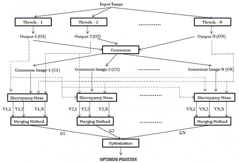
Figure 1. Flowchart of automatic reference image generation technique
Fernández-García et al. (2008) introduced a novel technique to automatically generate consensus ground truth for edge detector. However, it is a difficult task to apply the same approach to create consensus image for thresholding method, as both object and background pixels play an important role in binarization. Initially, the reference image is created by giving priority to object pixels as explained below. If $\left.\text { there are } N^{\prime} \text { (here } N=21\right)$ different algorithms for image thresholding $\left(O_{i}, i \in\{1,2 ;\right.$ $\cdots, N\}\}$ and $K^{\prime},$ ofthem are confirming apoinect then the output (Consersus, $\text { image }(C, i, j \in\{1,2, \cdots, N\}) \text { is assigned as object and vice-versa (See, Figure } 1)$$\text { Baddeley's discrepancy measurement } D \text { Baddeley ( } 1992)$ is used to compare each consensus image $C_{i}$ and $N$ different output images $O_{i}$ , to obtain comparison values $V_{i} \quad i=D\left(C_{i}, O_{i}\right) .$ The optimum vote or consensus level is chosen for ground truth image using two novel approaches namely: Minimean and Minimax.
2.1. Minimin method
The optimum consensus level can be determined by taking the minimum value of the mean of $j^{t h}(j \in\{1, \ldots, N\})$ level consensus and output of each of the methods (see, Figure 1).
$G_{j}=\frac{1}{N} \sum_{i=1}^{N} V_{j, i}$ (2)
Joptimum, min $\left(G_{j}\right) \in G_{j}$ (3)
2.2. Minimax method
The minimum value of the maximum of $j^{t h}$ consensus level $(j \in\{1, \ldots, N\})$ and output of each of the methods selects the optimum position for ground truth image (see Figure 1). Which can be expressed as follows:
$G_{j}=\max \left\{V_{j, i} | i \in\{1, \ldots, N\}\right\}$ (4)
$J_{\text {Optimum},} \max \left(G_{j}\right) \in G_{j}$ (5)
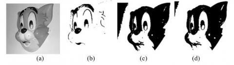
The reference image obtained by yielding priority to object pixel suffers from under segmentation (Minimean method) and over segmentation (Minimax method) as shown in Figure 2b and Figure 2c respectively. To counterbalance this error, the optimum consensus level is selected by taking the average of both the levels obtained from these methods (Minimean and Minimax). The proposed method not only improves the quality of ground truth image but also reduces the effect of noise as shown in Figure 3.
Figure 2. (a) original image of a mask and its reference image created via. (b) minimean method, (c) minimax method, & (d) average of minimean and minimax method
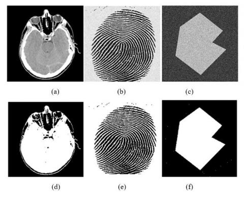
Figure 3. (a), (b), and (c) are standard original image of head CT, noisy finger print, and Noisy (Gaussian noise, Mean=0 Std.=50) septagon, while (d), (e) and (f) are their generated reference image via. consensus ground truth method
Although thresholding is a simple method of image binarization, it encounters difficulties when object and background distributions are overlapping leading to unimodal histogram. It is also difficult to locate threshold point in an image due to histogram stretching or equalization. Therefore to judge the efficacy of the thresholding methods, five different performance indices have been considered Sezgin and Sankur (2004) namely: F-measure (FM), modified Hausdorff distance (MHD), edge mismatch (EMM) error, relative area error (RAE) and object level consistency error (OCE) Polak et al. (2009). These metrics are normalized in such a way that their scores vary from 0 to1. Zero indicates correct classification and one implies the maximum error.
3.1. F-measure (FM)
This is a statistical measure to indicate the classification accuracy. It includes both precision and recall in its formulation as given below:
$F M=2 \times \frac{\text {Precision} . \text { Recall }}{\text { Precision }+\text {Recall}}$ (6)
Where, precision (see Eq.7) is the number of object pixels belonging to reference image and retained by the test image to the total number of relevant object pixels in both reference and test image and irrelevant object pixels in the test image. Recall (see Eq.8) is the ratio of number of relevant object pixels retained by test image to the total number of object pixels belonging to reference image.
Precission $=\frac{t p}{t p+f p}$ (7)
Recall $=\frac{t p}{t p+f n}$ (8)
The true positive (tp) is the number of pixels in the reference image corresponding to foreground and are detected as foreground. Similarly false positive $(f p)$ is the number of image points which are background but identified as foreground and false negative $(f n)$ is the cardinality of points that are foreground however detected as background in the binary (test) image.
3.2. Modified hausdorff distance (MHD)
The similarity in shape of the binarized region in both the thresholded (test) and reference image can be quantified using Hausdorff distance, which is defined as:
$H\left(F_{O}, F_{T}\right)=\max \left\{d_{H}\left(F_{O}, F_{T}\right), d_{H}\left(F_{T}, F_{O}\right)\right\}$ (9)
where, FT and FO are the foreground region in thresholded and ground truth image.
$d_{H}\left(F_{O}, F_{T}\right)=\max _{f_{O} \in F_{O}} d\left(f_{O}, F_{T}\right)=\max _{f_{O} \in F_{O}} \min _{f_{T} \in F_{T}}\left\|f_{O}-F_{T}\right\|$
and $\left\|f_{o}-F_{T}\right\|$ k represents the Euclidean distance between the two pixels of reference and thresholded objects.
The distance measure defined in Eq.9 suffers from lower discriminatory capability and lower sensitivity Sezgin and Sankur (2004). Hence, modified Hausdorff distance (MHD) is proposed in Sezgin and Sankur (2004) as:
$M D H\left(F_{O}, F_{T}\right)=\frac{1}{F_{O}} \sum_{f_{O} \in F_{O}} d\left(f_{O}, F_{T}\right)$ (10)
The modified Hausdorff distance is normalized between [0,1].
3.3. Edge mis-match error (EMM)
The Edge mismatch error (EMM) measure can be utilize to find the inaccuracy in fore-ground boundary on the binarized image Sezgin and Sankur (2004). This index is expressed as:
$E M M=1-\frac{C E}{C E+\omega\left[\sum_{k \in\{E O\}} \delta(k)+\alpha \sum_{k \in\{E O\}} \delta(k)\right]}$ (11)
With
$\delta(k)=\left\{\begin{array}{l}{\left|d_{k}\right|, i f\left|d_{k}\right|<\text {maxdist}} \\ {D_{\max } \quad, \text { Otherwise }}\end{array}\right.$
where,
CE=Number of common edge pixels between reference and thresholded image.
EO=Number of excess ground-truth edge pixels missing in the thresholded image.
ET=Set of excess thresholded edge pixels that are not found in reference image.
$\left|d_{k}\right|$=Euclidian distance of the kth excess edge pixel to a complementary edge pixel with in the search area determined by 'maxdist'.
If N is image dimension, then maxdist=0.025×N.
$\omega=\frac{10}{N},$ with $\alpha=2$
3.4. Relative area error (RAE)
This index compares the area between the segmented region in both ground-truth image and test image. It can be defined as:
$R A E=\left\{\begin{array}{l}{\frac{A_{O}-A_{T}}{A_{O}}, \text { if } A_{T}<A_{O}} \\ {\frac{A_{T}-A_{O}}{A_{T}}, \text { if } A_{T} \geq A_{O}}\end{array}\right.$ (12)
Where, A0 is the area of the reference image and AT is the area of thresholded image. A score of '0' indicates both images are similar, while '1' represents zero overlapping between the object area.
3.5. Object consistency error (OCE)
Object-level consistency error considers the size, shape and the position of each object for the performance evaluation of segmented images Polak et al. (2009). It quantifies the similarity (or discrepancy) between test and ground truth image at the object level. OCE has better discriminatory characteristics as it penalizes both the over and under segmentation.
Assume, $I_{O}=\left\{A_{1}, A_{2}\right\}$ is a ground truth with A1 and A2 as the object and background segmentation of 'I0'. Similarly test image $I_{T}=\left\{B_{1}, B_{2}\right\}$ contains B1 and B2 as object and background respectively. Then a partial error measure can be defined as:
$E_{O, T}\left(I_{O}, I_{T}\right)=\sum_{j=1}^{2}\left[1-\sum_{i=1}^{2} \frac{\left|A_{j} \cap B_{i}\right|}{\left|A_{j} \cap B_{j}\right|} \times W_{i, j}\right] W_{j}$
$W_{i, j}=\frac{1-\delta\left(\left|A_{j} \cap B_{i}\right|\right)\left|B_{i}\right|}{\sum_{k=1}^{2}\left(1-\delta\left(\left|A_{j} \cap B_{k}\right|\right)\right)\left|B_{k}\right|}$
$W_{j}=\frac{\left|A_{j}\right|}{\sum_{l=1}^{2}\left|A_{l}\right|}$ (13)
Where, $|\cdot|$ is the cardinality of the set, with $\delta(x)=\left\{\begin{array}{c}{1, \text { if } x=0} \\ {0, \text { Otherwise }}\end{array}\right.$
This partial error can be used to define OCE as:
$\operatorname{OCE}\left(I_{O}, I_{T}\right)=\min \left(E_{O, T}, E_{T, O}\right)$ (14)
Sezgin et al. Sezgin and Sankur (2004) suggests that some of these parameters are not independent, i.e. there is a certain amount of correlation between these measures. However the fact is not reported quantitatively. In this article Pearson correlation coefficient (PCC) Lee Rodgers and Nicewander (1988) is used to measure the amount of closeness between these indices. Table 2 represent the average value of PCC among these indices. It is clearly evident from the table that FM, MHD and EMM preserves distinct and non-redundant information. So, performance evaluation can be effectively done considering these three parameters only.
Table 2. Mean pearson correlation coefficient between different performance measures for DTU IMM face database Nordstom et al. (2004)
|
Different Parameters |
FM |
MHD |
EMM |
RAE |
OCE |
|
FM |
1 |
0.7855 |
0.4831 |
0.9937 |
0.8266 |
|
MHD |
0.7855 |
1 |
0.5574 |
0.8063 |
0.8497 |
|
EMM |
0.4831 |
0.5574 |
1 |
0.522 |
0.6035 |
|
RAE |
0.9937 |
0.8063 |
0.522 |
1 |
0.8487 |
|
OCE |
0.8266 |
0.8497 |
0.6053 |
0.8487 |
1 |
The performance indices FM, MHD and EMM provide different types of error for evaluation of thresholding methods and also normalized between 0 and 1. So an average of these metrics as shown in Eq.15, can be used as overall performance index.
$O P I=\frac{F M+M H D+E M M}{3}$ (15)
The overall performance index (OPI) is used to evaluate the performance of dif- ferent thresholding methods on six different databases containing more than 1800 images. These database include a wide variety of building Shao et al. (2003), texture Laws (1980), face Nordstom et al. (2004), iris CASIA (2004) and leaf images with varying illumination and background Weber (1999). A brief description of these databases are given in Table 3.
The value of OPI for different database is given in Table.4. From these results the following points can be observed:
All the image thresholding methods perform distinctively for different data- bases. Therefore no single algorithm can successfully segment the object from back- ground for all types of images.
The quality score for CalTech leave database Weber (1999) are close to 0 for most of the binary segmentation algorithms, which reveals the potentiality of these algorithms to segment single object images.
The efficiency of fuzzy logic Jawahar et al. (1997) and entropy based Sahoo et al. (1997), Sahoo and Arora (2006) thresholding methods are higher compared to other algorithms.
Table 3. Database specifications
|
Database |
Image Type |
Total Images |
Resolution |
Other Specifications |
|
Caltech Databases Weber (1999) |
Background |
452 |
378×251 |
Contains several objects with different background. |
|
Caltech Databases Weber (1999) |
Leaves |
186 |
896×592 |
3 leaves with different background |
|
CASIA Iris Database CASIA (2004) |
Iris Images |
753 |
640×400 |
It contains iris images of 100 pairs of twins |
|
DTU IMM Database Nordstom et al. (2004) |
Human Face |
240 |
640×480 |
7 Female and 33 male subjects without eye-glasses |
|
USC SIPI Database Laws (1980) |
Texture Images |
64 |
512×512 |
It contains monochrome texture images |
|
Zurich Database Shao et al. (2003) |
Building Images |
115 |
240×320 |
Different Building images |
This article also considers two important criteria to analyze the performance of consensus ground truth method such as:
(1) Accuracy: The reference image created using consensus of different thresholding methods must provide same ranking Fernández-García et al. (2008). Therefore to verify the robustness of this algorithm with varying number of thresholding methods, we carried out the following experiments:
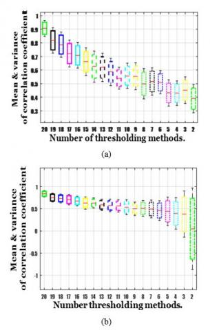
a. Figure 4a represents the mean and variance plot of correlation coefficient between the ranks of thresholding methods obtained with original reference image (considering 21 binarization techniques) and the reference image generated by random selection of thresholding method (Initially, we select 20 binarization methods and discard one algorithm in each step randomly to generate ground truth image.). Which illustrates the efficacy of consensus ground truth method with varying number of binarization techniques.
b. Similarly, the correlation coefficient between the ranks of different thresholding methods is calculated by discarding those methods which are not included in the training phase (see Figure 4b). As expected it preserves the robustness of consensus ground truth method up to certain level.
Table 4. Mean quality score of different thresholding methods for six different databases
|
Databases ⇉ Thresholding Methods |
Caltech Background |
Caltech Leaves |
CASIA Iris |
DTU IMM Face |
USC-SIPI Texture |
Zurich Building |
|
Convex Hull |
0.3933 |
0.4104 |
0.5145 |
0.5228 |
0.2964 |
0.3253 |
|
Histogram Aproximation |
0.4884 |
0.3373 |
0.4805 |
0.3785 |
0.5993 |
0.6103 |
|
Fuzzy Clustering |
0.2764 |
0.2329 |
0.3453 |
0.3568 |
0.2468 |
0.2178 |
|
Fuzzy Logic |
0.2383 |
0.2794 |
0.2654 |
0.3367 |
0.2369 |
0.1967 |
|
Iterative Threshold |
0.2406 |
0.2772 |
0.2681 |
0.3288 |
0.2244 |
0.2087 |
|
Kittler’s Minimum |
0.4881 |
0.3419 |
0.4834 |
0.3715 |
0.5974 |
0.6095 |
|
Otsu’s Inter class |
0.2454 |
0.2958 |
0.2644 |
0.3342 |
0.2502 |
0.2103 |
|
Moment Preserve |
0.2472 |
0.2369 |
0.3015 |
0.3197 |
0.2279 |
0.2437 |
|
Fuzzy compact |
0.3506 |
0.2517 |
0.4370 |
0.5448 |
0.2951 |
0.3385 |
|
Fuzziness Minimization |
0.3043 |
0.2886 |
0.3294 |
0.3424 |
0.2743 |
0.3292 |
|
Maximum Entropy |
0.2821 |
0.2315 |
0.3080 |
0.3486 |
0.2606 |
0.3018 |
|
Renyi’s Entropic |
0.2626 |
0.1985 |
0.2401 |
0.4637 |
0.2447 |
0.2989 |
|
Entropic Correlation |
0.2939 |
0.2436 |
0.2499 |
0.3244 |
0.2578 |
0.3571 |
|
Brink’s Cross-entropic |
0.3218 |
0.3334 |
0.3527 |
0.3163 |
0.3172 |
0.3139 |
|
Cross Entropic |
0.3054 |
0.3294 |
0.3325 |
0.3211 |
0.3066 |
0.3008 |
|
Tsalli’s Entropic |
0.2839 |
0.2178 |
0.2475 |
0.3376 |
0.2646 |
0.3312 |
|
Pal’s Local Entropic |
0.3264 |
0.2807 |
0.3574 |
0.3228 |
0.2513 |
0.3745 |
|
Renyi’s 2D Entropic |
0.3413 |
0.2539 |
0.3149 |
0.3445 |
0.2158 |
0.4033 |
|
Tsalli’s 2D Entropic |
0.3425 |
0.2482 |
0.3071 |
0.3103 |
0.2052 |
0.3920 |
|
Arimoto Entropic |
0.3564 |
0.2755 |
0.3331 |
0.4288 |
0.2187 |
0.4241 |
|
Iterative Partition |
0.2755 |
0.2199 |
0.4066 |
0.3976 |
0.2234 |
0.2296 |
The number of binarization methods required to generate reference image can not be changed after a certain level (Here, 3 methods can be discarded randomly to preserve $\approx 80 \%$ accuracy) to prevent inaccuracy in the performance. In addition the ground truth image, which is generated using consensus of some binarization algorithms can exclusively be used for the evaluation those methods only.
Figure 4. Mean and variance of correlation coefficient between the ranks of thresholding methods by (a) considering all the binarization methods & (b) discarding those methods, which aren’t participated in reference image creation
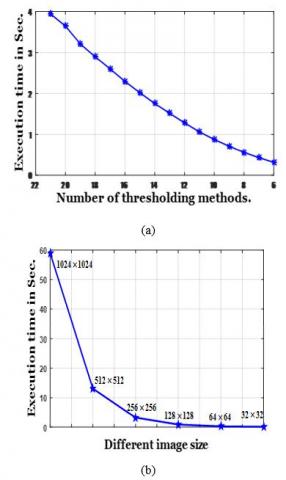
(2) Time Complexity: The Thresholding is used as a preprocessing step for many real time computer vision applications. Time required to decide the best binarization method is an important aspect for those applications. Figure 5a illustrates the time complexity of the consensus algorithm with varying number of binarization methods. It is clearly evident from this figure that minimum 3.2 seconds is required to generate consensus ground truth for maximum 80% accuracy. Similarly, Figure 5b represents the execution for different image size.
Figure 5. Execution time complexity of consensus ground truth method (a) with varying number of thresholding methods, and (b) for different size image
In this article we proposed a technique to automatically rank image thresholding methods, where the reference image is unavailable. The reference image is generated using consensus of different thresholding methods. The proposition is validates using 21 thresholding methods on six different database. The proposed averaging method for automatic selection of optimum consensus level ndot only eliminates the inaccuracy in over and under segmentation but also reduces the effect of noise. In prior art, the image data were mostly document image while present work includes a wide variety of building, texture, face, iris and leaf images with varying illumination and background. The performance of these methods are measured using a few indices as suggested by different literature. However, a quantitative analysis shows that only FM, MHD and EMM can well be used to serve the purpose. The overall performance is obtained as the average value of these indices. The numerical evidence of OPI indicates the best thresholding technique for particular type of images.
The authors would like to express their gratitude towards Prof. Prasanna K. Sahu, Department of Electrical Engineering, NIT, Rourkela-08, for his gracious encouragement and support throughout this work.
Albuquerque M., Esquef I. A., Mello A. R. G. (2004). Image thresholding using tsallis entropy. Pattern Recognition Letters, Vol. 25, No. 9, pp. 1059-1065. http://dx.doi.org/10.1016/j.patrec.2004.03.003
Baddeley A. (1992). An error metric for binary images. Robust Computer Vision: Quality of Vision Algorithms (S. R. E. K. Wichmann Verlag W. Fo¨rstner, Ed.), pp. 59-78.
Brink A. D., Pendock N. E. (1996). Minimum cross-entropy threshold selection. Pattern Recognition, Vol. 29, No. 1, pp. 179-188. http://dx.doi.org/10.1016/0031-3203(95)00066-6
Casia I. (2004). Chinese Academy of Sciences Institute of Automation. Casia Iris Image Database. http://english.ia.cas.cn/db/201610/t20161026_169399.html
Fernández-García N., Carmona-Poyato A., Medina-Carnicer R., Madrid-Cuevas F. (2008). Automatic generation of consensus ground truth for the comparison of edge detection techniques. Image and Vision Computing (Elsevier), Vol. 26, No. 4, pp. 496-511. http://dx.doi.org/10.1016/j.imavis.2007.06.009
Huang L. K., Wang M. J. J. (1995). Image thresholding by minimizing the measures of fuzziness. Pattern Recognition, Vol. 28, No. 1, pp. 41-51. http://dx.doi.org/10.1016/0031-3203(94)E0043-K
Jawahar C. V., Biswas P. K., Ray A. K. (1997). Investigations on fuzzy thresholding based on fuzzy clustering. Pattern Recognition, Vol. 30, No. 10, pp. 1605-1613. http://dx.doi.org/10.1016/S0031-3203(97)00004-6
Kapur J. N., Sahoo P. K., Wong A. K. C. (1985). A new method for gray-level picture thresholding using the entropy of the histogram. Computer Vision, Graphics, and Image Processing, Vol. 29, No. 3, pp. 273-285. http://dx.doi.org/10.1016/0734-189X(85)90125-2
Kittler J., Illingworth J. (1986). Minimum error thresholding. Pattern Recognition, Vol. 19, No. 1, pp. 41-47. http://dx.doi.org/10.1016/0031-3203(86)90030-0
Laws K. I. (1980). Uscipi report 940. Textured Image Segmentation. http://cdm15799.contentdm.oclc.org/cdm/ref/collection/p15799coll3/id/498876
Lee Rodgers J., Nicewander W. A. (1988). Thirteen ways to look at the correlation coefficient. The American Statistician, Vol. 42, No. 1, pp. 59-66. http://dx.doi.org/10.1080/00031305.1988.10475524
Li C. H., Lee C. K. (1993). Minimum cross entropy thresholding. Pattern Recognition, Vol. 26, No. 4, pp. 617-625. http://dx.doi.org/10.1016/0031-3203(93)90115-D
Liu Y., Li S. (2010). Two-dimensional arimoto entropy image thresholding based on ellipsoid region search strategy. In Multimedia Technology (ICMT), 2010 International Conference on, pp. 1-4. http://dx.doi.org/10.1109/ICMULT.2010.5631047
Marchitto A., Misale M. (2018). Experiments on parallel connected loops in single phase natural circulation: preliminary results. Mathematical Modelling of Engineering Problems, Vol. 5, No. 3, pp. 161-167. http://dx.doi.org/10.18280/mmep.050305
Nitrogiannis K., Gatos B., Pratikakis I. (2008). An objective evaluation methodology for document image binarization techniques. In 8th Iapr International Workshop on Document Analysis System (Das), pp. 217-224. http://dx.doi.org/10.1109/DAS.2008.41
Nordstom M. M., Larsen M., Sierakowski J., Stegmann M. B. (2004). The imm face database: An annotated dataset of 240 face images, informatics and mathematical modelling. Technical Univ. of Denmark, DTU, Denmark. http://www2. imm. dtu. dk/pubdb/p. php
Otsu N. (1975). A threshold selection method from gray-level histograms. Automatica, Vol. 11, No. 285-296, pp. 23-27. http://dx.doi.org/10.1109/TSMC.1979.4310076
Pal R. N., Pal S. K. (1989). Entropic thresholding. Signal Processing, Vol. 16, No. 2, pp. 97-108. http://dx.doi.org/10.1016/0165-1684(89)90090-X
Polak M., Zhang H., Pi M. (2009). An evaluation metric for image segmentation of multiple objects. Image and Vision Computing, Vol. 27, No. 8, pp. 1223-1227. http://dx.doi.org/10.1016/j.imavis.2008.09.008
Ramesh N., Yoo J. H., Sethi I. K. (1995). Thresholding based on histogram approximation. IEE Proceedings-Vision, Image and Signal Processing, Vol. 142, No. 5, pp. 271-279. http://dx.doi.org/10.1049/ip-vis:19952007
Ridler T. W., Calvard S. (1978). Picture thresholding using an iterative selection method. IEEE Transactions on Systems, Man and Cybernetics, Vol. 8, No. 8, pp. 630-632. http://dx.doi.org/10.1109/TSMC.1978.4310039
Rodríguez R. (2008). Binarization of medical images based on the recursive application of mean shift filtering: Another algorithm. Advances and Applications in Bioinformatics and Chemistry: AABC, Vol. 1, pp. 1.
Rodriguez R. (2010). A robust algorithm for binarization of objects. Latin Am. Appl. Res., Vol. 40.
Rosenfeld A. (1984). The fuzzy geometry of image subsets. Pattern Recognition Letters, Vol. 2, No. 5, pp. 311-317. http://dx.doi.org/10.1016/0167-8655(84)90018-7
Rosenfeld A., Torre P. D. L. (1983). Histogram concavity analysis as an aid in threshold selection. Systems, Man and Cybernetics, IEEE Transactions on, No. 2, pp. 231-235. http://dx.doi.org/10.1109/TSMC.1983.6313118
Sahoo P. K., Arora G. (2006). Image thresholding using two-dimensional tsallis–havrda–charvát entropy. Pattern Recognition Letters, Vol. 27, No. 6, pp. 520-528. http://dx.doi.org/10.1016/j.patrec.2005.09.017
Sahoo P. K., Soltani S., Wong A. K. C., Chen Y. (1988). A survey of thresholding techniques. Computer Vision, Graphics, and Image Processing (Elsevier), Vol. 41, No. 2, pp. 233-260. http://dx.doi.org/10.1016/0734-189X(88)90022-9
Sahoo P. K., Wilkins C., Yeager J. (1997). Threshold selection using renyi’s entropy. Pattern Recognition, Vol. 30, No. 1, pp. 71-84. http://dx.doi.org/10.1016/S0031-3203(96)00065-9
Sahoo P., Arora G. (2004). A thresholding method based on two-dimensional renyi’s entropy. Pattern Recognition, Vol. 37, No. 6, pp. 1149-1161. http://dx.doi.org/10.1016/j.patcog.2003.10.008
Sezgin M., Sankur B. (2004). Survey over image thresholding techniques and quantitative performance evaluation. Journal of Electronic Imaging, Vol. 13, No. 1, pp. 146-168. http://dx.doi.org/10.1117/1.1631315
Shaikh S. H., Maiti A. K., Chaki N. (2013). A new image binarization method using iterative partitioning. Machine Vision and Applications, Vol. 24, No. 2, pp. 337-350. http://dx.doi.org/10.1007/s00138-011-0402-4
Shao H., Svoboda T., Gool L. V. (2003). Zubud-zurich buildings database for image based recognition. Computer Vision Lab, Swiss Federal Institute of Technology, Switzerland. Zurich, Switzerland. http://www.vision.ee.ethz.ch/showroom/
Smith E. H. B. (2010). An analysis of binarization ground truthing. In 9th Iapr International Workshop on Document Analysis System (Das). http://dx.doi.org/10.1145/1815330.1815334
Stathis P., Kavallieratou E., Papamarkos N. (2008). An evaluation technique for binarization algorithms. J. Univ. Comput. Sci., Vol. 14, No 18, pp. 3011–3030. https://doi.org/10.3217/jucs-014-18-3011
Tsai W. H. (1985). Moment-preserving thresolding: A new approach. Computer Vision, Graphics, and Image Processing, Vol. 29, No. 3, pp. 377-393. http://dx.doi.org/10.1016/0734-189X(85)90133-1
Weber M. (1999). Leaves Dataset, California Institute of Technology. http://www.vision.caltech.edu/archive.html
Yen J. C., Chang F. J., Chang S. (1995). A new criterion for automatic multilevel thresholding. Image Processing, IEEE Transactions on, Vol. 4, No. 3, pp. 370-378. http://dx.doi.org/10.1109/83.366472