J. Gold Beulah Patturose* | R. Priscilla
© 2026 The authors. This article is published by IIETA and is licensed under the CC BY 4.0 license (http://creativecommons.org/licenses/by/4.0/).
OPEN ACCESS
In this article, brain magnetic resonance imaging (MRI) is classified into healthy and cancer images, and then the cancer region is segmented. The segmented cancer region from the brain MRI is compressed using a lossless compression technique, and the compressed segmented cancer region is transmitted through an additive white gaussian noise (AWGN) wireless channel by the wireless transmission system. This transmission section consists of a noise reduction filter, a multi-resolution transform module, a multi-level feature computation module, and a classification module with a segmentation algorithm. The noise in the acquired brain MRI is detected and suppressed using the weighted adaptive median filter (WAMF). The low- and high-frequency components from this noise-suppressed image are separated by passing the image through the non-subsampled contourlet transform (NSCT) module, which acts as the multi-resolution module. The multi-level features Local Binary Pattern (LBP) and Local Ternary Pattern (LTP) are computed from these NSCT sub-bands, and then they are classified using the proposed multi-level featured convolutional neural networks (MLF-CNN) classification architecture. The segmentation module segments the cancer regions from the entire cancer case image, and the cancer region alone is compressed using a lossless compression method. The compressed patterns are transmitted through the wireless transmission system. The proposed method reaches 98.69% Segmentation Sensitivity (SSe), 98.67% Segmentation Specificity (SSp), and 98.63% Segmentation Accuracy (SA) on the brain images in Kaggle dataset. The proposed method reaches 98.61% SSe, 98.7% SSp, and 98.77% SA on the brain images in the Jun Cheng dataset. The results show that the proposed framework stated in this article segments the tumor regions in the brain MRI correctly. Further, the performance of the wireless communication-based transmission and reception system has been analyzed using Bit Error Rate (BER) and Eb/N0.
image, lossless, compression, transformation, encoding, cancer, features
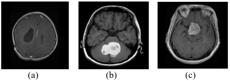
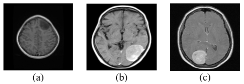
The brain is an important organ in the human body that controls all the active movements of various organs, and its functions are monitored. The cells in the human brain grow linearly, and sometimes cell growth is affected due to various reasons such as genetics, food habits, and medications [1, 2]. Due to this, the cells in the human brain are abnormally developed, which leads to malignancy. In the current worldwide scenario, the influence of malignancy is strong, as per the World Health Organization report 2023. Brain tumors affect all kinds of people around the world irrespective of gender. Though a large number of brain tumors are identified by physicians and radiologists, three important brain cancers are glioma, meningioma, and pituitary [3]. The glioma tumor is identified as a spinal cord tumor that severely causes headache, nausea, and vomiting. The primary solution to this tumor is surgery or chemotherapy with radiation treatment. The survival rate of the patient in this tumor category depends entirely on the age of the patient, location, and size of the tumors in the brain region. The five-year average survival rate in this category is less than 18% [4]. Meningioma tumors start on the membranes of the brain and spread into the spinal cord. The meningioma is categorized into three grades. Based on the meningioma tumor grades, the severity levels vary. The meningioma tumor with grade 1 has a higher survival rate; the meningioma tumor with grade 2 has approximately a 53% survival rate under proper medical treatment, and the meningioma tumor with grade 2 have less than a 2-year survival rate. Pituitary tumors are formed in the pituitary gland, which is located at the bottom of the brain [5, 6]. Hormonal imbalance in the pituitary gland is the main cause of pituitary tumors. The non-carcinoma pituitary tumor survival rate is 100% with proper treatment, and the carcinoma pituitary tumor survival rate is about 71%. The lifespan and survival rate of the affected patient are based on the tumor type, treatment procedures, and patient age. All three types of brain tumors are screened using Computed Tomography (CT) and MRI technology [7]. Clear visualization of the internal regions is possible in MRI. Hence, MRI brain imaging is used in this research work to detect any abnormality in the human brain. Figure 1(a) shows a glioma MRI, Figure 1(b) shows a carcinoma case of meningioma MRI, and Figure 1(c) shows a carcinoma pituitary case MRI.
Due to the bandwidth limitation of the wireless channel, the images should be compressed before they are processed into the channel [8]. In this research work, a lossless compression technique has been used for medical image transmission and reception, where the loss of pixels leads to false decisions. The brain tumor-detected images are transmitted through the wireless channel to the remote receiver. Due to the presence of noise and other interference in the wireless channel, the received images are affected. Hence, the analysis of wireless channels with respect to various modulation techniques and Bit Error Rate (BER) is important [9, 10]. This research work analyzes the impact of wireless channel interference on the received images in the wireless reception system.
The primary objective of this research article is to construct an integrated model for MRI image classification, tumor localization, compression of the tumor regions, and wireless transmission of diagnostically relevant brain MRI information. The proposed MLF-CNN is a key technical component within this framework and is specifically designed to improve the classification of healthy and cancerous brain MRI images by exploiting multi-level texture information extracted from NSCT sub-bands using LBP and LTP descriptors.
The relationship among the individual modules has now been clarified in the revised manuscript. The modules in the proposed system are not independent contributions; rather, they form a sequential processing pipeline in which the output of one stage serves as the input to the subsequent stage. In particular, the classification stage identifies cancerous MRI images, the segmentation stage extracts only the diagnostically relevant tumor region, and the compression stage reduces the transmission data volume while preserving the information through lossless compression. The resulting compressed tumor information is then transmitted through the wireless channel.
The effective and dependable transmission of diagnostically significant brain MRI data over a noisy wireless communication channel while reducing needless transmission of irrelevant image regions is, thus, the main research issue addressed in this study. The main deep learning contribution that makes it possible to accurately identify malignant MRI images prior to the segmentation and transmission processes is the MLF-CNN.
The entire paper is sub-sectioned, where the state-of-the-art methods in the brain tumor detection process and wireless communication system are depicted in Section 2, the proposed brain tumor detection method with its wireless channel transmission and reception are given in Section 3, the results of this method are highlighted in Section 4, and the conclusion along with future works are given in Section 5.
Asif et al. [10] developed an ensemble training workflow methodology for detecting and locating the non-linear tumor pixels in the brain MRI. This work combined the dependency-based Inception and Xception models with the proposed tumor detection methods to improve the tumor localization accuracy. Based on the training values, the validation accuracy was improved to 96% on open-access brain imaging datasets. The model was cross-validated through different statistical and chi-square tests to obtain the optimum tumor segmentation results. This work obtained 97.16% Segmentation Sensitivity (SSe), 97.43% Segmentation Specificity (SSp), and 97.10% Segmentation Accuracy (SA) for the brain cancer images in the Kaggle dataset and also obtained 97.98% SSe, 97.15% SSp, and 97.65% SA for the brain cancer images in the Jun Cheng dataset. Ahmed et al. [11] devised a brain tumor detection system using a hybrid learning technique, which combined the Vision Transformer Model (VTM) and the Gated Recurrent Unit (GRU). The entire brain MRI was divided into a number of patches with their corresponding generated header and these patches were fed into the VTM model with the implementation of GRU module in this classification framework to obtain higher brain image classification results. This work was tested by three radiologists to perform validation on the obtained experimental results. This methodology obtained 96.12% SSe, 97.28% SSp, and 97.65% SA for the brain cancer images in the Kaggle dataset and obtained 97.17% SSe, 97.96% SSp, and 97.67% SA for the brain cancer images in Jun Cheng dataset. Rao et al. [12] used ResNet50 classification model to differentiate brain cancer MRI from non-brain cancer MRI by implementing the non-linear projection-modeling framework. This methodology used a systematic combination of the ResNet features and the projection directions to increase the final brain cancer MRI detection accuracy through the data augmentation process. Higher performance efficiency was obtained in this work by testing this proposed system with other deep learning models. The authors obtained 96.09% SSe, 96.96% SSp, and 96.56% SA for the brain cancer images in the Kaggle dataset and obtained 96.87% SSe, 96.45% SSp and 96.92% SA for the brain cancer images in Jun Cheng dataset.
Abdusalomov et al. [13] utilized YOLO-v7 algorithm for performing pre-training on large brain imaging datasets. The fine-tuning of this transfer algorithm was performed through the learning process in this work. Three types of brain tumors were identified and tumor regions in these images were segmented with the UNet algorithm with fine-tuning hyper parameters on this designed architecture. The investigations of this proposed model were performed on high configured processor to increase the detection speed of the entire system. This method obtained 95.38% SSe, 95.28% SSp and 95.29% SA for the brain cancer images in the Kaggle dataset and obtained 95.67% SSe, 95.87% SSp and 95.76% SA for the brain cancer images in the Jun Cheng dataset.
Khairandish et al. [14] combined Convolutional Neural Networks (CNN) methodology and multi-kernel polynomial-based Support Vector Machine (SVM) classifier to form the hybrid algorithm to detect the tumor brain MRI. The threshold technique was implemented on these images to segregate the tumor regions from the healthy pixel regions in the brain images. The authors obtained 94.87% SSe, 94.98% SSp and 94.97% SA for the brain cancer images in the Kaggle dataset and obtained 95.18% SSe, 94.15% SSp, and 94.13% SA for the brain cancer images in the Jun Cheng dataset. Zhang et al. [15] used a skip connection method for the brain tumor detection process using the U-Net segmentation framework. The Attention Gate Residual (AGR) model was used in this work to develop the learning parameters of this classification model for improving the brain tumor detection rate. The attention gates in this proposed architecture were pre-trained the entire dataset of images to obtain higher classification results on different imaging datasets. This work was significantly evaluated on different platforms to validate the results. This work obtained 94.17% SSe, 94.65% SSp, and 93.28% SA for the brain cancer images in the Kaggle dataset and obtained 94.76% SSe, 93.87% SSp, and 93.76% SA for the brain cancer images in the Jun Cheng dataset.
Vikraman and Afthab [16] proposed an autoencoder-based image compression method for brain MRI images. This method combined the Discrete Cosine Transform (DCT) and the encoding technique to compress the pixels in the brain images. Seenuvasamurthi et al. [17] used deep learning concepts to compress the brain MRI images. In this work, a deep neural network algorithm was used to compress the group of pixels, and the compressed images were transmitted and reconstructed at the receiver side.
The novelties of this research article have been determined by analyzing the above conventional methods, and they are stated below.
•In previous methods, either internally derived features (through convolution layers of CNN) or externally derived features (through algorithms based on patterns, shapes, and sizes) are used for the brain tumor detection process. In this research work, both internally and externally derived features are used for the brain tumor detection process to improve the tumor detection rate.
•The layers of the proposed MLF-CNN have been constructed in parallel with more convolutional layers to produce higher-order features, which increases the tumor image detection rate.
In this proposed work, the NSCT module has been combined with the multi-level feature extraction module to improve the performance of the entire classification system. By using NSCT to give a multi-resolution and directional representation of the MRI image, it is possible to assess the structural information at various frequency levels without losing spatial information due to downsampling. In order to provide comparable local texture descriptions from the NSCT sub-bands, LBP and LTP are integrated. Local intensity patterns can be well represented by LBP, while LTP offers a three-level encoding technique that is more resilient to noise and slight intensity fluctuations. Therefore, rather than depending just on raw-image features or a single constructed descriptor, their combined use is meant to provide richer texture information. Instead of relying solely on traditional CNN features that were taken straight from the original MRI image, the suggested MLF-CNN is then made to train discriminative representations from these multi-level features.
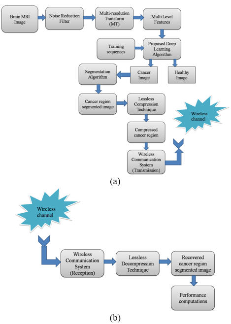
In this article, the brain MRI image is classified into healthy and cancer image and then the cancer region is segmented. The segmented cancer region from the brain MRI is compressed using a lossless compression technique, and the compressed segmented cancer region is transmitted through the wireless AWGN channel by the wireless transmission system. The entire medical image compression-based wireless transmission system is illustrated in Figure 2(a). This transmission section consists of a noise reduction filter, a multi-resolution transform module, a multi-level feature computation module, and a classification module with a segmentation algorithm. The noise in the acquired brain MRI is detected and suppressed using WAMF. The low- and high-frequency components from this noise-suppressed image are separated by passing the image through the NSCT module, which acts as the multi-resolution module. The multi-level features are computed from these NSCT sub-bands, and then they are classified using the proposed MLF-CNN classification architecture. The segmentation module segments the cancer regions from the entire cancer case image, and the cancer region alone is compressed using a lossless compression method. The compressed patterns are transmitted through the wireless transmission system. Figure 2(b) shows the wireless image reception system, which performs the reverse operation of the transmission module. The received cancer region from the wireless channel is decompressed and recovered at the wireless reception system.
Figure 2. Image transmission and reception model, (a) semantic wireless image transmission system using a deep learning algorithm, and (b) semantic wireless image reception system
3.1 Preprocessing
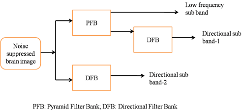
This stage consists of a noise reduction filter, a multi-resolution transform module, multi-level feature computation module. The noises in the acquired brain MRI are detected and suppressed using WAMF. The noise-suppressed brain MRI is further decomposed into low-frequency subbands and directional subbands using the NSCT approach, which is depicted in Figure 3.
Figure 3. Non-subsampled contourlet transform (NSCT) structure with pyramidal and directional filter banks (DFB)
The NSCT transformation process is used to decompose the entire image into multiple sub-bands with different frequency ranges. This helps to compute the external features from the image to differentiate the objects in the image. Many researchers have used the Contourlet transformation approach for the decomposition process. The shift-invariant property of this transform is poor, which generates errors during the transformation process. In order to improve the shift-invariant property of each pixel in the image, NSCT has been used in this article. This transform has been applied with respect to different scales and directions to improve the shift-invariant property of the pixels. Due to this shift-invariant property, the artifacts are mitigated during the decomposition process. Due to its multi-scale and multi-directional property, the edge pixels in the image during the decomposition process are preserved.
The NSCT can function at different scales with respect to different directional and pyramidal properties. It is designed with directional filter banks (DFB) and a pyramidal filter bank (PFB), which exhibit the shift-invariant property. The PFB is designed by implementing two-channel dimensional filter banks. This filter bank is constructed with a low-pass filter and a high-pass filter. The noise spectrum from the image has been eliminated by passing the image through this PFB. The DFB is designed using a two-channel fan filter, which splits the image into directional wedges.
As illustrated in Figure 3, the noise-suppressed brain MRI image is passed through the PFB and DFB. The PFB decomposes the image and produces the low-frequency subband and high-frequency subband. This high-frequency subband is further passed through the DFB to produce the directional subband-1, and the DFB in the low part of this structure produces the directional subband-2. The decomposed sub-bands from the noise-suppressed brain image are combined into NSCT Feature Matrix (NFM) which is fed into the proposed classifier.
3.2 Multi-level features
The features are correlated with the final brain image classification rate and hence it plays a important role in the classification process of the entire system. In this article, the multi-level features are used to compute the multi-variations of each pixel with respect to its surrounding pixels and the computed multi-level features are fed into the proposed classifier to perform the classification process. The LBP and LTP are used as the multi-level features, and they are explained in the following steps.
|
Algorithm 1: Local Binary Pattern and Local Ternary Pattern feature computation process |
|
Input: Two dimensional NFM; Outputs: LBP and LTP features;
Start; To compute the LTP feature, the following steps are followed. Step 1: The 3 × 3 window is placed at the initial position of the pixel (center place) over two dimensional NFM. Step 2: The intensity value of the surrounding pixel over the intensity value of the center pixel is absolute subtracted and if the subtracted value is negative, then replace the intensity value of the surrounding pixel into ‘0’ else replace the intensity value of the surrounding pixel into ‘1’. Step 3: Perform step 2 for all the surrounding pixel with respect to the center pixel. After step 3, all the surrounding pixel value is either ‘0’ or ‘1’. Step 4: All the surrounding eight binary values are now converted into decimal value which represents the computed feature value of the center pixel. Step 5: Move the window to next pixel position and perform step 2 to step 4 until there is no more pixel in two dimensional NFM, the final value is called as LBP. To compute the LTP feature, the following steps are followed. Step 6: If the intensity value of each surrounding pixel(gi) is greater than gc + p, then surrounding pixel value is set to +1. If gi-gc < p, then the surrounding pixel is set to 0. If gi $\leq$ gc-p, then -1 is set in the place of surrounding pixel. Step 7: The new window1 is constructed by changing the value -1 to 0 and the surrounding eight binary valuesare converted into decimal value which is representing LTP feature 1. Step 8: The new window 2 is constructed by changing -1 to +1 and +1 to 0 and the surrounding eight binary values is converted into decimal value which is representing LTP feature 2. Step 9: Move the window to next pixel position and perform step 6 to step 8 until there is no more pixel in the two-dimensional NFM, the final value is called as LTP1 and LTP feature images. End; |
The computed multi-level features are now combined into a two-dimensional Feature Correlating Matrix (FCM) and this is fed into the proposed classifier to perform the classification process for the brain tumor detection system.
3.3 Brain image classification
Brain image classification is the process of differentiating brain images into either a tumor case or a non-tumor case based on the external features, which are generated through the feature computational process. Though numerous brain tumor detection and classification systems use deep learning algorithms in conventional methods, the overfitting problem occurs, and the final brain imaging classification rate is reduced due to this overfitting issue. These conventional limitations are overcome by proposing a novel CNN architecture for performing the brain image classification process. This proposed classification CNN architecture receives the FCM from the feature computation, and based on the training levels, the final brain image classification results are produced.
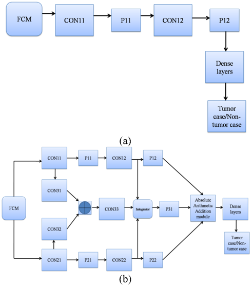
The MLF-CNN architecture is proposed in this paper for performing the brain MRI image classification process. The fundamental structure of this proposed MLF-CNN is derived from the conventional LeNet CNN architecture, which is illustrated in Figure 4(a). This LeNet CNN architecture contains two Convolutional layers and two pooling layers, with three dense layers to produce the brain MRI classification results. The FCM, which is computed from the feature computation process, is fed into the first Con11, which is constructed and designed with 32 kernels. Each kernel performs the convolution process between the FCM and its kernel value using a linear convolution process to produce the first layer features. This feature is size reduced by passing them through the Max-pool layer of P1. This output is transferred through the second CON12, which is constructed and designed with 32 kernels.
Each kernel in this CON12 performs the convolution process between the P1 output and its kernel value using a linear convolution process to produce the second layer features. This feature is size-reduced by passing them through the Max-pool layer of P2. The feature output from P2 is fed into three dense layers (4096 neurons in the first layer, 4096 neurons in the second layer, and 512 neurons in the third layer) which forwards the generated second layer features by multiplying the feature value with the weights of the neurons in each internal layer. The summation of all the feature values in the third dense layer produces the tumor case or non-tumor case results.
This conventional LeNet CNN architecture uses two layer features to produce the tumor or non-tumor case results. Though this architecture level and its process are simple, its final classification rate is low due to the generation of low-level and lower-order layer features by this architecture. This limitation has been overcome by proposing the MLF-CNN architecture for the effective classification of the brain MRI images in this paper. This proposed MLF-CNN contains seven Convolutional layers, five pooling layers, and three dense layers as illustrated in Figure 4(b). By including a larger number of convolutional layers in the conventional LeNet CNN architecture, this proposed MLF-CNN architecture is able to produce a larger number of internal features. Through the generation of a large number of internal features, the final brain imaging classification rate is improved than the conventional architecture.
The convolutional layers of this proposed MLF-CNN architecture are given in the following Eqs. (1)–(8).
Convolutionallayers$=\{$ CON11, CON12, CON21, CON22, CON31, CON32, CON33$\}$ (1)
CON11— —→32 filters with $3 \times 3$ kernel filter (2)
CON21— —→64 filters with $5 \times 5$ kernel filter (3)
CON21— —→32 filters with $7 \times 7$ kernel filter (4)
CON22— —→64 filters with $7 \times 7$ kernel filter (5)
CON31— —→512 filters with $5 \times 5$ kernel filter (6)
CON32— —→256 filters with $3 \times 3$ kernel filter (7)
CON33— —→512 filters with $7 \times 7$ kernel filter (8)
The pooling layers of this proposed MLF-CNN architecture are given in the following Eq. (9).
Poolinglayers$=\{P 11, P 12, P 21, P 22, P 33\}$ (9)
The FCM, which is computed from the feature computational process, is fed into the first Con11, which is constructed and designed with 32 kernels and a size of 3 × 3 (upper part of the proposed MLF-CNN architecture). Each kernel performs the convolution process between the FCM and its kernel value using a linear convolution process to produce the features. This feature is size reduced by passing them through the Max-pool layer of P11. This output is transferred through the second CON12 which is constructed and designed with 64 kernels and a size of 5 × 5. This feature is size reduced by passing them through the Max-pool layer of P21.
Similarly, the FCM is fed into first Con11 which is constructed and designed with 32 kernels and size of 7 × 7 (lower part of the proposed MLF-CNN architecture). Each kernel performs the convolution process between the FCM and its kernel value using linear convolution process to produce the features. This feature is size reduced by passing them through the Max-pool layer of P21. This output is transferred through the second CON22 which is constructed and designed with 64 kernels and a size of 7 × 7. This feature is size-reduced by passing it through the Max-pool layer of P22.
The CON11 and CON21 output sequences are passed through the Convolutional layers that are present in the middle part of the proposed MLF-CNN architecture CON31 and CON32, respectively. CON31 is configured by 512 filters and a size of 5 × 5 and CON32 is configured by 256 filters and a size of 3 × 3. The outputs from both CON32 and CON31 are now added and the added sequences are fed into CON33 which is constructed and designed with 512 kernels and size of 7 × 7. Now, the integration process is applied between the output sequences of CON12, CON22 and CON33 by the integrator as depicted in the following Eq. (10).
Integrator$=\{$CON12 output, CON22 output, Con33 coutput$\}$ (10)
The integrated sequences are now size reduced by passing them through P33. The output sequences of P21, P22 and P33 are now added by Absolute Arithmetic Adder (AAA) module and its added sequences are fed into dense layers (2048 neurons in the first layer, 512 neurons in the second layer and 2 neurons in the third layer), which forward the generated features by multiplying the feature value with the weights of the neurons in each internal layer. The summation of all the feature values in the third dense layer produces the tumor case or non-tumor case results.
This proposed MLF-CNN architecture has been optimized by proper hyperparameter selection and its application to the design. The number of iterations of the training set is defined as BGYepochs, and this design is set to a 150-epoch count. By increasing the epoch count of the optimization, the final classification rate will increase. This proposed architecture tuned by 12,456,000 parameters using the Adam optimization process. The dropout is 0.2, which is overcome by implementing SoftMax at the end of the dense layers. The Sigmoid Activation function has been used, and zero weight decay is used in this design to get the desirable classification results.
Figures 5(a)-(c) shows the classification results of the proposed MLF-CNN architecture on the Kaggle dataset with respect to glioma case, meningioma case and pituitary case.
Figure 5. Classification results of the proposed multi-level featured convolutional neural networks (MLF-CNN) architecture on the Kaggle dataset, (a) Glioma case, (b) meningioma case, and (c) pituitary case
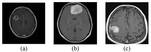
Figures 6(a)-(c) shows the classification results of the proposed MLF-CNN architecture on Jun Cheng dataset with respect to glioma case, meningioma case and pituitary case.
Figure 6. Classification results of the proposed multi-level featured convolutional neural networks (MLF-CNN) architecture on Jun Cheng dataset: (a) glioma case (b) meningioma case and (c) pituitary case
Table 1. Hyperparameters illustrating the proposed multi-level featured convolutional neural networks (MLF-CNN) architecture
|
Hyper Parameters |
Specific Values |
|
Batch size |
50 |
|
Learning rate |
0.001 |
|
Loss function |
Binary Cross entropy |
|
Optimizer |
Adam |
|
Data augmentation methods |
Left and Right |
|
Epochs |
120 |
|
Activation function |
ReLU |
For the reproduction of the proposed MLF-CNN architecture, the hyper parameters of the proposed design have been given in Table 1.
The cancer region should be segmented from the entire cancer case image in order to take the further medication for expanding the life span of the patient. In this article, the following steps are used to segment the cancer region in the cancer case image.
|
Cancer Region Segmentation Algorithm |
|
Input: Cancer case classified brain MRI; Output: Cancer region segmented image; Start; Step 1: The pixels in the cancer case classified brain MRI are expanded in its boundary with the radius of 0.3mm using ‘dilation’ process. Step 2: The pixels in the cancer case classified brain MRI are shrunk in its boundary with the radius of 0.2mm using ‘erosion’ process. Step 3: The image in step 2 is subtracted from the image obtained from step 1 to locate the cancer pixels. Step 4: The cancer like false pixels is removed using connected component algorithm. In this article, 4-pixel connected component algorithm is used. End; |
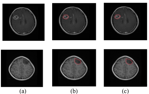
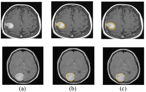
Figure 7(a) shows the glioma source brain MRI (Column-1), Figure 7(b) shows the segmentation outputs by manual process (Column-2), and Figure 7(c) shows the segmentation output by the proposed MLF-CNN method in this paper (Column-3).
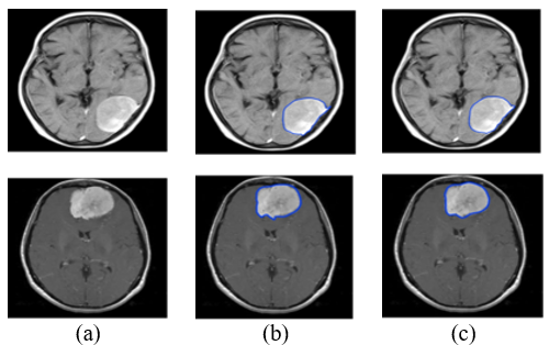
Figure 8(a) shows the MENINGIOMA source brain MRI (Column-1), Figure 8(b) shows the segmentation outputs by manual process (Column-2), and Figure 8(c) shows the segmentation output by the proposed MLF-CNN method in this paper (Column-3).
Figure 7. Glioma tumor segmentation results, (a) brain magnetic resonance imaging (MRI), (b) segmentation by manual, and (c) segmentation by proposed multi-level featured convolutional neural networks (MLF-CNN)
Figure 8. Meningioma tumor segmentation results, (a) brain magnetic resonance imaging (MRI), (b) segmentation by manual, and (c) segmentation by proposed multi-level featured convolutional neural networks (MLF-CNN)
Figure 9. Pituitary tumor segmentation results, (a) brain magnetic resonance imaging (MRI), (b) segmentation by manual, and (c) segmentation by proposed multi-level featured convolutional neural networks (MLF-CNN)
Figure 9(a) shows the Pituitary source brain MRI (Column-1), Figure 9(b) shows the segmentation outputs by manual process (Column-2), and Figure 9(c) shows the segmentation output by the proposed MLF-CNN method in this paper (Column-3).
The loss of bits in the transmitted medical image is very important for diagnosing cancer severity in remote telemedicine mode. Therefore, the cancer segmented brain MRI is compressed by Lempel-Ziv-Welch (LZW) compression technique in this research work. It is a lossless image compression method, which is applied to the entire cancer-segmented image to produce the compressed image. This LZW compressed image is transmitted to the wireless channel through the wireless transmission system.
3.4 Wireless transmission and reception system
Error detection and correction are important for obtaining the error-free transmitted cancer region segmented image at the receiver [9]. Hence, Forward Error Correction (FEC) is employed in this work to mitigate the errors in the received image. In this paper, a Convolutional Encoder/ Decoder is used as the FEC technique to mitigate the errors in both transmitted and received images. The compressed image is transmitted to the receiver through the wireless channel. In this article, an AWGN channel is used between the transmitter and receiver. This channel adds white Gaussian noise to the transmitted pixels in the simulation medium. The zero-mean distributed noise is added in this channel, and it has a uniform power spectral density for all set of frequencies [10].
The convolutional encoder is designed using shift registers and a modulo-2 arithmetic adder (XOR). It encodes the incoming bits into the transmitted data by including redundancy bits. The code rate and the constraint length are the important parameters to design the convolutional encoder. The code rate is designed as the ratio of the input bits to the output bits. The desired code rate is directly proportional to the throughput of the output patterns. The constraint length represents the current output bits with respect to the input bits. The constraint length is inversely proportional to the error rate. Based on the code rate and the constraint length, the number of shift registers is selected. In this article, Quadrature Phase Shift Keying (QPSK) modulation is used as the digital modulation technique, and the code rate of the convolutional encoder is set to 0.5, where the number of input bits is 2048 and the number of output bits is 4096, as illustrated in Table 2.
Table 2. Encoder/decoder design specifications
|
Design Parameters |
Assigned Values |
|
Encoder/Decoder |
Convolutional code |
|
Number of input bits |
2048 |
|
Number of code word bits (output) |
4096 |
|
Code rate |
0.5 |
|
Modulation type |
QPSK |
|
Wireless channel type |
AWGN |
This research work uses two types of brain MRI imaging datasets, Kaggle and Jun Cheng. Both datasets contain different numbers of brain MRI images with ground-truth annotated images [18, 19].
The Kaggle dataset [20] contains 1200 brain MRI images, and these images are typed into tumor cases and non-tumor cases. The tumor case contains 750 brain MRI images, and the non-tumor case contains 450 brain MRI images. The size of the images in this dataset is about 512 × 512 pixels. The tumor case brain MRI images are further typed into glioma, meningioma, and pituitary. All these brain images in this dataset are validated by a neurologist and cross-verified by two independent physicians. From this dataset, 60% of brain MRI images are trained, and the remaining 40% of brain MRI images are tested. Hence, 450 tumor case brain images are trained, and the remaining 300 tumor case brain images are tested. Hence, 270 non-tumor case brain images are trained and the remaining 180 non-tumor case brain images are tested. The proposed system correctly identifies 294 tumor case brain images over 300 tumor case brain images and hence, the classification accuracy is about 98% for tumor case. The proposed system correctly identifies 176 non-tumor case brain images over 180 non-tumor case brain images and hence the classification accuracy is about 97.7% for non-tumor cases for the Kaggle dataset.
The scientist Jun Cheng constructed the Jun Cheng dataset [21], and further, this dataset was maintained by the Cancer Agency Research Center, China. This dataset contains 6500 brain MRI images, and these images are divided into tumor cases and non-tumor cases. The tumor case contains 3250 brain MRI images, and the non-tumor case contains 3250 brain MRI images. The size of the images in this dataset is about 512 × 512 pixels. The tumor case brain MRI images are further typed into glioma, meningioma, and pituitary. All these brain images in this dataset are validated by a neurologist and cross-verified by two independent physicians. From this dataset, 60% of brain MRI images are used for training, and the remaining 40% of brain MRI images are tested. Hence, 1950 tumor case brain images are trained, and the remaining 1300 tumor case brain images are tested. Hence, 1950 non- tumor case brain images are trained, and the remaining 1300 non- tumor case brain images are tested.
The proposed system correctly identifies 1286 tumor case brain images over 1300 tumor case brain images, and hence the classification accuracy is about 98.9% for tumor case. The proposed system correctly identifies 1285 non-tumor case brain images over 1300 non-tumor case brain images and hence the classification accuracy is about 98.8% for non-tumor case in the Jun Cheng dataset.
To reduce the risk of data leaking, the dataset was split into 60% training and 40% testing subsets using a random splitting process carried out at the patient level instead of the individual image level. As a result, the training and testing subsets did not contain brain MRI images from the same patient. Between the two subsets, the class distribution was kept as uniform as possible. The testing data were kept totally separate and were not utilized for model selection, feature extraction or proposed model training. The final system performance metrics were obtained by evaluating the trained model solely on the held-out testing set.
The tumor case brain MRI images are tested by the proposed method and the segmented tumor regions in the tumor case are compared with the manually segmented tumor regions with respect to the following parameters (Eqs. (11)-(13)) in order to estimate the performance in this work.
Segmentation Sensitivity $(S S e)=\frac{T P}{T P+F N}$ (11)
Segmentation Specificity $(S S p)=\frac{T N}{T N+F P}$ (12)
Segmentation Accuracy $(S A)=\frac{T P+T N}{T P+T N+F P+F N}$ (13)
where, the segmented tumor and non-tumor pixels representing TRUE are denoted as True Positive (TP) and True Negative (TN), and the segmented tumor and non-tumor pixels representing FALSE are denoted as False Positive (FP) and False Negative (FN).
Table 3. Cancer region segmentation performance analysis on Kaggle dataset brain magnetic resonance imaging (MRI) images
|
Brain Image Samples |
Cancer region Segmentation Performance Analysis Parameters |
||
|
SSe |
SSp |
SA |
|
|
1 |
98.9 |
98.6 |
99.1 |
|
2 |
97.2 |
98.2 |
98.2 |
|
3 |
98.3 |
98.7 |
98.5 |
|
4 |
98.1 |
98.5 |
98.2 |
|
5 |
99.5 |
98.3 |
98.7 |
|
6 |
99.3 |
98.2 |
99.3 |
|
7 |
98.3 |
99.3 |
99.1 |
|
8 |
98.9 |
99.1 |
98.7 |
|
9 |
99.3 |
98.7 |
98.3 |
|
10 |
99.1 |
99.1 |
98.2 |
|
Average segmentation results in (%) |
98.69 |
98.67 |
98.63 |
Table 4. Cancer region segmentation performance analysis on Jun Cheng dataset brain magnetic resonance imaging (MRI) images
|
Brain Image Samples |
Cancer Region Segmentation Performance Analysis Parameters |
||
|
SSe |
SSp |
SA |
|
|
1 |
98.3 |
99.1 |
98.3 |
|
2 |
98.1 |
98.9 |
98.9 |
|
3 |
98.7 |
98.3 |
99.3 |
|
4 |
99.3 |
98.2 |
99.1 |
|
5 |
99.1 |
98.7 |
99.2 |
|
6 |
98.9 |
98.4 |
98.8 |
|
7 |
98.5 |
98.1 |
98.5 |
|
8 |
98.8 |
99.3 |
98.7 |
|
9 |
98.3 |
99.1 |
98.3 |
|
10 |
98.1 |
98.9 |
98.6 |
|
Average segmentation results in (%) |
98.61 |
98.7 |
98.77 |
Table 5. Cancer region segmentation comparisons between brain magnetic resonance imaging (MRI) datasets
|
Cancer Region Segmentation Performance Analysis Parameters |
Datasets |
|
|
Kaggle |
Jun Cheng |
|
|
SSe |
98.69 |
98.61 |
|
SSp |
98.67 |
98.7 |
|
SA |
98.63 |
98.77 |
Table 3 shows the cancer region segmentation performance analysis on the Kaggle dataset brain MRI images. The proposed method reaches 98.69% SSe, 98.67% SSp and 98.63% SA on the brain images in the Kaggle dataset.
Table 4 shows the cancer region segmentation performance analysis on Jun Cheng dataset brain MRI images. The proposed method reaches 98.61% SSe, 98.7% SSp and 98.77% SA on the brain images in Jun Cheng dataset. Table 5 shows the cancer region segmentation comparisons between brain MRI imaging datasets.
Table 6. Ablation analysis of the proposed system on the Kaggle dataset
|
Combination of Modules |
Modules in the Proposed System |
Cancer Region Segmentation Performance Analysis Parameters |
|||||||
|
WAMF |
NSCT |
LBP |
LTP |
MLF-CNN |
Segmentation |
SSe |
SSp |
SA |
|
|
MLF-CNN |
NA |
NA |
NA |
NA |
A |
NA |
85.1 |
84.9 |
85.3 |
|
WAMF+MLF-CNN |
A |
NA |
NA |
NA |
A |
NA |
87.4 |
87.1 |
87.2 |
|
NSCT+MLF-CNN |
NA |
A |
NA |
NA |
A |
NA |
88.3 |
88.1 |
88.6 |
|
NSCT+LBP+MLF-CNN |
NA |
A |
A |
|
A |
NA |
90.1 |
90.5 |
90.9 |
|
NSCT+LTP+MLF-CNN |
NA |
A |
NA |
A |
A |
NA |
92.4 |
92.6 |
92.1 |
|
NSCT+LBP+LTP+MLF-CNN |
NA |
A |
A |
A |
A |
NA |
95.3 |
95.7 |
95.5 |
|
WAMF+NSCT+LBP+LTP+MLF-CNN+Segmentation |
A |
A |
A |
A |
A |
A |
98.69 |
98.67 |
98.63 |
Table 7. Ablation analysis of the proposed system on the Jun Cheng dataset
|
Combination of Modules |
Modules in the Proposed System |
Cancer Region Segmentation Performance Analysis Parameters |
|||||||
|
WAMF |
NSCT |
LBP |
LTP |
MLF-CNN |
Segmentation |
SSe |
SSp |
SA |
|
|
MLF-CNN |
NA |
NA |
NA |
NA |
A |
NA |
84.7 |
84.8 |
84.1 |
|
WAMF+MLF-CNN |
A |
NA |
NA |
NA |
A |
NA |
85.76 |
85.27 |
85.10 |
|
NSCT+MLF-CNN |
NA |
A |
NA |
NA |
A |
NA |
87.87 |
88.12 |
87.56 |
|
NSCT+LBP+MLF-CNN |
NA |
A |
A |
|
A |
NA |
90.27 |
90.66 |
90.17 |
|
NSCT+LTP+MLF-CNN |
NA |
A |
NA |
A |
A |
NA |
92.18 |
92.56 |
92.14 |
|
NSCT+LBP+LTP+MLF-CNN |
NA |
A |
A |
A |
A |
NA |
94.29 |
94.71 |
94.72 |
|
WAMF+NSCT+LBP+LTP+MLF-CNN+Segmentation |
A |
A |
A |
A |
A |
A |
98.61 |
98.7 |
98.77 |
Table 8. Comparative performance illustrations of cancer region segmentation methods on the Kaggle dataset brain magnetic resonance imaging (MRI) images with respect to segmentation evaluation parameters
|
References |
Cancer Region Segmentation Approaches |
Cancer Region Segmentation Performance Analysis Parameters |
||
|
SSe |
SSp |
SA |
||
|
Proposed work |
Multi-level featured convolutional neural networks (MLF-CNN) |
98.69 |
98.67 |
98.63 |
|
Asif et al. [10] |
Xception models |
97.16 |
97.43 |
97.10 |
|
Ahmed et al. [11] |
Vision Transformer Model (VTM) and the Gated Recurrent Unit (GRU) |
96.12 |
97.28 |
97.65 |
|
Rao et al. [12] |
ResNet50 classification model |
96.09 |
96.96 |
96.56 |
|
Abdusalomov et al. [13] |
YOLO-v7 algorithm |
95.38 |
95.28 |
95.29 |
|
Khairandish et al. [14] |
multi-kernel SVM classifier |
94.87 |
94.98 |
94.97 |
|
Zhang et al. [15] |
Attention Gate Residual (AGR) model |
94.17 |
94.65 |
93.28 |
|
Khan et al. [20] |
Lightweight CNN model |
97.31 |
97.56 |
97.27 |
|
Naeem et al. [21] |
Lightweight CNN model |
97.19 |
97.51 |
97.23 |
|
Raza et al. [22] |
Lightweight-CancerNet |
97.11 |
97.16 |
97.53 |
The complementary data acquired by multi-level feature extraction is primarily responsible for the good segmentation performance. Prior to feature extraction, WAMF enhances the quality of the MRI images and reduces noise. NSCT preserves both structural and fine boundary information by breaking down the image into directional and multi-resolution sub-bands. While LTP offers strong texture representation despite slight intensity changes, LBP records local texture patterns. Therefore, compared to a single feature descriptor, the combined LBP/LTP features offer better information about tumor texture and borders. These complementary multi-level features are used by the MLF-CNN to learn hierarchical representations. While deeper layers acquire more discriminative tumor-related representations, the lower layers record local patterns. Tumor boundaries and regions can be identified more precisely during segmentation due to the enhanced feature representation. To make clear how each component contributes to the overall performance, an ablation analysis has been included. Tables 6 and 7 show the ablation analysis of the proposed system on the Kaggle and Jun Cheng datasets.
Table 8 is the comparative performance illustrations of cancer region segmentation methods on the Kaggle dataset brain MRI images with respect to segmentation evaluation parameters.
Table 9. Comparative performance illustrations of cancer region segmentation methods on Jun Cheng dataset brain magnetic resonance imaging (MRI) images with respect to segmentation evaluation parameters
|
Cancer Region Segmentation Approaches |
Cancer Region Segmentation Approaches |
Cancer Region Segmentation Performance Analysis Parameters |
||
|
SSe |
SSp |
SA |
||
|
Proposed work |
MLF-CNN |
98.61 |
98.7 |
98.77 |
|
Asif et al. [10] |
Xception models |
97.98 |
97.15 |
97.65 |
|
Ahmed et al. [11] |
VTM and GRU |
97.17 |
97.96 |
97.67 |
|
Rao et al. [12] |
ResNet50 classification model |
96.87 |
96.45 |
96.92 |
|
Abdusalomov et al. [13] |
YOLO-v7 algorithm |
95.67 |
95.87 |
95.76 |
|
Khairandish et al. [14] |
multi-kernel SVM classifier |
95.18 |
94.15 |
94.13 |
|
Zhang et al. [15] |
AGR model |
94.76 |
93.87 |
93.76 |
|
Khan et al. [20] |
Lightweight CNN model |
98.11 |
98.10 |
97.98 |
|
Naeem et al. [21] |
Lightweight CNN model |
97.75 |
97.78 |
97.81 |
|
Raza et al. [22] |
Lightweight-CancerNet |
97.17 |
97.67 |
97.83 |
Table 9 is the comparative performance illustrations of cancer region segmentation methods on Jun Cheng dataset brain MRI images with respect to segmentation evaluation parameters.
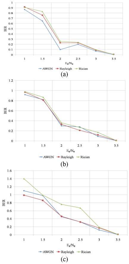
The performance analysis parameter BERdepends upon the modulation format used in the transmission section. The selection of the particular digital modulation format is important to provide error-free data transmission and reception. In case of a wireless image transmission and reception system, small errors in the received medical image create a greater impact on the tumor diagnosis process by the radiologist or physician in the receiving side. Therefore, it is important for choosing the suitable modulation format for the proposed wireless medical image transmission system. Figure 10(a) shows the BER performance illustration graph with respect to the BPSK modulation technique, Figure 10(b) shows the BER performance illustration graph with respect to the QPSK modulation technique, and Figure 10(c) shows the BER performance illustration graph with respect to QAM modulation technique. By comparing all the values of Figure 10, the BPSK modulation format provides less BER on the AWGN channel and higher BER for the Rician channel. In Figure 10(b), the QPSK modulation format provides more or less similar BER values for all AWGN, Rayleigh and Rician channels. In Figure 10(c), the QAM modulation format provides less BER on AWGN channel and higher BER for Rician channel.
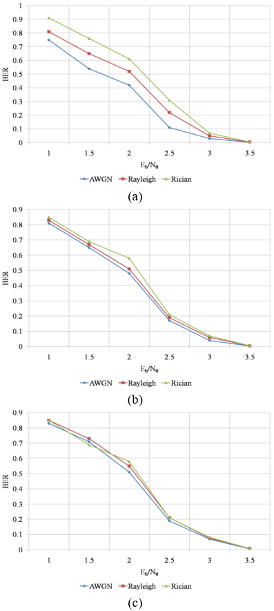
The performance analysis parameter BER is depending upon the encoding technique used in the transmission section. The selection of the particular encoding technique is important to provide error free data transmission and reception. Therefore, it is important for choosing the suitable encoding technique for the proposed wireless medical image transmission system. Hence, its performance analysis is important for error-free transmission through the wireless channels. Figure 11(a) shows the BER performance illustration graph with respect to Convolutional encoding technique, Figure 11(b) shows the BER performance illustration graph with respect to Polar encoding technique and Figure 11(c) shows the BER performance illustration graph with respect to turbo encoding technique.By comparing all the values in Figure 11, the Convolutional encoder provides less BER on AWGN channel and higher BER for Rician channel. In Figure 11(b), the polar encoder provides more or less similar BER values for all AWGN, Rayleigh, and Rician channels. In Figure 11(c), the turbo encoding technique provides less BER on AWGN channel and higher BER for Rician channel.
Figure 11. Bit Error Rate (BER) performance analysis, (a) for convolutional encoding method, (b) for polar encoding method, (c) for turbo encoding method
Table 10. Computational cost and model complexity analysis of the proposed system
|
Computational Cost and Model Complexity |
Values |
|
Training time period |
90 minutes |
|
Inference time period |
10.1 ms/image |
|
Parameters |
3.2 M |
|
FLOPSs |
0.7 GFLOPs/image |
|
Model size |
14 MB |
|
Inference memory requirement |
0.3 GB |
Table 10 shows the computational cost and Model complexity analysis of the proposed system.
Based on the computational cost and model complexity, the proposed system is suitable for practical implementation.
This research article presents the wireless transmission and reception of the brain medical MRI images using MLF-CNN classification methodology. The feature correlation coefficients are obtained using NSCT, and these coefficients are used to construct the multi-level features. These multi-level features are classified by the MLF-CNN, which detects the tumor in the brain MRI. The segmented tumor regions are transmitted by the Convolutional encoder after compression takes place on the tumor images. The experimental results show that the proposed framework, as stated in this article, segments the tumor regions in the brain MRI correctly. Further, the performance of the wireless communication-based transmission and reception system has been analyzed using BER and Eb/N0. Moreover, the BER performances are measured and analyzed with respect to various wireless channels and encoding methods in this article.
The limitations of this research article are stated below.
•The severity levels of the tumor regions in medical images are not performed as identified as the main limitation of this work.
•The various types of noise and their impact on the received signals are not measured in real time.
•Other modality of images is not tested in this work which can improve the performance of the system.
•The various image acquisition procedures will reduce the performance of the end system.
•The proposed work has been tested only on the public datasets and not tested on the clinical dataset as identified as the main limitation of this research work.
The future work of this article is that it identifies the tumor brain images and then transmitted over the channel after compression. This system did not analyze the impact of various medical imaging modalities and medical images over the wireless channels. This is considered future work by extending this research work to find a solution for this.
[1] Amran, G.A., Alsharam, M.S., Blajam, A.O.A., et al. (2022). Brain tumor classification and detection using hybrid deep tumor network. Electronics, 11(21): 3457. https://doi.org/10.3390/electronics11213457
[2] Vimala, M., Palanisamy, S., Guizani, S., Hamam, H. (2024). Efficient GDD feature approximation based brain tumour classification and survival analysis model using deep learning. Egyptian Informatics Journal, 28: 100577. https://doi.org/10.1016/j.eij.2024.100577
[3] Vankdothu, R., Hameed, M.A., Fatima, H. (2022). A brain tumor identification and classification using deep learning based on CNN-LSTM method. Computers and Electrical Engineering, 101: 107960. https://doi.org/10.1016/j.compeleceng.2022.107960
[4] Nayak, D.R., Padhy, N., Mallick, P.K., Zymbler, M., Kumar, S. (2022). Brain tumor classification using dense efficient-net. Axioms, 11(1): 34. https://doi.org/10.3390/axioms11010034
[5] Liao, H., Li, Y. (2024). LC-TMNet: Learned lossless medical image compression with tunable multi-scale network. PeerJ Computer Science, 10: e2511. https://doi.org/10.7717/peerj-cs.2511
[6] Wu, J., Wu, C., Lin, Y., et al. (2024). Semantic segmentation-based semantic communication system for image transmission. Digital Communications and Networks, 10(3): 519-527. https://doi.org/10.1016/j.dcan.2023.02.006
[7] Wen, Z., Fang, J., Wang, X. (2024). A semantic communication model for the task of high quality image transmission to edge-end devices. Internet of Things, 28: 101384. https://doi.org/10.1016/j.iot.2024.101384
[8] Li, S., Lu, J., Hu, Y., Mattos, L.S., Li, Z. (2025). Towards scalable medical image compression using hybrid model analysis. Journal of Big Data, 12(1): 45. https://doi.org/10.1186/s40537-025-01073-1
[9] Dai, F. (2025). Deep learning based medical image compression using cross attention learning and wavelet transform. Scientific Reports, 15(1): 40008. https://doi.org/10.1038/s41598-025-23582-y
[10] Asif, R.N., Naseem, M.T., Ahmad, M., et al. (2025). Brain tumor detection empowered with ensemble deep learning approaches from MRI scan images. Scientific Reports, 15(1): 15002. https://doi.org/10.1038/s41598-025-99576-7
[11] Ahmed, M.M., Hossain, M.M., Islam, M.R., et al. (2024). Brain tumor detection and classification in MRI using hybrid ViT and GRU model with explainable AI in Southern Bangladesh. Scientific Reports, 14(1): 22797. https://doi.org/10.1038/s41598-024-71893-3
[12] Rao, K.N., Khalaf, O.I., Krishnasree, V., et al. (2024). An efficient brain tumor detection and classification using pre-trained convolutional neural network models. Heliyon, 10(17): e36773. https://doi.org/10.1016/j.heliyon.2024.e36773
[13] Abdusalomov, A.B., Mukhiddinov, M., Whangbo, T.K. (2023). Brain tumor detection based on deep learning approaches and magnetic resonance imaging. Cancers, 15(16): 4172. https://doi.org/10.3390/cancers15164172
[14] Khairandish, M.O., Sharma, M., Jain, V., Chatterjee, J.M., Jhanjhi, N.Z. (2022). A hybrid CNN-SVM threshold segmentation approach for tumor detection and classification of MRI brain images. IRBM, 43(4): 290-299. https://doi.org/10.1016/j.irbm.2021.06.003
[15] Zhang, J., Jiang, Z., Dong, J., Hou, Y., Liu, B. (2020). Attention gate Resu-Net for automatic MRI brain tumor segmentation. IEEE Access, 8: 58533-58545. https://doi.org/10.1109/ACCESS.2020.2983075
[16] Vikraman, B.P., Afthab, J. (2024). Effective image compression using hybrid DCT and hybrid capsule auto encoder for brain MR images. Journal of Visual Communication and Image Representation, 104: 104296. https://doi.org/10.1016/j.jvcir.2024.104296
[17] Seenuvasamurthi, S., Ashok, S., Shankarlal, B., Abbas, A.M., Vajravelu, A. (2024). Brain image compression and reconstruction system using deep learning. International Journal of Medical Engineering and Informatics, 16(5): 401-413. https://doi.org/10.1504/IJMEI.2024.140799
[18] Nickparvar, M. (2020). Brain Tumor MRI Dataset. Kaggle Dataset. https://doi.org/10.34740/kaggle/dsv/14832123
[19] Cheng, J. (2022). Brain Tumor Dataset. V1. Science Data Bank. https://doi.org/10.57760/sciencedb.06290
[20] Khan, S.U.R., Asif, S., Zhao, M., Zou, W., Li, Y., Xiao, C. (2026). ShallowMRI: A novel lightweight CNN with novel attention mechanism for Multi brain tumor classification in MRI images. Biomedical Signal Processing and Control, 111: 108425. https://doi.org/10.1016/j.bspc.2025.108425
[21] Naeem, A.B., Osman, O., Alsubai, S., Cevik, T., Zaidi, A., Rasheed, J. (2025). Lightweight CNN for accurate brain tumor detection from MRI with limited training data. Frontiers in Medicine, 12: 1636059. https://doi.org/10.3389/fmed.2025.1636059
[22] Raza, A., Iqbal, M.J. (2025). Lightweight-CancerNet: A deep learning approach for brain tumor detection. PeerJ Computer Science, 11: e2670. https://doi.org/10.7717/peerj-cs.2670