Sivakumar Madeshwaran* | K. Devaki
© 2026 The authors. This article is published by IIETA and is licensed under the CC BY 4.0 license (http://creativecommons.org/licenses/by/4.0/).
OPEN ACCESS
The diagnosis of Parkinson's disease (PD) in its early stages is crucial for timely intervention and cost-effective treatment. Existing methods may lack accuracy and efficiency in detecting PD in its initial phases, leading to delayed diagnosis and treatment initiation. Current approaches for PD diagnosis may suffer from limitations such as insufficient sensitivity, specificity, or reliance on subjective assessments. Additionally, some methods may not leverage advanced machine learning techniques, potentially hindering their ability to discern subtle patterns indicative of early-stage PD. This paper presents a cloud-based machine learning diagnostic system designed to analyze patient voice data for early PD detection. The system employs a combination of random forest (RF) and bidirectional long short-term memory (Bi-LSTM) machine learning techniques alongside a Maximized Mutual Information (MMI) feature selection method. This amalgamation aims to improve the accuracy and reliability of PD diagnosis during the initial stages. In the subsequent phase, the best diagnostic model is deployed in cloud computing, and an Android application is developed to serve as the interface for this diagnostic model. To manage outliers, a grid-based fuzzy one-class support vector regression is incorporated at both the physical and abstraction layers of the cloud. Evaluation metrics such as accuracy, F1-score, recall, and precision are used to evaluate the classification models' performance. The performance of the six machine learning models is assessed on the dataset both before and after hyperparameter tuning. Results indicate that the proposed random forest–bidirectional long short-term memory–maximized mutual information (RF-BiLSTM-MMI) model outperforms other classification methods, achieving an accuracy of 93.4%, an F1-score of 93.6%, a recall of 94.3%, and a precision of 93.5%. These results demonstrate the effectiveness of the proposed framework for early PD detection using voice signals.
Parkinson’s disease, cloud infrastructure, voice analysis, mutual set, outlier handling, hyperparameter
Neurodegenerative disorders, most notably Parkinson's disease (PD), pose a significant threat to the elderly population, which includes people aged 50 and beyond. This population is particularly susceptible to the severe effects of these conditions [1]. Because PD affects neurological issues, it affects gradual loss of control over the muscles. The presence of genetic variables has been identified as a key contribution to PD [2]. The characteristic tribulation dementia that is seen in PD patients highlights the vital need to receive therapy in an early manner. Despite the fact that research is still being conducted, there is still a noticeable void in the field. This calls for a detection method that is both more accurate and more easily available, and it would be perfect if it were in the form of a mobile application [3].
In this study, a cloud-based strategy is recommended for early PD detection. The goal of using AI techniques with Parkinson's statistics is to reduce the dimensionality of the data via selecting characteristics while continuously maximising the efficiency of classification. For the purpose of determining which method of PD diagnosis is the most efficient, it is essential to use classification algorithms such as random forest (RF) and bidirectional long short-term memory (Bi-LSTM) along with Maximized Mutual Information (MMI) feature selection. Then, grid-based fuzzy one-class support vector regression is accelerated to preserve the privacy of the medical data. These algorithms are then put through extensive training and testing. Cloud computing, which has the ability to provide unrestricted access to computer resources under favourable conditions [4], is an essential component of this strategy. With the assistance of the cloud, the enormous amount of data is properly saved and managed in an economical manner.
Cloud computing offers characteristics such as scalability, stability, and storage, which make it easier to manage large amounts of data. This is in recognition of the fact that significant security measures are required when dealing with this data in order to prevent corruption and malicious activity. The most significant accomplishment of this study is the creation of an automated PD diagnostic platform that includes a smartphone application. After presenting the results regarding performance assessments, the next sections will provide a detailed review of earlier studies, expound on the suggested method for diagnosing PD and its intricate design, and conclude with some last observations. The main innovation of the study is the incorporation of cutting-edge data mining methods into a cloud-based diagnostic application for speech analysis-based early PD identification. The key contributions include:
•This research combines RF and Bi-LSTM models, offering a synergistic approach that leverages the strengths of both techniques. This fusion enhances the ability to capture subtle patterns indicative of early-stage PD in patient voice data.
•The use of MMI-based feature selection optimizes the selection of relevant features, ensuring that the diagnostic model is built upon the most informative subset. This contributes to the accuracy and reliability of the PD diagnosis in its initial stages.
•The incorporation of a grid-based fuzzy one-class support vector regression at both the physical and abstraction layers of the cloud addresses the challenge of outliers, enhancing the robustness of the diagnostic system in real-world scenarios.
•The thorough evaluation and optimization of six machine learning models pre- and post-hyperparameter tuning contribute to achieving the outstanding accuracy of 93.4%, showcasing the effectiveness of the proposed model.
The subsequent sections are structured in the following manner: Detailed information regarding the background of the work and the proposed work’s highlights in Section 2, which provides a complete assessment of research that has utilised machine learning approaches in the identification and classification of PD. For the purpose of performing PD categorization, Section 3 provides an overview of the suggested feature selection process that incorporates fault tolerance in the cloud context. Section 4 evaluates the suggested technique and compares it to existing machine learning methods for PD classification. Summary of research results and conclusions in Section 5.
PD is a progressive neurodegenerative disorder with both motor and non-motor symptoms. One of its early signs is voice impairment, which can be picked up as a biomarker [5]. Analysing voice signals allows us to spot these issues without invasive procedures. By looking at things like jitter, shimmer, harmonics-to-noise ratio (HNR), and changes in fundamental frequency, we get valuable acoustic features [6].
Scientists often use the UCI Parkinson's Speech Dataset to build their models. They clean the data, handle class imbalance with SMOTE, and then apply different classifiers like RF [7], Extreme Gradient Boosting (XGBoost) [8], SVM [9], and multilayer perceptrons [10]. These models usually achieve accuracy rates over 95%. One really useful technique in boosting these models' performance is MMI feature selection. It figures out how each feature relates to the outcome, helping to cut down on extra dimensions and noisy data. Plus, when you combine this method with recursive feature elimination (RFE) [11], the model gets more robust and works well under different recording conditions. Key biomarkers that pop up a lot include MDVP:Fo(Hz), various types of shimmer [12], spread1, spread2, and PPE. These indicators suggest problems with the voice tied directly to PD. Compared to older methods like ANOVA [13] or Chi-squared, mutual information filtering performs way better in complex scenarios [14]. Researchers usually see higher precision, recall, and AUC when they fine-tune parameters with GridSearchCV or Bayesian optimization [15]. Narrowing it down to important features not only stops overfitting but also speeds up the process and aids generalization [16]. There are still some hurdles, though, mainly in getting these voice systems ready for real-life predictions. Specifically, pulling off feature extraction, selection, and analysis efficiently on huge datasets is tricky. But cloud technology can fix many of these issues [17-21]. It gives flexible access to computing power and secure storage, and makes deploying machine learning pipelines easier [22].
Through apps on smartphones, patients can easily upload their voice samples [23]. Then, these uploads go through preprocessing and analysis by the system in place. On top of that, this tech supports remote health care even in areas with limited resources, all while keeping data private and compliant with regulations [24, 25]. Combining feature selection and smart cloud setups is key to spotting PD early on. Streamlining the number of features makes the whole analysis quicker and lets the system zoom in on significant patterns [26]. Long-term tracking of voice changes becomes possible too, aiding early interventions [27].
Of course, there's still room for improvement, especially in making models work across languages and handling variations in recordings [28-31]. Maybe in the future, PD prediction could combine voice data with info on walking or brain scans. And researchers should definitely look into protecting patient privacy and creating models [32] that doctors find easy to understand. To sum up, putting advanced feature selection with intelligent cloud setups together is a game-changer. It helps create an accurate, wide-reaching system for catching PD early through analysing voice.
While the comprehensive survey provides valuable insights into various approaches for PD analysis and prediction using ML and DLs, there are several research gaps and areas where further investigation could enhance the existing knowledge:
•Most studies focus on a specific data modality such as movement, handwriting, or voice. Investigating the integration of several data sources to raise the precision and resilience of PD forecasting techniques may represent a research need.
•While motor symptoms are commonly utilized for PD diagnosis, there is a need to explore and incorporate non-motor symptoms such as sensory dysfunction, sleep difficulties, and changes in voice. Integrating these less overt symptoms into predictive models could contribute to early and accurate diagnosis.
•While several studies propose promising models, there is a gap in real-world cloud deployment and validation without compromising the confidentiality of these models in clinical settings.
•Recent advances in deep learning, particularly Transformer-based architectures and attention mechanisms, have demonstrated promising performance in speech analysis tasks. However, their application to cloud-based PD diagnosis using voice signals remains limited. Future investigations should compare Transformer-based approaches against conventional machine learning and recurrent neural network architectures.
•Existing studies rarely investigate end-to-end cloud-enabled diagnostic platforms integrating feature selection, classification, deployment, privacy preservation, and mobile accessibility within a unified framework as in Table 1. This research attempts to address this gap through a cloud-based random forest–bidirectional long short-term memory–maximized mutual information (RF-BiLSTM-MMI) model diagnostic architecture.
Table 1. A comparative analysis of Parkinson's disease (PD) diagnostic methods
|
Ref. No. |
Tech Used |
Numeric Outcomes |
Advantages |
Disadvantages |
|
[5] |
Acoustic feature extraction + ML classifiers (RF, SVM, etc.) |
Accuracy: ~95-98% |
Non-invasive, easy data collection |
Limited to controlled recordings, lower generalizability |
|
[6] |
Fine-tuned ML/DL classifiers on vocal features |
Accuracy: up to 97%, AUC: 0.96+ |
High precision on vocal characteristics |
Computationally intensive for DL models |
|
[7] |
ML system on speech signals (various classifiers) |
Accuracy: 90-95% |
Robust feature extraction from speech |
Small dataset size, overfitting risk |
|
[8] |
Feature selection + hyperparameter tuning with ML |
Accuracy: >96% with optimized FS |
Improved diagnosis via efficient tuning |
Depends heavily on dataset quality |
|
[9] |
ML approaches with voice signal features + SMOTE |
Accuracy: up to 98.31% |
Handles class imbalance effectively |
May not generalize across languages/accents |
|
[10] |
Feature selection (mRMR, others) for speech-based diagnosis |
Improved accuracy by 3-5% post-FS |
Reduces dimensionality effectively |
Requires careful threshold selection |
|
[11] |
Efficient ML on voice signals (SVM, RF, XGBoost) |
Accuracy: 94-97% |
Fast inference suitable for real-time |
Sensitive to noise in recordings |
|
[12] |
Evolutionary algorithms + vocal feature analysis |
Accuracy: ~95%, good classification rates |
Optimizes feature subsets globally |
High computational cost for evolution |
|
[13] |
Hybrid feature selection (MI, F-score, Chi-square) |
Superior performance with ensemble FS |
Flexible and extensible framework |
Complex hybridization increases overhead |
|
[14] |
Cloud-based framework with voice analysis + ML |
High detection accuracy in remote settings |
Scalable for low-resource areas |
Privacy and data security concerns |
|
[15] |
Hybrid MI gain + RFE for PD detection |
Enhanced accuracy and reduced features |
Balances relevance and redundancy |
Wrapper methods can be slow |
|
[16] |
SMOTE + FS methods (ANOVA, MI, Chi-squared) |
Significant performance boost with MI |
Optimizes PD detection from voice |
Performance varies with FS technique |
|
[17] |
Non-invasive speech recordings + acoustic features |
High sensitivity/specificity (~95%) |
Accessible screening method |
Variability in recording conditions |
|
[18] |
System-based voice features + classifiers |
Improved detection rates |
Focus on robust features |
Limited multimodal integration |
|
[19] |
MI-based Cuckoo Search optimization + classifiers |
Better accuracy than baselines |
Efficient global optimization |
Metaheuristic may require tuning |
|
[20] |
Hybrid FS based on MI and AUC |
Accuracy improvement of 4-7% |
Effective relevance filtering |
AUC computation adds overhead |
|
[21] |
Fog computing + cyber-physical system for PD detection |
Reduced latency in detection |
Edge processing benefits |
Infrastructure dependency |
|
[22] |
ML and DL (CNN, RNN) on voice data |
Accuracy: 96-98% with DL |
Handles complex patterns |
Requires large training data |
|
[23] |
Supervised ML on voice recordings |
Early detection with high recall |
Simple and interpretable |
Lower performance on noisy data |
|
[24] |
Comprehensive vocal parameter analysis + ML |
Strong predictive performance |
Thorough feature exploration |
High feature dimensionality |
|
[25] |
Different FS techniques on voice datasets |
Varies; MI often best |
Supervised learning focus |
Dataset-specific results |
|
[26] |
Comparative voice analysis techniques |
Optimized prediction models |
Identifies best practices |
Comparative nature limits novelty |
|
[27] |
FPGA prototype with voice analysis |
Efficient hardware acceleration |
Low-power real-time detection |
Hardware-specific, less flexible |
|
[28] |
Cloud framework for remote monitoring |
Scalable telemonitoring |
Enables global access |
Network dependency and latency |
|
[29] |
Mobile-assisted voice analysis system |
Good accuracy in field tests |
Portable and user-friendly |
Battery and device limitations |
|
[30] |
Telemonitoring with ML on tremors/voice |
Effective discrimination |
Longitudinal tracking |
Data synchronization issues |
|
[31] |
Hybrid MI-RFE for vocal FS |
Enhanced classification metrics |
Strong redundancy reduction |
Computation time for RFE |
|
[32] |
AI-powered pangram/speech analysis |
High screening accuracy (~97% UAR/AUC) |
Natural speech analysis |
Domain-specific language constraints |
Note: ML = Machine Learning; DL = Deep Learning; AI = Artificial Intelligence; RF = Random Forest; SVM = Support Vector Machine; XGBoost = Extreme Gradient Boosting; SMOTE = Synthetic Minority Over-Sampling Technique; mRMR = Minimum Redundancy Maximum Relevance; MI = Mutual Information; RFE = Recursive Feature Elimination; FS = Feature Selection; ANOVA = Analysis of Variance; AUC = Area under the Receiver Operating Characteristic Curve; CNN = Convolutional Neural Network; RNN = Recurrent Neural Network; FPGA = Field-Programmable Gate Array; UAR = Unweighted Average Recall.
In a description of the primary components of the article, which include the feature selection technique and ML algorithms for classification, as well as the specifics of the needs for cloud computing. It involves identifying the optimal subset of features (m) from a pool of (M) features, excluding redundant or irrelevant ones. This process streamlines system complexity and computational time.
The MMI attribute selection technique is used in this work. By choosing a subset (m) that successfully separates target labels determined by data that is shared, MMI seeks to find relevant characteristics. The following outlines the MMI feature selection approach.
To find out how much information is shared among two independent random variables (x and y), you use their individual potential outcomes (P(x), P(y)) and their joint proportion (P(x, y)) [33-35].
$I\left( X,Y \right)=\underset{x\in X}{\overset{n}{\mathop \sum }}\,\underset{y\in Y}{\overset{n}{\mathop \sum }}\,p\left( x,y \right)\log \left( \frac{p\left( x,y \right)}{p\left( x \right)p\left( y \right)} \right)$ (1)
Here, x stands for a particular attribute selected from the collection of features X, and y is the class identifier found in the set of templates Y.
|
Algorithm 1: Feature selection (FS) based on Maximized Mutual Information (MMI) |
|
I/P: Database ($\boldsymbol{X}$,). |
When two traits are highly dependent, removing one does not appreciably affect their discriminative power. Finding the smallest collection of features (S) with characteristics {xi} (n total) that show the highest dependence on the target class y while minimising duplication among them is the aim of the MMI approach. Method 1's Python-implemented MMI feature selection method seeks to accomplish this. The maximisation of dependence among the variable xiwith label y is shown in Eq. (2). Meanwhile, Eq. (3) shows how to minimise dependence among features (xi and xj), acting as an amplifier for incompatible characteristics.
$MaxRv\left( {{x}_{i}},y \right)=\frac{1}{m}\underset{{{x}_{i}}s\in }{\overset{n}{\mathop \sum }}\,l\left( {{x}_{i}},y \right)$ (2)
$MinRd\left( {{x}_{i}},{{x}_{j}} \right)=\frac{1}{m}\underset{{{x}_{i~xj}}\in s}{\overset{n}{\mathop \sum }}\,l\left( {{x}_{i}},{{x}_{j}} \right)$ (3)
It uses a progressive searching procedure to find the probable optimum set of characteristics S, as shown in Eq. (5).
$max\varphi \left( Rv,Rd \right),\varphi =Rv-R$ (4)
$\max _{x j \epsilon-s m-1}\left[l\left(x_i, y\right)-\frac{1}{m-1} \sum_{x i \epsilon s m-1} l\left(x_i, x_j\right)\right]$ (5)
This research uses MMI to reduce data attributes while keeping good accuracy after learning the classification model with the chosen features. This process involves eliminating irrelevant features that could otherwise confuse the classification model's decision-making process, ultimately affecting accuracy. Furthermore, removing redundant features helps decrease the overall complexity.
Clinical Significance of Selected Features: The MMI feature selection process prioritized features exhibiting the strongest dependency on PD status while minimizing redundancy among features. Several selected attributes have established clinical relevance. Jitter-related parameters reflect cycle-to-cycle frequency instability caused by impaired vocal fold control. Shimmer measures amplitude perturbations associated with neuromuscular dysfunction. Harmonic-to-Noise Ratio (HNR) and Noise-to-Harmonic Ratio (NHR) capture breathiness and vocal roughness commonly observed in PD patients. Nonlinear measures such as RPDE, DFA, Spread1, Spread2, D2, and PPE characterize abnormalities in vocal dynamics and phonatory control. These features collectively represent known manifestations of Parkinsonian speech impairment, supporting the clinical relevance of the selected feature subset.
3.1 Utilizing machine learning models for classification
Working as an Artificial Intelligence (AI) tool, the classifier divides input data into a number of predetermined classes (k). Its main goal is to correctly identify test samples with the least amount of information and characteristics. The hybrid RF-BiLSTM architecture was selected to exploit the complementary strengths of both learning paradigms. RF effectively captures nonlinear relationships among engineered voice features and provides robustness against noise and overfitting. In contrast, Bi-LSTM models’ temporal dependencies and sequential patterns present in voice signals that may not be captured by conventional machine learning algorithms. The integration of both models enables simultaneous learning of statistical feature interactions and temporal speech dynamics. Final predictions are generated through ensemble decision fusion, where outputs from both models are combined to improve classification stability and diagnostic accuracy.
This research uses two different AI methodologies, which are as follows:
3.1.1 Bidirectional long short-term memory integration
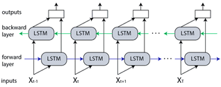
The long short-term memory (LSTM) belongs to the category of artificial recurrent neural networks, commonly applied in deep learning. Known for its ability to retain data over extended periods, LSTM finds utility in data prediction and classification tasks. LSTM have four layers: an input layer, two concealed, and a final outlet. The first figure shows their fundamental components.
LSTM architecture incorporates specialized memory blocks known as cells, where data is stored and managed through elements termed gates. The forget gate determines what information to retain or discard within the cell. It calculates the relevance of the previous states in relation to the current state. Meanwhile, the input gate controls the addition of pertinent information to the cell state, which is eventually extracted for output or passed on to subsequent cells through the output gate.
1) Forget gate: In initial stage within LSTM involves the forget gate determining whether to retain the information from the cell. The outcome of this forget gate, denoted as bf in Eq. (6).
${{f}_{t}}=\sigma ({{w}_{f}}\left[ {{h}_{t-1}},{{x}_{t}} \right]+{{b}_{f}}$ (6)
In this case, $\sigma $ stands for the sigmoid function, whereas wf and ht-1 are the weighted matrices connected to the forget gate. Furthermore, the bias is denoted by bf, and the input characteristics used in the calculation are indicated by xt.
2) Input gate: The next step is to save fresh data in the cell state using the output of the input gate, as computed in Eq. (7). This procedure begins by upgrading the cell memories with alternative principles, as shown in Eq. (8).
$i_t=\sigma\left(w_i\left[h_{t-1}, x_t\right]+b_i\right)$ (7)
$C=\tanh \left(w_c\left[h_{t-1}, x_t\right]+b_c\right)$ (8)
Here, wi and wc denote the weights associated with the input level while ${{h}_{t-1}}$ and ${{x}_{t}}$ represent the bias to their corresponding incoming gate. Additionally, tanh represents the activation function employed in the process.
3) Cell state: At the current time step, the cell state is identified by multiplying the forget gate by the current state, then adding the resultant of the input gate elements, as shown in Eq. (9).
${{c}_{t}}={{f}_{t}}*{{c}_{t-1}}+{{i}_{t}}*c$ (9)
'it' here indicates the input gate's output, 'c' the cell state, 'ct−1' the condition of the cell prior to now, and 'ct' the current cell state.
Completing the procedure for making choices within the resultant gate, as shown in Eq. (12), is the last stage. To do this, run the initial output—which was previously determined in Eq. (10), over the sigmoid activating function, as shown in Eq. (11).
$o_t=\sigma\left(w_o\left[h_{t-1}, x_t\right]+b_o\right)$ (10)
${{h}_{t}}={{o}_{t}}\tanh ({{c}_{t}})$ (11)
$outpu{{t}_{class}}=\sigma \left( {{h}_{t}}*{{W}_{out~parameter}} \right)$ (12)
Here, ${{W}_{o}}$ and ${{W}_{out~parameter }}$represent the weights associated with the output gate, while bo signifies the bias term. Additionally, $Outpu{{t}_{class}}$ denotes the classification outcome and stands for the sigmoid activated function used in this process.
3.1.2 Random forests integration
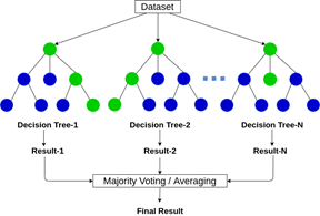
Among the data extraction methods used mostly for supervised training is RF. It constructs a 'forest' by generating multiple decision trees through a technique called 'bagging,' where each tree is trained independently to enhance classification accuracy, as shown in Figure 1.
By building numerous categorical decision chains throughout learning, RF is used in regression, classification, and other applications. The essential characteristics of RF are:
•Handling multiclass classification and regression naturally.
•Swift training and prediction.
•Dependency on one or two factors for tuning.
•Built-in estimation of generalized fault.
•Applicability to high-dimensional problems.
•Feasibility for parallel implementation.
•Capability to measure variable importance.
•Support for differential class weighting.
•Unsupervised learning with potential for visualization and outcome received.
Figure 1. Framework for bidirectional long short-term memory (Bi-LSTM) network
The operational steps of RF can be summarized as below:
Examine a collection of real-value inputs for their variables X = X1 ….. Xp that have 'p' values.
$E_{x y}=(L,(Y, f(x)))$ (13)
Here, $\left( Y,f\left( X \right) \right)$ denotes the loss function utilized for computing the predictive function $f\left( X \right)$, where 'Y' stands for the actual outcome. The common representation of the loss function is through the root mean square error. However, in RF classifiers, the entropy information gain often serves as the default loss function.
$L(Y, F(X))=I(Y \neq F(X))=\left\{\begin{array}{c}0 \text { if } Y=F(X) \\ 1 \text { otherwise }\end{array}\right.$ (14)
The potential range of 'Y' are encompassed within the real number space (ℝ). EXY (L(Y, f(X))), particularly for 0 – 1 loss, yields the Bayes rule as depicted in Eq. (15).
$f\left( x \right)=argma{{x}_{y\in R}}P(Y=y|X=x)$ (15)
Eq. (16) shows how the collective prediction 'f,' which includes hj(x) base learners, votes to decide the projected class.
$f\left( x \right)=argma{{x}_{y\epsilon R}}\underset{j=1}{\overset{J}{\mathop \sum }}\,I\left( y={{h}_{j~}}\left( x \right) \right)$ (16)
Here, 'Y' stands as the RF denoting the output, while $X$ represents the predictive function used for estimating Y. $EXY$ signifies the loss of outcome, with ℝ denoting the possible values of Y. Additionally, $h_j~\left( x \right)$ corresponds to the jth base within the ensemble.
3.2 GAE: Google application engine
In 2008, the introduction marked Google's entry into the demand-driven computing market by giving users access to a framework that allows them to create and host a variety of web-based apps within its data facilities. This service became publicly available in November 2011 alongside other cloud services provided by Google. GAE essentially functions as a comprehensive file system, providing users with more extensive capabilities than a standard engine, including read/write permissions. GAE standard users have a fixed set of libraries in serverless technology settings, restricting third-party library distribution. Representational State Transfer (REST) serves as a web service design architecture and stands as a popular alternative to SOAP. REST is favoured for its lower bandwidth consumption, making it a preferred choice for internet usage. SOAP operates on a client/server logic protocol using the RPCs model, resulting in services becoming XML documents that define the methods for calling. Because XML is used in SOAP exchanges often, greater storage capacity is used. REST sends information in XML or JSONs forms to the website's server via requests made over HTTP. Cloud-based APIs from Google, Amazon, Twitter, and Ms choose REST owing to its flexibility and inexpensive construction. A web service that uses the REST framework is known as a RESTful API in Figure 2.
Figure 2. Framework for random forest (RF)
3.3 Parkinson's disease diagnosis process in cloud environment
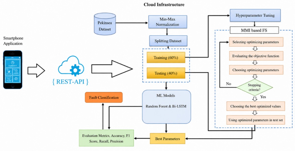
Utilising a cloud-hosted environment is how the PD screening system operates. A visual depiction of the elements and setup of the cloud-based PD detection platform is shown in Figure 3. The cloud-powered ML-based PD diagnostic technique, the RESTful API, and the Google Play mobile app have been recognised as the method's three key elements.
Figure 3. Overall flow of the proposed taxonomy
3.3.1 Cloud deployment phase
The machine learning methodology that has been proposed for the development of the PD detection system combines many distinct elements. These consist of the PD evaluation database, the initial processing stage, which is in charge of getting the information set ready for training the machine developing categorization approach, the feature identification stage, which lowers dimensions by selecting the best characteristics that show exceptional performance in task categorising, and the algorithms used for machine learning phase. In the last stage, a number of different ML algorithms get trained by making use of the data that was collected in the stage before it. Subsequently, the model's capacity for classification is calculated to determine the most efficient approach for creating a model for categorization appropriate for PD identification.
The data used in this study regarding PD were gathered by Max Minor from the University of Cambridge and the National Centre of Voice [14]. This dataset contains information derived from voice recordings of 32 individuals. Among them, 24 have a diagnosis of PD, while the other 8 are considered to be in good health. There are an overall of 195 recordings of voices included in the dataset, and each recording produces 22 retrieved features, as summarised in Table 2. The extraction of these traits is accomplished either through prolonged vowel phonation or through a running voice test [20]. Individuals are asked to articulate the vowel "a" for a period of time that is shorter than ten seconds while using lab microphones and recording tools. This technique is known as sustained vowel phonation. Each recording is linked to a binary PD score for the purpose of prediction. The benchmark data that was accessed from the ML data collection in reference [21] was the database that was utilised for this researcher's investigation. For practical deployment, the proposed system was implemented using Google Application Engine, which provides automatic resource scaling and high availability. The average audio recording duration is limited to 10 seconds, resulting in relatively low bandwidth requirements during transmission. Since only extracted acoustic features are transmitted to the cloud rather than raw continuous audio streams, communication overhead is minimized. Preliminary testing indicated response times suitable for near real-time diagnosis. Future studies will include detailed latency analysis, cloud resource utilization measurements, and cost evaluation under large-scale clinical deployment scenarios.
Table 2. 22 feature sets
|
No |
Attributes |
|
1-3 |
Multi-Dimensional Voice in normal (MDVP) |
|
4 |
Percentage of Multi-Dimensional Voice |
|
5 |
Multi-Dimensional Voice in abs |
|
6-8 |
DDPs, RAPs, PPQs |
|
9-10 |
Shimmer in dBs |
|
11-12 |
APQs |
|
13 |
MDVPs |
|
14 |
DDAs |
|
15-16 |
NHRs by HNRs |
|
17-18 |
RPDEs |
|
19 |
DFAs |
|
20-21 |
Spreading of 1-2 |
|
22 |
PPEs |
Note: MDVP = Multi-Dimensional Voice Program; NHR = noise-to-harmonics ratio; HNR = harmonics-to-noise ratio.
Within the scope of this investigation, each of the 22 characteristics is addressed. It is possible to aggregate the values that correspond to these characteristics for an identical person by employing functions such as the minimum, the range, the standard deviation, the mean, and the maximum. The combining process is carried out in an iterative manner for each participant, which ultimately results in an information set size of 32 by 110 measurements. It has been decided that the set number of features for the MMI algorithm will be (5%, 10%, 25%, 50%, 75%, and 100%), correspondingly.
It is important to divide the classification data into two or more sets in order to get it ready for use. When the classifier is being trained, one set is utilised for training, and this set will be referred to as the set for training. Another set, which is additionally referred to as the test set, is used to evaluate whether or not the classifier has successfully learnt the rules.
3.3.2 Utilization of the application programming: RESTful
The smartphone or tablet and the PD assessment that is located in the cloud are connected through the RESTful Interface for Application Programming (API), which acts as a connection between the two. The Flask Python toolkit is utilised in order to develop and put in the RESTful API that is hosted in the cloud. POST is a mechanism that is utilised within the mobile application to submit patient information to the Bi-LSTM PD detection model that is located in the cloud, receive the forecast outcome & then send it again to the app. In Algorithm 2, the process of calling the RESTful API is described in some detail. The API is put through testing by sending an instance of patient information to CCs. This is done to confirm that the RESTful API that has been created and installed in Google Cloud is running correctly and that it is able to facilitate the required interaction with the mobile application.
|
Algorithm 2: Cloud powered Parkinson's disease (PD) prediction
|
|
I/P: Patient sound features
O/P: PD prediction
1: Initialize and load the LSTMs model (refer to Algorithm 1).
2: Wait for an app request.
3: If info is received:
4: Retrieve data using REST API GET.
5: Proceed to Model Prediction.
6: Else:
7: Return to waiting for an application request.
8: Model Prediction:
9: Perform PD prediction using the loaded model on the received info.
10: Sending their model decision.
11: Transmit results using RESTful API POSTs.
12: Return request from app
|
3.3.3 Smartphone app development phase
This Android mobile software was created to diagnose Parkinson's illness, and it has a simple GUI and is built in Java. The individual can capture audio recordings using the attached recording button in order to aid in the diagnosis of Parkinson's illness. The final test result is then displayed on the screen by the application when you have completed the process. The diagnosis model utilizing machine learning, deployed on Google's cloud infrastructure, is responsible for generating the decision. For more specifics about this cloud-based model for diagnosing PD, refer to Algorithm 2. Additionally, Algorithm 3 outlines the pseudocode for the mobile application related to this diagnosis system.
The mobile app prompts patients to record their sound by articulating the note /a/ three times within a ten-second interval. Praat, derived from the Dutch word for "talk," refers to a sound analysis program. It's employed to recognize sound characteristics akin to those utilized in developing the LSTM diagnosis model.
After the recording of the audio sample, the smartphone app communicates with the Praat software service. After the features have been retrieved, they are translated into the JSON format in order to guarantee compliance with the RESTful API. The cloud-based PD assessment model receives this information after it has been submitted to it.
|
Algorithm 3: Android based Smartphone app
|
|
I/P: sampling of Sound
O/P: PDs evaluation
1: Wait for user action.
2: If the record button is pressed, proceed to Start Recording.
3: Else, return to waiting for user action.
4:
Start Recording:
5: Start the recorder.
6: Wait for 10 seconds.
7: Stop the recorder.
8: Save the recorded file.
9: Perform evaluation of sound.
10: Initial the Praat service.
11: Open the sound file with Praat.
12:
Preparing the Data:
13: Formatted the sound features to JSON (Data).
14: Submit info to the cloud MLs.
15: Utilize RESTful API to POST the info.
16: Receive the model decision from the cloud.
17: Utilize RESTful API to GET the results.
18: Display the results.
19: If the result is negative:
20: Display "The patient does not have PDs."
21: If the result is positive:
22: Display "The patient has PDs."
23: Return to waiting for user action.
|
3.3.4 Outliers control using grid-based fuzzy one-class SVR
A cloud-based web application with flaws has been developed by creating a simulated environment with many nodes using a hypervisor to construct virtual machines. Finding the broken node is essential to getting reliable defective data. The cloud data system archives the tasks allocated to these virtual nodes, while the cloud master maintains control of the virtual servers that are produced. Finding malfunctioning nodes is made easier by analysing data from both sources. In order to efficiently obtain false data, procedures such as pulse tactics, contact plans, keep-alive approaches, and intrusion methods are used. Training data is obtained by using a grid-based fuzzy one-class support vector regression for outlier detection.
Cloud systems can have a variety of issues that originate from software, hardware, and other barriers. Network, process, and data failures are additional categories for software errors. The data must be categorised and trained appropriately in order to create an efficient detection and diagnosis model. Training data is classified as a consequence of the fault classification process using the Bi-LSTM technique. A resource-efficient statistical methodology called logistic regression is used to identify faults. This approach is appropriate for the prediction task because it doesn't require a lot of processing power (Algorithm 4).
${{Y}_{i}}={{\alpha }_{0}}+~{{\alpha }_{1}}{{x}_{i}}+~{{\pi }_{i}}$ (17)
where,
i represents the dependent variable.
${{\alpha }_{0}}$ denotes the population y-intercept.
${{\alpha }_{1}}$ signifies the population slope coefficient.
${{x}_{i}}~$stands for the independent variable.
${{\pi }_{i}}$ represents the random error term.
|
Algorithm 4: Outlier prediction |
|
Load the dataset "test_data.csv" and designate it as 'Test.' Generate a descriptive summary of the 'Test' file using the describe() function. Apply the encoder to transform categorical variables in 'Testcat' using the cattest dataset. Concatenate the scaled 'Test_x' dataframe with the encoded 'enctest' dataframe along the axis. If 'Test_x' meets certain criteria: Return the label "normal." Else, categorize it as "anomaly." Identify selected features based on the conditions specified in the feature_maps, storing them in 'Selected_features.' Evaluate the accuracy and precision of the model. Display the calculated accuracy and precision values. |
The assessment procedure starts with entering the data to be evaluated, reviewing the file, and then providing an explanation of the test data using the SVR (Eq. (17)). By utilising an encoding tool, the test data is converted. The system next performs a critical phase in which it determines if the given data is considered anomalous or typical. The next step is feature extraction, which selects pertinent features. Next, the precision and accuracy of the provided data are ascertained by utilising the logistic regression method. Notably, SVR is applied only to the significant features that are extracted with the help of Bi-LSTM. Calculated results indicate that the accuracy obtained by using logistic regression is 0.981.
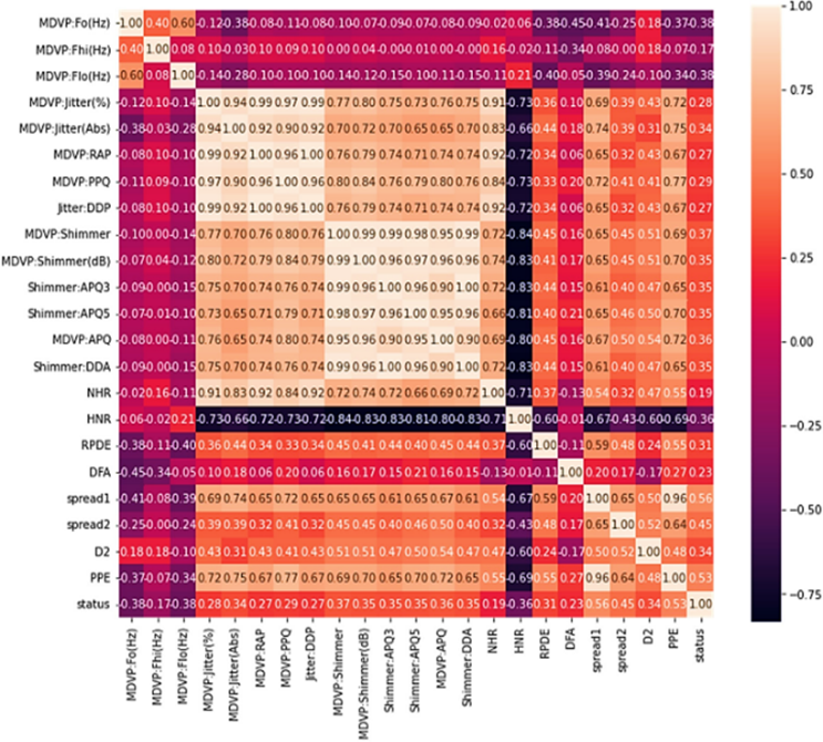
The set of records used in this work is available in the prior section. It has 22 characteristics and includes 195 occurrences in total. The interval between diagnosis and treatment was 0 to 28 years. Every patient had biomedical phonetics information gathered, which might last anywhere from one to thirty-six seconds. An IAC recording equipment and an AKG C420 microphone, placed around 8 cm from the individual's lips, were used to record the audio. These vocal signals were then sent straight to a computer using a CSL 4300B kay. A sample rate of 44.2 kHzs and 16-bit resolution were maintained for every speech transmission. Although amplitude normalisation had an impact on calibration, changes in the mean blood pressure were the main focus of the investigation. The information was structured in ASCII-CSVs, with every column representing a different voice metric and every row corresponding to a patient recording. Each patient provided, on average, around six recordings with different targeted voice metrics. The dataset's initial row contains the names of the patients. Table 2 contains particular details about the database's attributes, while Table 3 contains the statistical evaluation that was done on the collection of data. The current study primarily evaluates classification performance. Although the Android application successfully communicates with the cloud-based diagnostic model, a detailed analysis of processing delay, network latency, and end-to-end response time was outside the scope of this work. Future experimental evaluations will quantify the real-time performance of the system under different network conditions and cloud workloads to ensure suitability for routine clinical use.
Figure 4. Analysis of the dataset's characteristics using a heatmap
Table 3. Database attributes with explanation
|
Name |
Description |
|
ASCII |
Name of Patient with record no. |
|
MDVP-Fos (Hz) |
Voice of average range |
|
MDVP Fhis (Hz) |
Voice of max range |
|
MDVP Flos (Hz) |
Voice of min range |
|
MDVPs jitter (%) |
Various l measurements with various frequency |
|
MDVP Fhis (Hz) |
Various amplitude |
|
NHRs, HNRs |
Ratio of noise for voice |
|
RPDEs, D2s |
Nonlinear factor with complexities |
|
DFAs |
Fractal scales |
|
PPEs, spread1s |
3 non-linear approaches to evaluate the range of variation |
Note: ASCII: American Standard Code for Information Interchange; MDVP: Multi-Dimensional Voice Program; NHR: Noise-to-Harmics Ratio; HNR: Harmonics-to-Noise Ratio; DFA: Detrended Fluctuation Analysis.
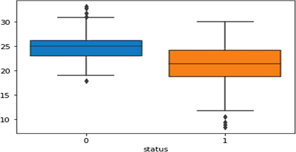
Figure 5. Box plots to evaluate each record's label
Table 4. Evaluation of the dataset's statistics
|
|
Total |
Average |
SD |
Minimum |
50% |
Maximum |
|
MDVP:Fo (Hz) |
195 |
155 |
42.45 |
89 |
150.00 |
261 |
|
MDVP:Fhi (Hz) |
198 |
93.46 |
103 |
178.01 |
560.09 |
|
|
MDVP:Flo (Hz) |
117 |
44.56 |
66 |
105.78 |
234.09 |
|
|
MDVP:Jitter (%) |
0.07 |
0.0049 |
0.0023 |
0.0024 |
0.0234 |
|
|
MDVPs:Jitter (Abs) |
0.00 |
0.0039 |
0.0034 |
0.0024 |
0.345 |
|
|
MDVPs:RAP |
0.003 |
0.0024 |
0.0045 |
0.0034 |
0.432 |
|
|
MDVPs:PPQ |
0.035 |
0.0034 |
0.0018 |
0.0045 |
0.0456 |
|
|
Jitter:DDPs |
0.029 |
0.0034 |
0.0234 |
0.0056 |
0.768 |
|
|
MDVP:Shimmer |
0.043 |
0.0023 |
0.0023 |
0.0034 |
0.0987 |
|
|
MDVP:Shimmer (dB) |
0.046 |
0.0025 |
0.0078 |
0.0045 |
0.967 |
|
|
Shimmer: APQ3s |
0.038 |
0.009 |
0.0045 |
0.0056 |
0.987 |
|
|
Shimmer: APQ5s |
0.38 |
0.001 |
0.0034 |
0.0068 |
0.098 |
|
|
MDVP: APQs |
0.0048 |
0.0076 |
0.0044 |
0.0076 |
0.876 |
|
|
Shimmer: DDAs |
0.0046 |
0.0067 |
0.0045 |
0.0078 |
0.0986 |
|
|
NHRs |
0.033 |
0.0045 |
0.0065 |
0.0087 |
0.0765 |
|
|
HNR |
0.045 |
0.0035 |
0.0056 |
0.0098 |
0.0657 |
|
|
RPDE |
0.056 |
0.0028 |
0.0045 |
0.0067 |
0.0543 |
|
|
DFA |
0.023 |
0.0034 |
0.0036 |
0.0056 |
0.0675 |
|
|
Spread 1 |
0.024 |
0.0345 |
0.0183 |
0.0065 |
0.0876 |
|
|
Spread 2 |
0.035 |
0.0028 |
0.0113 |
0.0047 |
0.0567 |
|
|
D2 |
0.037 |
0.0345 |
0.0123 |
0.0456 |
0.0045 |
|
|
PPE |
0.039 |
0.047 |
0.0012 |
0.654 |
0.0367 |
|
|
Status |
0.032 |
0.045 |
0.0023 |
0.876 |
0.00467 |
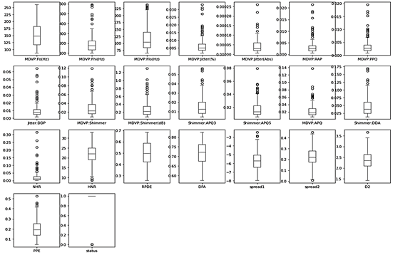
Heatmap analysis is a popular data analysis approach for graphically representing the connections among elements in an analysis. It helps determine which characteristics have strong and weak associations with one another as well as comprehend how these aspects correlate. The vertical and horizontal columns in this illustration reflect the graphical representation of the applied characteristics. Normalised numerical information in the histogram ranges from 0 to 1, with brightness representing 1 and darker colours suggesting 0. Diagonal values are uniformly 1, signifying a complete correlation between features, whereas a decrease in values indicates reduced correlation between features. The distribution of numerical data may be better understood graphically with the use of this tool (Figures 4-6). A box plot is used to show the transportation for every feature's information while evaluating the characteristics in Figure 5. Specifically, Figure 4 illustrates the visualization of the most critical 23 features within the PD dataset under study, as in Table 4. Box plots segment data into sections, each comprising roughly 25% of the database in Figure 6.
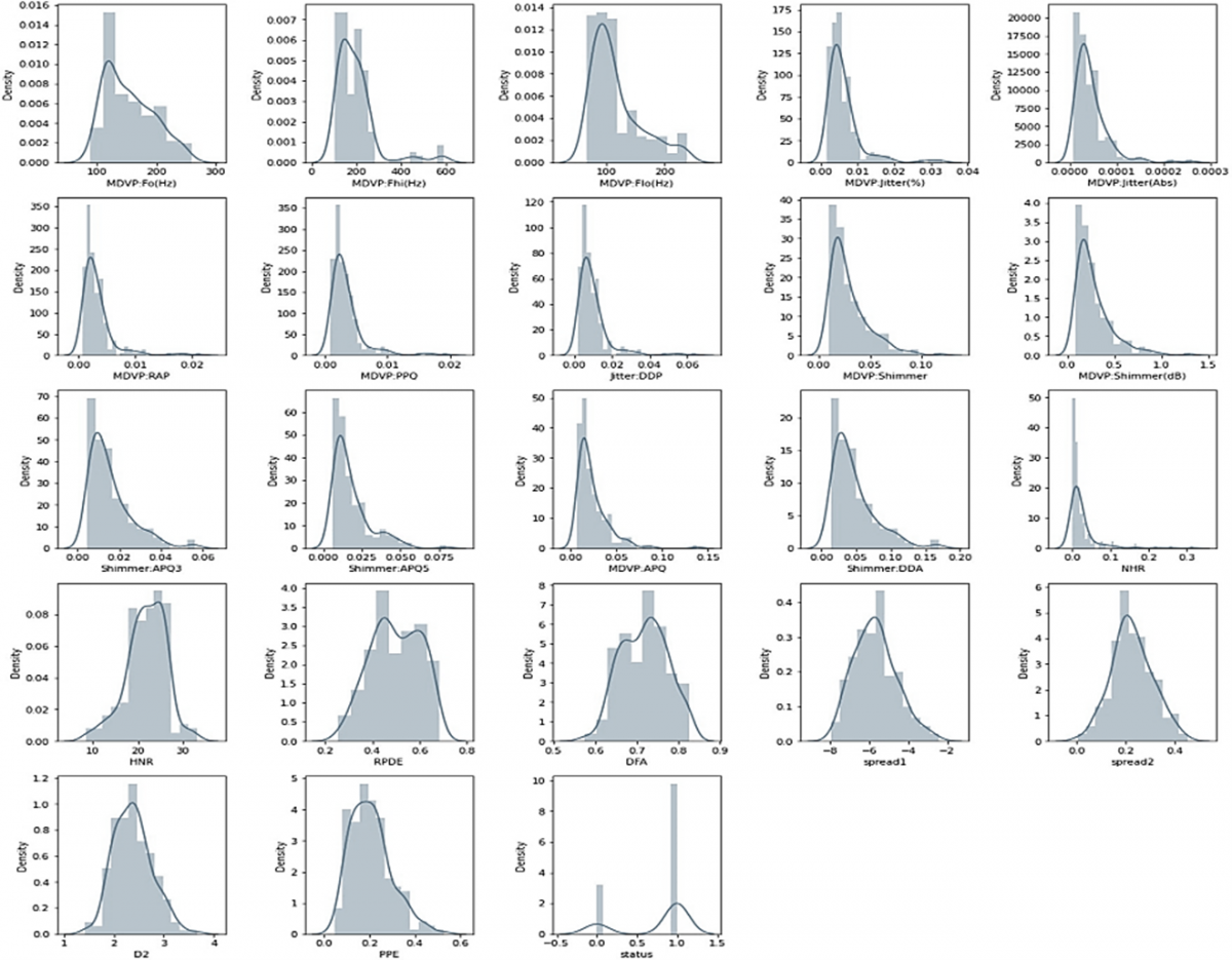
Figure 7 showcases a histogram used for analysing the features within the dataset. This graphical representation depicts the range of information values across various levels, offering a visual insight into the dataset's distribution. Histograms are highly effective tools for visualizing numerical data distribution. Using this common graphing method to capture continuous as well as discrete info that was captured on an interval scale, we analyse the histograms of the attributes in this specific picture. They function as a common way to concisely convey important details of the sharing of data in an understandable style.
Figure 6. A box plot evaluation of the characteristic distributions
Figure 7. Histogram analysis of the characteristic range
One popular tool for analysing information and visualisation using the language of programming, Python, is a Jupyter Notebook. It offers a single framework on which users can easily create and run software, provide visuals, and record discoveries. Running in a web the internet browser, it is compatible with a number of languages, most notably Python 3.8. In order to optimise the hyperparameters of 6 different AI categorization models—the proposed, RF, LR, NB, RC, and DT—this work used MMI FS. Several deep learning methods were used to evaluate the proposed model's efficiency.
$\text{Accuracy}=\frac{\text{TPs}+\text{TNs}}{\text{TPs}+\text{FPs}+\text{FNs}+\text{TNs}}$ (18)
The equation depicted here calculates recall, precision, F1-score.
$\text{Recall}=\text{ }\!\!~\!\!\text{ }\frac{\text{TPs}}{\text{TPs}+\text{FNs}}$ (19)
$\text{Precision}=\text{ }\!\!~\!\!\text{ }\frac{\text{TPs}}{\text{TPs}+\text{FPs}}$ (20)
$\text{F}1-\text{Score}=\text{ }\!\!~\!\!\text{ }\frac{2\text{*Recall*Precision}}{\text{Recall}+\text{Precision}}$ (21)
The experimental phase involved optimizing the hyperparameters for the classification models through MMI.
RF: Utilized 10 estimators, employing the "gini" criterion.
RC: obtained the greatest results with an alpha value of 0.4. "copy_X" was false, "fit_intercept" was true, "normalise" was false, & the "lsqr" solvers were used with a tolerance of 0.01.
DT: Optimal settings involved the "entropy" criterion and the "random" splitter.
NB: Utilized an alpha value of 0.1 and a "var_smoothing" value of 0.00001.
LR: Employed a "l2" penalty and "lbfgs" solver for best performance.
Proposed: Utilized a "rbf" kernel and achieved optimal results with a regularization parameter (C) value set to 0.4.
Table 5. Classification model's parameters utilized
|
Methods |
Best Hyper- Parameter |
|
RF |
N_estimators = 10, criterion = gini. |
|
RC |
Alpha = 0.4, copy_X = false, fit_intercept = true, normalization = false, solver = lsqr, tol = 0.01. |
|
DT |
Criterion = entropies, splitter = randomized |
|
NB |
Alpha = 0.1, var_smoothing = 0.00001. |
|
LR |
Penalties = l2, solved = lbfgs. |
|
Proposed |
Kernel = rbf, Factors of regularization (C) = 0.4. |
Note: RF = Random Forest; RC = Ridge Classifier; DT = Decision Tree; NB = Naïve Bayes; LR = Logistic Regression.
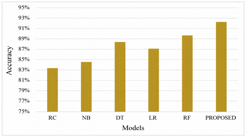
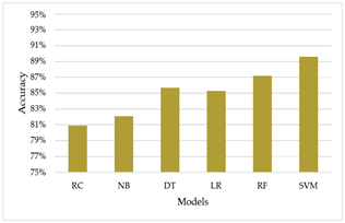
The performance characteristics (precision, F1-score, recall, and accuracy) of every model attained by Probabilistic optimisation are shown in Table 5. With a 94.6% precision, 95.4% F1-score, 94.5% recall, 92.1% accuracy, proposed algorithm that performs the best out of all the models that were evaluated. On the other hand, BO-RC exhibits the worst performance, with 85.5% precision, 85.8% F1-score, 87.36% for recall, 87% accuracy. Additionally, Figure 8 presents an analysis of the categorising algorithms' accuracy utilising the Probabilistic Optimisation approach.
Table 6. Effectiveness of categorising algorithms
|
Methods |
Accuracy (%) |
F1- Measure (%) |
Recall (%) |
Precision (%) |
|
RC |
84.4 |
83.3 |
84.5 |
83.1 |
|
NB |
85.6 |
85.5 |
87.7 |
85.6 |
|
DT |
89.6 |
88.8 |
89.6 |
89.2 |
|
LR |
88.3 |
89.6 |
88.3 |
87.6 |
|
RF |
90.8 |
89.6 |
90.8 |
90.8 |
|
Proposed |
93.4 |
93.6 |
94.3 |
93.5 |
Figure 8. Computing model accuracy
Table 7. Classification of precision models utilising default settings
|
Frame work |
Accuracy (%) |
|
RC |
81.10 |
|
NB |
83.2 |
|
DT |
86.8 |
|
LR |
88.3 |
|
RF |
89.9 |
|
Proposed |
90.8 |
Note: RC = Ridge Classifier; NB = Naïve Bayes; DT = Decision Tree; LR = Logistic Regression; Proposed = proposed random forest–bidirectional long short-term memory–maximized mutual information (RF-BiLSTM-MMI) model; RF = Random Forest; Bi-LSTM = Bidirectional Long Short-Term Memory; MMI = Maximized Mutual Information.
Figure 9. Computing accuracy with default parameter values
Table 6 presents the precision results of the categorization models with default settings. Using standard settings eliminates the requirement for periodic hyperparameter tweaks, which streamlines the modelling process. The scikit-learn library decided these default settings, which are based on industry-accepted best practices and have proven effective in a range of situations. The analysis in Table 7 highlights the proposed model as the most accurate among the models, achieving an accuracy of 89.6%. Following closely, the RF model secures the second position, attaining an accuracy of 88.3%. On the other hand, with a precision of 80.9%, this Ridge Classification algorithm has the worst precision of all the models. Model evaluation was conducted using Leave-One-Out Cross-Validation (LOOCV), which is particularly suitable for small datasets because it maximizes the use of available training samples while reducing estimation bias. Each sample was used once as a testing instance, while all remaining samples were used for training.
The application of MMI for hyperparameter tuning distinctly enhances the models' performance in contrast to their default settings. Through MMI, the optimization of hyperparameters notably enhances the accuracy across all approaches. Figure 9 compares the classification of precision models using normal hyperparameters.
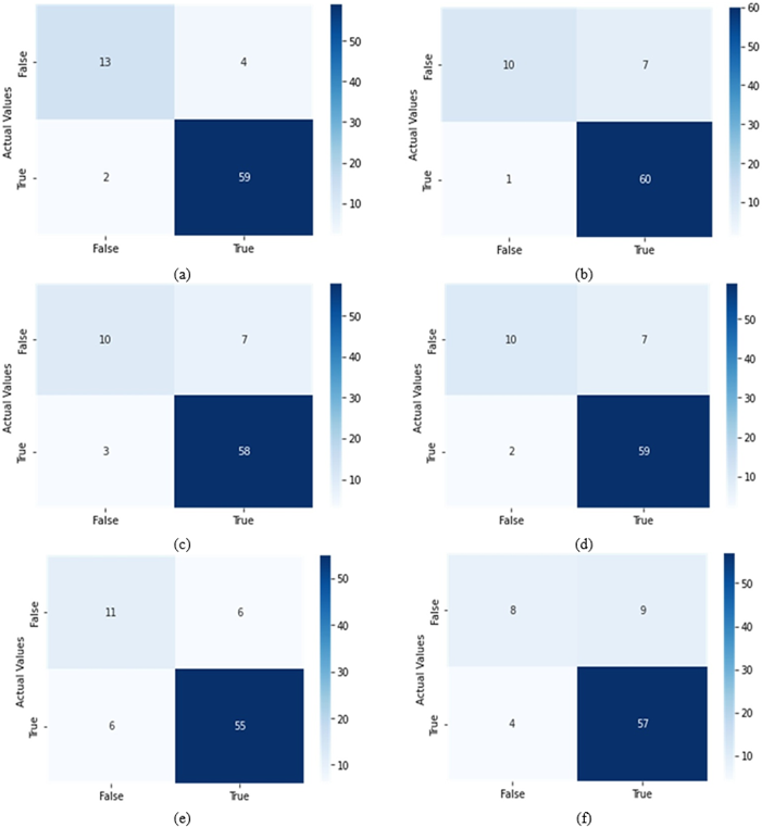
The study's outcomes underwent additional assessment through confusion matrices, visually depicted in Figure 10. These matrices offered a more comprehensive evaluation of each classifier's performance. The analysis revealed that BO-proposed showcased superior performance compared to the other classifiers.
4.1 Discussion
This paper presents an innovative approach to differentiate between individuals affected by PD and those who are not. Employing MMI, the study tunes hyperparameters for 6 various ML models: proposed RF-BiLSTM-MMI, RF, LR, NB, RC, and DT. The dataset comprises 23 features and 195 instances, and the models’ performances are assessed using precision, F1-measure, recall, and accuracy. The proposed model outperforms others both pre- and post-hyperparameter tuning, achieving 93.4% accuracy through MMI. This research contributes significantly to machine learning applications in healthcare. The study [31] utilized a Bi-LSTM neural network and proposed classification to diagnose speech deficits in early-stage central nervous system illnesses. Utilising 339 speech samples from 15 people, their technique obtained 95.50% (BiLSTM) and 96.4% (Proposed) reliability for classifying persons as either fit or deficient. Interpretability remains an important consideration for clinical adoption. The selected voice biomarkers correspond to known speech abnormalities observed in PD. Increased jitter and shimmer values indicate impaired neuromuscular control of vocal fold vibration, while reduced HNR reflects vocal roughness and breathiness. These physiological manifestations are directly associated with motor impairments caused by dopaminergic neuron degeneration. Consequently, the selected features provide a biologically meaningful representation of Parkinsonian speech characteristics despite the complexity of the machine learning model.
Regarding the choice of MMI for hyperparameter optimization among several other tools, MMI holds distinct advantages:
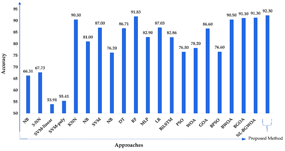
The validation set, sometimes referred to as the test set, is created using the leave-one-out cross-validation technique by taking one observation out of the original dataset, and the training set is created utilising the extra observations. Using a single finding as validation information, the procedure is repeated N times. Using the suggested approach, the classifier's performance is evaluated on hypothetical cases. The proportion of accurate classifications obtained throughout the course of N repetitions is used to evaluate performance. The test subject is removed from the initial database before the set of training data is created in order to guarantee that the characteristics of the data used for training, and hence the learned classifier, are unaffected by the validation sample. Obtaining the required subject scores for the classifier's activation is done in this stage. The classifier then decides what the test subject's label is [29]. We carried out a comparative analysis by making use of the standard dataset that was retrieved from the University repository. The comparison of our suggested method with the methods that were stated is depicted in Figure 11, which uses the same applicable PD standard database as the other methods. Dataset size remains one of the primary limitations of the present study. The PD voice dataset contains 195 recordings collected from only 32 subjects, including 24 PD patients and 8 healthy controls. Although the dataset is widely used as a benchmark for PD classification research, the relatively small sample size and class imbalance may affect the generalizability of the developed model. To mitigate this limitation, feature selection using MMI and hyperparameter optimization were employed to reduce overfitting and improve model robustness. Future work will involve validation on larger multi-center datasets containing participants from different demographic and clinical backgrounds. Although the proposed RF-BiLSTM-MMI framework achieved encouraging classification performance, clinical validation against established diagnostic instruments such as the Unified Parkinson's Disease Rating Scale (UPDRS) and Movement Disorder Society-UPDRS was not performed in the current study. The observed performance improvement of the proposed RF-BiLSTM-MMI framework over conventional classifiers suggests that the integration of feature selection and hybrid learning contributes positively to classification performance. Future studies will incorporate statistical significance testing, such as paired t-tests or McNemar's tests, to further validate the superiority of the proposed approach. To further improve model transparency and clinical trust, future work will investigate explainable AI techniques such as SHAP and LIME. These approaches can quantify feature contributions and provide interpretable explanations for individual predictions generated by the proposed framework.
Figure 11. Comparing the suggested model with current methods that make use of the same common Parkinson's disease (PD) database
Therefore, the reported accuracy should be interpreted as a machine-learning evaluation rather than a replacement for clinical diagnosis. Future studies will focus on validating the proposed framework using clinically annotated patient cohorts and comparing predictions against neurologist assessments and UPDRS scores.
4.2 Ethical and privacy considerations
The proposed cloud-based diagnostic framework processes sensitive voice recordings that may contain identifiable patient information. Therefore, data privacy and security are critical considerations. During cloud transmission, patient information should be protected using secure communication protocols such as HTTPS and TLS encryption. Furthermore, stored data should be anonymized and access-controlled in compliance with applicable healthcare regulations, including HIPAA and GDPR guidelines. The current implementation focuses on technical feasibility, while future deployments will incorporate comprehensive privacy-preserving mechanisms and regulatory compliance procedures.
4.3 Study limitations
Despite the encouraging performance of the proposed framework, several limitations should be acknowledged. First, the study utilized a relatively small dataset consisting of 195 voice recordings obtained from only 32 subjects, which may limit the generalizability of the findings. Second, the dataset exhibits class imbalance, with substantially more PD recordings than healthy controls. Third, external validation using independent datasets was not performed. Finally, clinical parameters such as disease severity, UPDRS scores, medication status, and longitudinal follow-up information were unavailable. Future studies will address these limitations through larger multicenter datasets and prospective clinical validation.
This article employs machine learning (ML) techniques to build a cloud-based PD diagnosis system, focusing on feature selection and classification. The development of the diagnosis model involves using a combination of Bi-LSTM and RF classification algorithms. Furthermore, the MMI selection algorithm is incorporated to decrease the overall number of features used in the process. The diagnosis model is made available to users by means of an Android mobile application that features a user-friendly interface for testing PD. This application is deployed on the Google Cloud Application Engine. 195 cases are included in the dataset that was used, and there are 23 features. The binary value of the target feature shows that there is PD when it is 1 and that there is no PD when it is 0. SVM, RF, LR, NB, Ridge Classifier, and DT are shown before and after adjusting hyperparameters through BO. Following tuning, the proposed RF-BiLSTM-MMI framework achieved the best performance among all evaluated models, attaining an accuracy of 93.4%, an F1-score of 93.6%, a recall of 94.3%, and a precision of 93.5%. The results confirm that combining MMI feature selection with hybrid machine learning and deep learning classifiers can effectively identify PD from voice recordings. The cloud-based deployment architecture further enables practical implementation through mobile healthcare applications and remote patient screening systems.
The dataset might be expanded in the future to encompass a more diverse and representative sample. Exploring advanced machine learning techniques like deep learning could potentially yield enhanced results. Experimentation with various feature selection methods is recommended. Additionally, validating the outcomes on an independent dataset could bolster confidence in the proposed model's robustness and predictability.The current framework focuses on cross-sectional classification of PD using individual voice recordings. Longitudinal monitoring of disease progression was not investigated. Future research will explore repeated voice assessments collected over extended periods to determine the ability of the proposed framework to track disease progression, treatment response, and symptom evolution.
It is possible that the future course of the study will involve generalisation across a wider range of people, with the possibility of incorporating it into a more comprehensive healthcare system by utilising fog computing and the Internet of Medical Things.
[1] Govindu, A., Palwe, S. (2023). Early detection of Parkinson's disease using machine learning. Procedia Computer Science, 218: 249-261. https://doi.org/10.1016/j.procs.2023.01.007
[2] Belić, M., Bobić, V., Badža, M., et al. (2019). Artificial intelligence for assisting diagnostics and assessment of Parkinson’s disease-A review. Clinical Neurology and Neurosurgery, 184: 105442. https://doi.org/10.1016/j.clineuro.2019.105442
[3] Palanisamy, P., Urooj, S., Arunachalam, R., Lay-Ekuakille, A. (2023). A novel prognostic model using chaotic CNN with hybridized spoofing for enhancing diagnostic accuracy in epileptic seizure prediction. Diagnostics, 13(21): 3382. https://doi.org/10.3390/diagnostics13213382
[4] Preethi, P., Asokan, R. (2019). A high secure medical image storing and sharing in cloud environment using hex code cryptography method—Secure genius. Journal of Medical Imaging and Health Informatics, 9(7): 1337-1345. https://doi.org/10.1166/jmihi.2019.2757
[5] LN, P. (2023). Transfer driven ensemble learning approach using ROI pooling CNN for enhanced breast cancer diagnosis. Journal of Machine and Computing, 297-311.
[6] Palanisamy, P., Padmanabhan, A., Ramasamy, A., Subramaniam, S. (2023). Remote patient activity monitoring system by integrating IoT sensors and artificial intelligence techniques. Sensors, 23(13): 5869. https://doi.org/10.3390/s23135869
[7] Pramanik, M., Pradhan, R., Nandy, P., Qaisar, S.M., Bhoi, A.K. (2021). Assessment of acoustic features and machine learning for Parkinson’s disease detection. Journal of Healthcare Engineering, 2021: 9957132. https://doi.org/10.1155/2021/9957132
[8] Meral, M., Ozbilgin, F., Durmus, F. (2025). Fine-tuned machine learning classifiers for diagnosing Parkinson’s disease from vocal characteristics: A comparative analysis. Diagnostics, 15(5): 645. https://doi.org/10.3390/diagnostics15050645
[9] Cantürk, İ., Karabiber, F. (2016). A machine learning system for the diagnosis of Parkinson’s disease from speech signals and its application to multiple speech signal types. Arabian Journal for Science and Engineering, 41: 5049-5059. https://doi.org/10.1007/s13369-016-2206-3
[10] Painuli, D., Bhardwaj, S., Kose, U. (2025). Efficient feature selection and hyperparameter tuning for improved speech signal-based Parkinson’s disease diagnosis via machine learning techniques. Health Technology Assessment and Action, 9(1): 26-41. https://doi.org/10.18502/htaa.v9i1.17863
[11] Alshammri, R., Alharbi, G., Alharbi, E., Almubark, I. (2023). Machine learning approaches to identify Parkinson’s disease using voice signal features. Frontiers in Artificial Intelligence, 6: 1084001. https://doi.org/10.3389/frai.2023.1084001
[12] Tekindor, A.N., Aydın, E.A. (2024). Feature selection improves speech based Parkinson’s disease detection performance. In Proceedings of the 17th International Joint Conference on Biomedical Engineering Systems and Technologies - Volume 1: BIOSIGNALS, pp. 726-732. https://doi.org/10.5220/0012347300003657
[13] Rana, A., Dumka, A., Singh, R., Rashid, M., Ahmad, N., Panda, M.K. (2022). An efficient machine learning approach for diagnosing Parkinson’s disease by utilizing voice features. Electronics, 11(22): 3782. https://doi.org/10.3390/electronics11223782
[14] Dao, S.V., Yu, Z., Tran, L.V., et al. (2022). An analysis of vocal features for Parkinson’s disease classification using evolutionary algorithms. Diagnostics, 12(8): 1980.
[15] Gunduz, H. (2025). Efficient Parkinson’s disease classification from speech with filter-based feature selection and Genetic Algorithm–Bayesian Optimization ensemble integration. PeerJ Computer Science, 11: e3430. https://doi.org/10.7717/peerj-cs.3430
[16] Pamulaparthyvenkata, S., Sharma, J., Dattangire, R., et al. (2024). Deep learning and EHR-driven image processing framework for lung infection detection in healthcare applications. In 2024 15th International Conference on Computing Communication and Networking Technologies (ICCCNT), pp. 1-7. https://doi.org/10.1109/ICCCNT61001.2024.10724177
[17] Lamba, R., Gulati, T., Jain, A. (2022). A hybrid feature selection approach for Parkinson’s detection based on mutual information gain and recursive feature elimination. Arabian Journal for Science and Engineering, 47: 10263-10276. https://doi.org/10.1007/s13369-021-06544-0
[18] Qadir, J.A. (2025). Enhancing Parkinson’s disease detection by combining SMOTE and feature selection for improved machine learning classification using voice recordings. Journal of Voice. https://doi.org/10.1016/j.jvoice.2025.11.003
[19] Xu, H.Q., Xie, W., Pang, M.Z., et al. (2025). Non-invasive detection of Parkinson’s disease based on speech analysis and interpretable machine learning. Frontiers in Aging Neuroscience, 17: 1586273. https://doi.org/10.3389/fnagi.2025.1586273
[20] Al-Nefaie, A.H., Aldhyani, T.H.H., Kounda, D. (2024). Developing system-based voice features for detecting Parkinson’s disease using machine learning algorithms. Journal of Disability Research, 3(1): e20240001. https://doi.org/10.57197/JDR-2024-0001
[21] Bhuvaneswari, T., Selvi, M.C., Priyadarsini, R.N., Eswaran, U., Babu, R.R. (2022). Feature selection with mutual information based cuckoo search optimization for Parkinson’s disease prediction. NeuroQuantology, 20(10): 1296-1306. https://doi.org/10.14704/nq.2022.20.10.NQ55099
[22] Sultani, Z.N., Yousif, S.A. (2018). Hybrid feature selection based on mutual information and AUC for Parkinson’s disease classification. Journal of Theoretical and Applied Information Technology, 96(18): 6053-6063.
[23] Devarajan, M., Ravi, L. (2019). Intelligent cyber-physical system for an efficient detection of Parkinson disease using fog computing. Multimedia Tools and Applications, 78: 32695-32719. https://doi.org/10.1007/s11042-018-6898-0
[24] Malekroodi, H.S., Lee, B.I., Yi, M. (2025). Voice-based detection of Parkinson’s disease using machine learning and deep learning approaches: A systematic review. Bioengineering, 12(11): 1279. https://doi.org/10.3390/bioengineering12111279
[25] Pathak, P., Akashe, S., Upadhyay, G.M. (2025). Early detection of Parkinson’s disease through supervised machine learning techniques on voice data. Informatics in Medicine Unlocked, 59: 101705. https://doi.org/10.1016/j.imu.2025.101705
[26] Shinde, S., Satav, S., Shirole, U., Oak, S. (2022). Comprehensive analysis of Parkinson disease prediction using vocal parameters. In 2022 International Conference on Machine Learning, Big Data, Cloud and Parallel Computing (COM-IT-CON), Faridabad, India, pp. 369-373. https://doi.org/10.1109/COM-IT-CON54601.2022.9850857
[27] Steena, T.B., Perumal, P., Suganthi, C., Asokan, R., Sreeji, S., Preethi, P. (2022). Optimizing image fusion using wavelet transform based alternative direction multiplier method. In 2022 2nd International Conference on Advance Computing and Innovative Technologies in Engineering (ICACITE), pp. 2021-2024. https://doi.org/10.1109/ICACITE53722.2022.9823804
[28] Yang, Z.X., Zhou, H., Srivastav, S., et al. (2025). Optimizing Parkinson’s disease prediction: A comparative analysis of data aggregation methods using multiple voice recordings via an automated artificial intelligence pipeline. Data, 10(1): 4. https://doi.org/10.3390/data10010004
[29] Khan, M., Moiz, A., Khan, G.N., Wajid, M., Usman, M., Ali, J. (2025). An FPGA prototype for Parkinson’s disease detection using machine learning on voice signal. IEEE Access, 13: 91113-91128. https://doi.org/10.1109/ACCESS.2025.3572092.
[30] Al Mamun, K.A., Alhussein, M., Sailunaz, K., Islam, M.S. (2017). Cloud based framework for Parkinson’s disease diagnosis and monitoring system for remote healthcare applications. Future Generation Computer Systems, 66: 36-47. https://doi.org/10.1016/j.future.2015.11.010
[31] Carrón, J., Campos-Roca, Y., Madruga, M., Pérez, C.J. (2021). A mobile-assisted voice condition analysis system for Parkinson’s disease: Assessment of usability conditions. BioMedical Engineering OnLine, 20: 114. https://doi.org/10.1186/s12938-021-00951-y
[32] Sajal, M.S.R., Ehsan, M.T., Vaidyanathan, R., Wang, S., Aziz, T., Al Mamun, K.A. (2020). Telemonitoring Parkinson’s disease using machine learning by combining tremor and voice analysis. Brain Informatics, 7: 12. https://doi.org/10.1186/s40708-020-00113-1
[33] Ullah, M.T., Shefa, S.H., Rafid, S.T.S., et al. (2026). An intelligent AI framework for Early Parkinson's Disease Diagnosis Using PCA-Enhanced Vocal Feature Engineering. In 2026 IEEE 2nd International Conference on Quantum Photonics, Artificial Intelligence & Networking (QPAIN), pp. 1-6. https://doi.org/10.1109/QPAIN69676.2026.11546635
[34] Islam, M.S., Adnan, T., Abdelkader, A., et al. (2025). Remote AI screening for parkinson’s disease: A multimodal, cross-setting validation study. Research Square, rs-3. https://doi.org/10.21203/rs.3.rs-6844936/v1
[35] Bai, D.P., Preethi, P. (2016). Security enhancement of health information exchange based on cloud computing system. International Journal of Scientific Engineering and Research, 4(10): 79-82.