Srilakshmi Ravali Madabhushanam* | Mohamed Mansoor Roomi Sindha
© 2026 The authors. This article is published by IIETA and is licensed under the CC BY 4.0 license (http://creativecommons.org/licenses/by/4.0/).
OPEN ACCESS
Reliable identification of a bus's motion state is essential for interpreting passenger boarding and alighting activities from surveillance videos, as these activities should occur only when the bus is stationary. Automatically determining whether a bus is MOVING or STILL from exterior-mounted Closed-Circuit Television (CCTV) videos is challenging because passenger movement near the entrance generates strong optical-flow patterns that often obscure the true vehicle motion. To address this problem, this paper proposes Bus Dynamic Stream, a background-isolated temporal motion learning framework for classifying bus motion states as MOVING or STILL. Rather than analysing the complete optical-flow field, motion features are extracted only from carefully selected background regions to minimize interference caused by passenger movements. This enables the extracted motion information to more accurately represent the actual vehicle dynamics. An 18-dimensional motion representation capturing vehicle translation, vibration, and temporal motion characteristics is constructed from the isolated background flow. The temporal feature sequence is then learned using a Multi-Scale Residual CNN-BiGRU-Attention network for binary bus motion-state classification. Experiments conducted on a real-world dataset comprising 400 bus videos achieved an overall accuracy of 89.98%, a macro F1-score of 0.893, and an Area Under the Curve–Receiver Operating Characteristic (AUC-ROC) of 0.9001. Video-level evaluation using majority voting achieved an accuracy of 91.60%, confirming the temporal consistency of the proposed framework. The results demonstrate that the proposed background isolation effectively reduces passenger-induced motion interference and improves the reliability of bus motion-state classification under crowded boarding and alighting conditions.
bus motion-state classification, optical flow, background motion isolation, temporal representation learning, video surveillance, intelligent transportation systems
Public transportation systems, particularly city buses, operate under highly dynamic and unconstrained environments where passenger safety remains a major concern.
Among various safety-critical situations, activities occurring near the footboard region, such as boarding, alighting, and standing close to the entrance, require continuous monitoring. In many intelligent transportation systems, automatic analysis of passenger behavior is becoming increasingly important for preventing accidents and improving operational safety. A fundamental observation is that the interpretation of passenger behavior strongly depends on the motion state of the bus. For example, a passenger standing on the footboard while the bus is stationary may represent a normal boarding activity. However, the same behavior becomes potentially dangerous when the bus is moving. Activities such as leaning outside of the bus, running alongside the bus, and standing near the entrance can have varying safety implications depending on whether the bus is moving or stationary. Hence, reliable bus motion-state classification forms an important prerequisite for higher-level passenger safety assessment systems. Though bus motion-state classification using onboard CCTV in computer vision and intelligent transportation systems has been extensively studied, the motion estimation of a bus based on onboard CCTV video is a challenging problem. Exterior-mounted surveillance cameras capture a complex combination of sources of motion such as vehicle ego-motion, passenger movements near the footboard, camera vibration and motion from the surrounding environment. When the vehicle has crowded boarding situations, passenger activity often generates strong local optical-flow patterns that may dominate the motion field. This makes it difficult to identify the motion of the vehicle and the movement of the passengers and making the separation of the two very difficult, particularly when the bus is moving slowly or approaching a stop.
One of the important problems in computer vision that has attracted researchers' attention for a long time is understanding motion from video sequences. Optical flow is one of the widely used methods of motion estimation, as it captures how a pixel moves between two consecutive frames. Optical flow is a field with a long history of application in classical optical flow methods like Horn–Schunck and Lucas–Kanade, which have been widely employed in surveillance, object tracking and autonomous navigation [1, 2].
Dense optical flow methods are particularly useful in dynamic environments because they provide motion information for all pixels in the image rather than sparse feature points. Visual odometry is an alternative method to estimate camera motion using feature matching or geometric transformations between frames [3]. These methods have demonstrated strong performance in robotics and autonomous driving applications where camera calibration and structured environments are available. However, their computational complexity and dependence on accurate feature matching may limit their suitability for real-time deployment in crowded and unconstrained public transportation environments.
Another important area of research in surveillance is the analysis of motion in videos acquired using moving cameras. In such scenarios, the observed motion consists of both camera-induced motion and independently moving objects. Existing approaches address this challenge through ego-motion estimation, motion segmentation, and background–foreground separation techniques [4]. Although these methods improve motion interpretation, many rely on geometric modelling, scene assumptions, or optimization procedures that can be computationally demanding for practical edge-based systems.
By combining enhanced instance segmentation, Kalman filtering, spatiotemporal graph convolution, and wavelet-based temporal analysis, Liang presented a video image processing framework for classroom interaction detection. The suggested approach maintained real-time performance while successfully quantifying classroom interactions. The framework's reliance on stable object tracking restricts its application to highly dynamic transit situations, where ego-motion and fast passenger movement are widespread, even though it successfully models human interactions in indoor educational settings [5].
Temporal modelling techniques based on deep learning have also attracted significant attention in recent years. For temporal activity recognition, hybrid deep learning architectures that integrate sequential and convolutional models have also demonstrated encouraging results. For Distributed Acoustic Sensing (DAS) signals, Rajarathinam et al. created a CNN-BiLSTM system in which BiLSTM records long-term temporal dependencies and convolutional layers extract local spatial patterns [6]. In addition, hybrid CNN–RNN architectures have demonstrated promising performance in action recognition and video understanding tasks by jointly learning spatial and temporal representations. However, most existing studies focus on motion segmentation, human activity recognition, or object tracking rather than the estimation of vehicle motion states in the presence of passenger-induced motion interference. These approaches are capable of learning temporal dependencies more effectively than conventional frame-based methods.
Furthermore, in intelligent transportation systems, significant research has focused on vehicle perception, object detection, traffic scene understanding, and vehicle tracking. Comparatively fewer works address bus-mounted surveillance systems, particularly exterior CCTV-based monitoring near the footboard region. Accurate motion estimation in real-world bus environments is challenging due to passenger movement, occlusions, varying crowd density, and vehicle-induced vibrations. As a result, conventional optical flow magnitude thresholding often produces unreliable estimates because passenger movements dominate the motion field even when the bus is stationary. The existing methods do not explicitly isolate stable background motion regions to suppress passenger-induced disturbances during feature extraction. As a result, their performance significantly degrades during crowded boarding and low-speed movement scenarios.
Temporal representation learning has evolved from hand-crafted descriptors such as HOG, HOF, and dense trajectories [7, 8] to deep learning-based approaches including Two-Stream Networks, I3D, and recurrent architectures such as LSTM and GRU [9, 10]. These methods effectively capture spatiotemporal patterns in generic action recognition tasks using RGB frames and optical flow. The study proposed an attention-guided residual network for low-light image enhancement, which decomposes the image, adds multi-scale attention and residual learning, and enhances the visibility and noise suppression of the image. These methods are preprocessing methods that enhance the quality of images and feature extraction but do not explicitly model the time-related motion information, which is needed in activity recognition [11]. However, conventional video representations are primarily designed for appearance-driven action analysis and are less suited for modelling long-duration vehicular dynamics such as vibration, inertia variation, and jerk patterns.
Motion disentanglement aims to separate ego-motion from independently moving scene objects. Classical geometry-based approaches relied on epipolar constraints, homography estimation, and RANSAC-based motion modelling [12], while deep learning methods improved dense optical flow estimation. Recent self-supervised frameworks further integrated depth and ego-motion estimation for scene decomposition. However, existing methods do not explicitly address persistent passenger-motion contamination in crowded bus interiors, where foreground motion occupies a large portion of the visual field.
Weak ego-motion estimation aims to infer platform motion directly from visual cues without relying on external sensors such as IMUs or GPS. Traditional visual odometry and SLAM-based approaches, including ORB-SLAM [13], SfM-Net estimates the relative camera motion between video frames while simultaneously modelling scene structure and independently moving objects [14], while self-supervised frameworks jointly learn depth and pose estimation from monocular video sequences [3, 15]. In lightweight vehicular sensing applications, simplified motion descriptors derived from optical flow have also been explored for ride quality and road condition analysis.
Dynamic scene segmentation methods traditionally rely on background subtraction techniques. Although effective in static-camera scenarios, their performance degrades under camera motion. Deep semantic segmentation approaches, including DeepLab and panoptic segmentation frameworks, improve foreground-background separation through semantic understanding [16, 17]. In bus interior environments, dynamic segmentation is essential for isolating structural background regions from passenger motion.
Camera motion significantly affects conventional action recognition systems because ego-motion can distort motion-based discriminative features and reduce foreground-background consistency. Transformer architecture based multi-head self-attention mechanism allows relationships among different video representations and activity recognition [18]. Existing approaches mitigate these effects through camera-motion compensation, trajectory stabilization, and temporally distributed frame sampling strategies, as demonstrated by Improved Dense Trajectories and Temporal Segment Networks (TSN). Recent deep learning frameworks, including Two-Stream Networks and I3D, further improve the extraction of spatiotemporal representations from video sequences under dynamic viewing conditions.
Transformer-based video models [19] and ConvLSTM [20] architectures have demonstrated strong performance in large-scale video understanding tasks by learning long-range temporal dependencies. However, these approaches generally require large training datasets and higher computational resources. Since the present work focuses on optical-flow-based temporal motion learning using a comparatively smaller dataset, a lightweight CNN-BiGRU framework is adopted for efficient bus motion-state classification.
From the above studies, three observations can be made. First, existing methods mainly estimate vehicle motion directly from optical flow or visual odometry. Second, several studies attempt to separate camera motion from foreground motion, but they do not specifically address passenger movement in bus surveillance videos. Third, CNN-RNN models effectively learn temporal information when reliable motion features are available [21, 22]. These observations motivate the proposed framework, where background motion is first isolated and then learned using a temporal deep learning model for bus motion-state classification.
From the isolated background regions, a compact set of eighteen optical-flow-based descriptors is extracted. These descriptors capture multiple aspects of bus dynamics, including ego-motion, vibration, inter-frame displacement, acceleration, jerk, motion coherence, directional consistency, spatial asymmetry, flow-distribution statistics, and higher-order temporal characteristics. Collectively, these studies demonstrate the effectiveness of deep learning, attention mechanisms, graph neural networks, and hybrid CNN-recurrent architectures for visual understanding tasks. However, most existing approaches are designed for relatively stable environments, depend on accurate pose estimation or object tracking, or primarily improve image quality rather than motion representation. Few methods explicitly address challenging transportation scenarios characterized by significant camera ego-motion, passenger occlusions, and complex boarding behaviours. These limitations motivate the development of more robust spatiotemporal [21] frameworks capable of effectively recognizing passenger activities in real-world bus environments. The resulting feature sequence is then processed using a Multi-Scale Residual CNN–BiGRU–Attention architecture. The multi-scale convolutional layers learn short-term temporal variations occurring at different motion scales, while the BiGRU captures long-range temporal dependencies. A temporal attention mechanism further emphasizes the most informative motion segments for classification.
The main contributions of this work are summarized as follows:
•A background-region-based motion isolation strategy that suppresses passenger-induced motion interference and improves the reliability of vehicle motion estimation.
•A comprehensive motion representation consisting of eighteen optical-flow-based descriptors capturing ego-motion, vibration, acceleration, jerk, motion coherence, directional consistency, spatial asymmetry, and flow-distribution characteristics.
•A Multi-Scale Residual CNN–BiGRU–Attention architecture that jointly learns short-term motion variations and long-range temporal dependencies for robust bus-state classification.
•A comprehensive evaluation is conducted with real-world bus surveillance videos, demonstrating reliable performance under challenging conditions involving crowding, vibration, and slow-moving speeds.
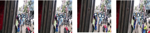
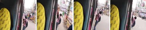
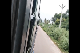
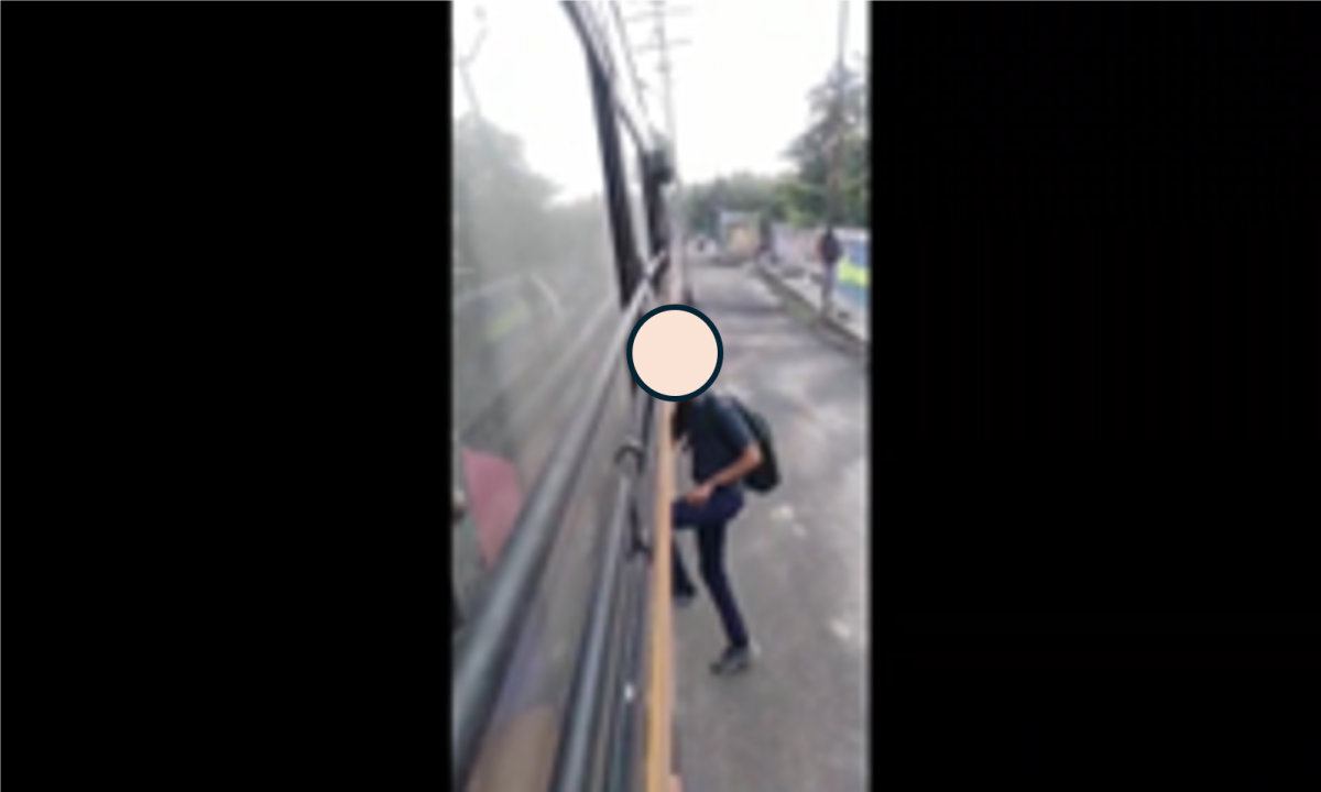
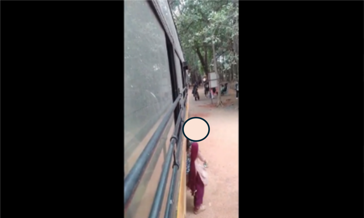
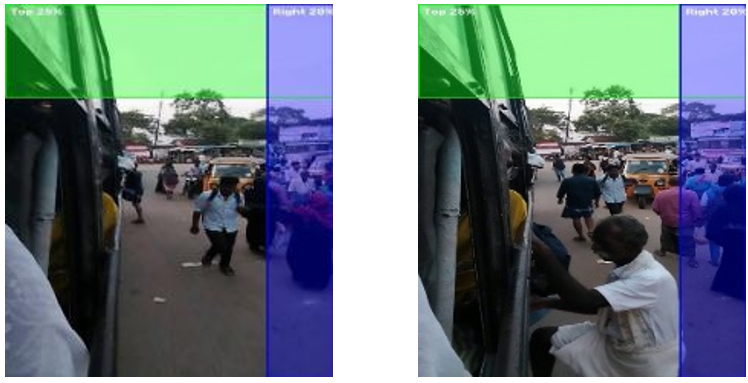
The dataset was collected using exterior-mounted CCTV cameras installed near the bus footboard region. The recordings capture both passenger activity and surrounding background structures under real operating conditions. A representative sample of frames from the acquired dataset has been shown in Figure 1.
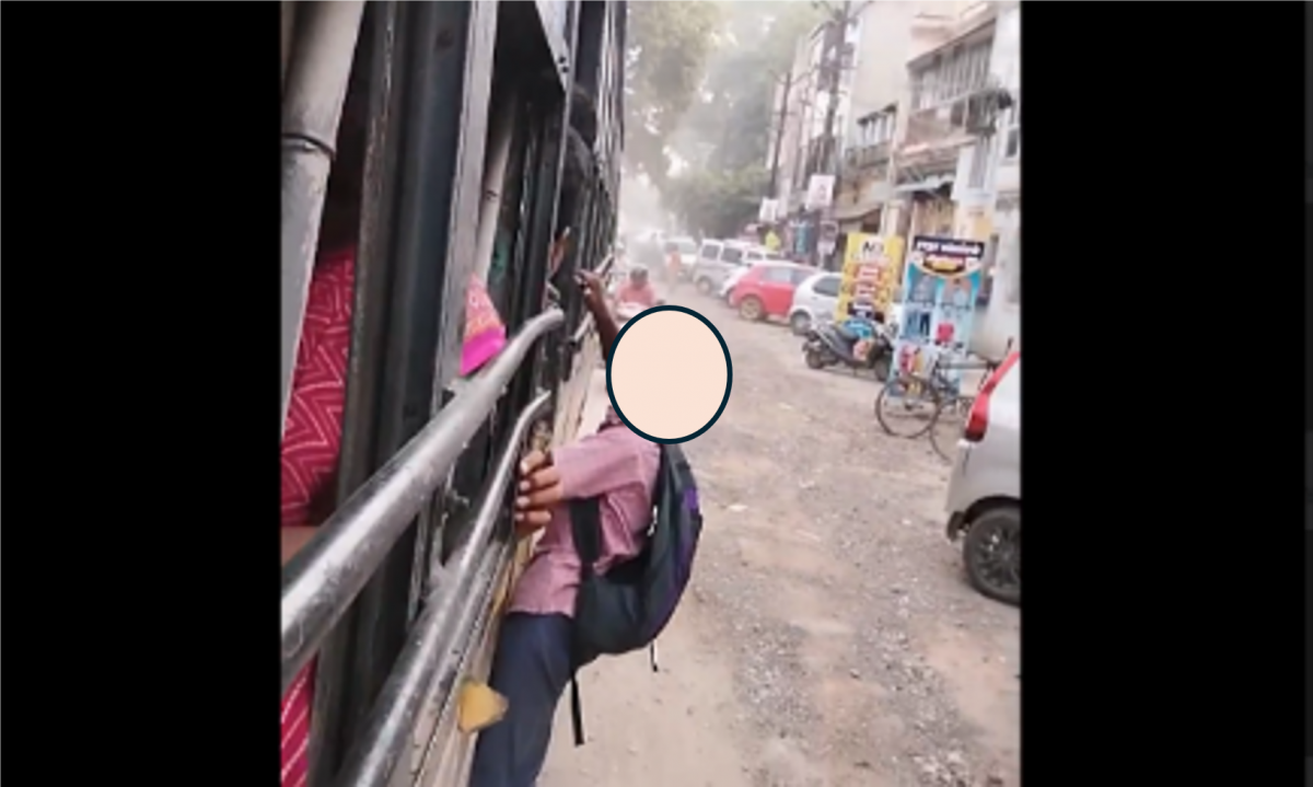
The dataset comprises video clips captured during different passenger activities commonly observed in public transportation environments, such as Safe Journey (SJ), Foot Boarding (FB), Bus Boarding (BB), and Getting Down (GD) scenarios. A total of 100 videos were recorded for each activity category, resulting in a dataset of 400 labelled video sequences. The number of videos collected per bus ranged from 2 to 10, depending on the availability of the corresponding passenger activities. These activity categories were grouped into two motion-state classes, namely STILL and MOVING. The final balanced dataset consists of 200 videos for each motion class, ensuring a balanced distribution to train and test the models. The videos were labelled at the level of the individual frames, and representative key frames were extracted and further classified at the action level, including safe boarding, unsafe boarding, safe alighting, unsafe alighting, and foot boarding, as shown in Figure 2. These samples show diverse passenger postures, movement directions, and interactions near the bus entrance, which are important for analysing real-world passenger behaviour.
Data were collected under different lighting conditions, crowd densities, vehicle speeds, and environmental conditions to enhance robustness and generalization. The dataset thus has both stationary and moving bus scenarios, and significant variation in the level of passenger activity, which allows the proposed framework to learn discriminative motion patterns under realistic operating conditions. These variations make the evaluation more representative of real-world deployment scenarios. Among the 400 video sequences, 280 were used for training, 60 for validation, and 60 for testing. Table 1 summarizes the dataset structure. Depending on the video, we receive sequences from 2.4 seconds to 20.1 seconds of video at 30 fps (mean 7 seconds).
Table 1. Dataset summary
|
Split |
Total |
STILL |
MOVING |
|
Train |
280 |
140 |
140 |
|
Validation |
60 |
30 |
30 |
|
Test |
60 |
30 |
30 |
|
Total |
400 |
200 |
200 |
Our test dataset comprises a total of 30 videos per class, which have never been seen during training and hyperparameter selection. Table 2 shows the class labels and the distribution of the dataset for further processing.
Table 2. Training and test dataset distribution
|
Folder |
Class |
Label |
Videos |
|
BB_Train |
STILL |
0 |
70 |
|
GD_Train |
STILL |
0 |
70 |
|
FB_Train |
MOVING |
1 |
70 |
|
SJ_Train |
MOVING |
1 |
70 |
|
Test Set |
Both |
0/1 |
60 |
Note: BB = Bus Boarding; GD = Getting Down; FB = Foot Boarding; SJ = Safe Journey.
Dataset Split Policy and Data Integrity: To make sure the evaluation is fair and there is no data leakage between training and testing, the dataset was divided based on the bus from which the videos were collected. Videos from the same bus were kept only in one dataset, either training, validation, or testing. So, the same bus was not used in more than one set. Also, all the frames from one video were kept together in the same set to avoid frame-level data leakage. The dataset represents different real-world situations that can occur inside buses, such as partial occlusion, different numbers of passengers, and background noise. The videos were collected from 50 different buses running on urban and semi-urban routes. Videos with varying recording conditions were distributed across the subsets while maintaining the bus-level split. Videos recorded during the same session were also kept in the same subset. This helped to reduce temporal overlap and unnecessary similarity between the different datasets.
To improve the generalization of the model, the videos included different lighting conditions, passenger densities, bus speeds, and surrounding environmental conditions. These videos were distributed among the training, validation, and test sets while following the bus-level splitting rule. Because of this, the model is less likely to depend only on a particular bus, background, or scene and can instead learn the general motion characteristics. The STILL and MOVING classes were equally represented in all three subsets. Finally, the dataset was divided into 280 training videos, 60 validation videos, and 60 test videos. The 60 test videos were completely unseen during the training and validation process.
All videos were collected over a period of approximately four weeks from buses operating on different urban and semi-urban routes. The CCTV camera was rigidly mounted on the exterior side wall of the bus near the front entrance at an approximate height of 2.2 m and was oriented towards the footboard region. The original videos were recorded at a resolution of 1280 × 720 pixels and 30 frames per second (FPS). The dataset includes different operating conditions such as bus stops, traffic signals, city roads, moderate traffic, and varying passenger density. Each video was independently labelled as MOVING or STILL by two members of the research team after carefully reviewing the complete video. Whenever there was a difference in opinion, the video was jointly reviewed until a common decision was reached.
Ethical Considerations: The collected data were for academic research and were collected in real-world public transportation environments. This study focuses only on motion analysis and vehicle-state estimation. To protect participant privacy, all the video recordings were processed exclusively for research and evaluation purposes without using any information that could identify individuals.
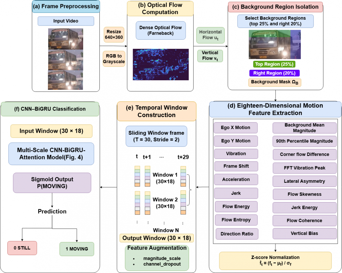
The proposed system operates on video data captured with CCTV cameras, which are mounted on the exterior side wall of the bus and mainly focus on the footboard and door region. This arrangement allows the camera to capture the bus structure as well as the surrounding environment, such as the road surface, platform area, and nearby background objects. This is unlike interior surveillance, where global motion of the scene is caused by the movement of the bus, and local passenger motion is located near the footboard, requiring separation of the two. The overall methodology pipeline consists of main stages as frame preprocessing, estimation of optical flow, background isolation, feature extraction and temporal window formation, and classification using a hybrid CNN–BiGRU network, as illustrated in Figure 3. Mathematically, the input and output videos can be mapped as follows.
Let It be the sequence of video frames captured by a CCTV camera placed outside the bus, focused on the bus footboard area. The aim of the framework is to learn a mapping function that will predict the label of the motion class from the image as in Eq. (1).
$y=f\left(I_t\right) ; y \in[0,1]$ (1)
where, $y=\left\{\begin{array}{lr}1, & \text { MOVING}, \\ 0, & \text { STILL. }\end{array}\right.$
3.1 Frame preprocessing
The input video frames are resized to a fixed resolution of 640 × 360 pixels to get a consistent video frame size from various video recordings and to minimize computation. The frames are then converted from RGB to grayscale representation prior to motion estimation. This makes the colour information less redundant and retains the structural and motion information needed for optical flow computation (Figure 3(a–f)). In the preprocessing stage, all of the inputs are processed in a standardized way as seen in Figure 3(a), in order to ensure that all further steps are carried out with an equally standardized input.
Figure 3. Overview of the proposed Bus Dynamic Stream pipeline showing (a) frame preprocessing, (b) dense optical flow computation, (c) background isolation, (d) feature extraction, (e) temporal window construction, and (f) classification
3.2 Optical flow computation
Dense optical flow is calculated between the frames at positions t and (t + 1) and feature extraction is limited to specific background areas like the upper portion of the frame and the extreme lateral areas. These regions are then used to generate an extended set of motion descriptors. Several complementary descriptors of motion are extracted, including directional flow ratio, motion coherence, lateral asymmetry, percentile-based flow statistics, vertical motion bias, corner-region flow differences, jerk energy, and flow skewness. These descriptors not only capture the overall motion of the vehicle but also exhibit fine-grained temporal changes that cannot be represented by simple optical-flow statistics. These features present a simple but effective visualisation of vehicle dynamics. In order to model the temporal dependency between the features, a hybrid deep learning architecture composed of a one-dimensional convolutional neural network (1D-CNN) and a bidirectional gated recurrent unit (BiGRU) has been employed. While the CNN captures short-term fluctuations and local motion patterns, the BiGRU learns long-range temporal consistency, enabling robust classification under noisy and dynamic conditions.
Mathematically, the dense optical flow field between these frames is represented as in Eq. (2).
$\mathrm{F}_t(x, y)=\left(u_t(x, y), v_t(x, y)\right)$ (2)
where, $F_t(x, y)$ denotes the dense optical-flow vector at pixel location $(x, y)$ between frames $t$ and $t+1$. $u_t(x, y)$ and $v_t(x, y)$ represent the horizontal and vertical displacement components measured in pixels/frame. The image dimensions are $H \times W$. Since the objective is to estimate the motion of the bus rather than passenger activity, feature extraction is restricted to a predefined background region $\Omega_B \subset R^2$, selected such that it contains minimal human motion. The corresponding background flow set is defined as in Eq. (3).
$F_t^B=\left\{F_t(x, y) \mid(x, y) \in \Omega_B\right\}$ (3)
where, $\Omega_B \subset \mathbb{R}^2$ denotes the selected background region containing minimal passenger motion. Only pixels satisfying $(x, y) \in \Omega_B$ are used for feature extraction. From this background flow, a normalized feature vector ft∈ R18 is computed at each time step, capturing multiple aspects of motion dynamics including ego-motion, vibration, and higher-order temporal variations. Over a temporal window of length T = 30, the feature sequence is represented as in Eq. (4).
$X_i=\left[f_t, f_{t+1}, \ldots, f_{t+T-1}\right] \in R^{T \times 18}$ (4)
where, $f_t \in \mathbb{R}^{18}$ is the proposed 18-dimensional feature vector extracted from frame $t$. $T=30$ denotes the temporal window length and $X_i$ represents the input sequence corresponding to the $i^{th}$ training sample. The task of bus motion-state classification is then formulated as a binary classification problem shown in Eq. (5), where a mapping function $\Phi(\cdot)$ learns to predict the probability of the bus being in motion:
$\hat{y}_i=\Phi\left(X_i\right), \hat{y}_i \in[0,1]$ (5)
where, Φ(⋅) represents the proposed Multi-Scale Residual CNN-BiGRU-Attention network, $\hat{y}_i$ denotes the predicted probability that the $i^{th}$ temporal window belongs to the MOVING class, and the final class label is obtained using a threshold of 0.5. A formulation allows combining temporal dynamics and spatial motion cues in a single learning process framework. The Farneback algorithm is used because it gives a good balance between computational cost and dense motion estimation. This flow field contains both global motion caused by bus movement and local motion due to passengers. Dense motion estimation using the Farneback algorithm is computed using the following parameters: pyr_scale = 0.5, levels = 3, winsize = 15, iterations = 3, poly_n = 5, poly_sigma = 1.2. The resulting flow field is represented by the following Eq. (6).
$F \in R^{H * W * 2}$ (6)
where, H and W denote the frame height and width, respectively. The last dimension stores the horizontal (fx) and vertical (fy) optical-flow components for every pixel. This provides per-pixel motion vectors, where each vector consists of horizontal and vertical displacements (fx) and (fy) respectively measured in pixels per frame. Since our aim is to estimate only vehicle motion, further processing is required to isolate relevant regions, as shown in Figure 3(b).
3.3 Background isolation
To ensure that the extracted motion features reflect only the movement of the bus and not passenger activity, feature extraction is restricted to selected background regions. Since the CCTV camera is mounted externally and rigidly fixed to the bus body, the selected regions typically include:
(1) The upper portion of the frame (sky or distant background), and
(2) The extreme right portion (roadside or static structures), which typically contain minimal passenger activity.
Let $\Omega_B \subset R^2$ denote the selected background region. The corresponding background optical flow is defined as in Eq. (7).
$F_B^t=\left\{F_t(x, y) \mid(x, y) \in \Omega_B\right\}$ (7)
where, $F_B^t$ represents the optical-flow vectors extracted only from the selected background region. This ensures that only motion vectors corresponding to global scene motion are considered. Since the camera is rigidly attached to the bus, consistent motion observed in these regions directly reflects the ego-motion of the vehicle. This spatial masking reduces the influence of passenger motion and improves robustness, as shown in Figure 3(c).
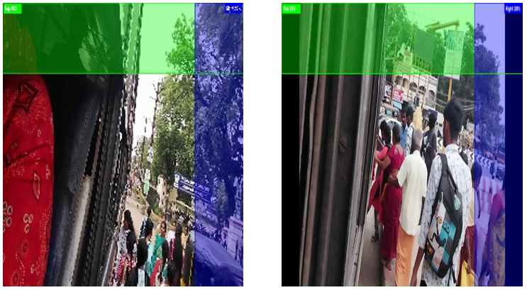
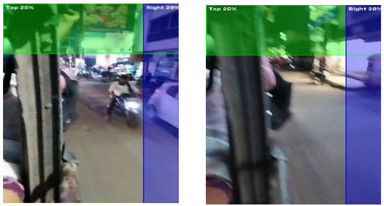
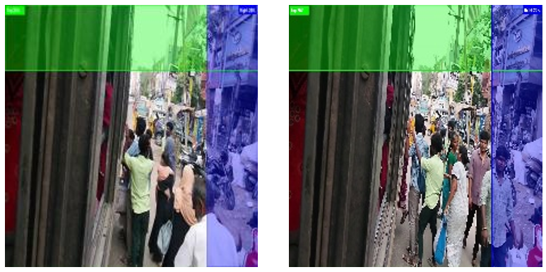
The background regions used in this work were selected based on repeated visual observation of the training videos. During preliminary analysis, passenger movement was consistently concentrated around the entrance and lower central portion of the frame, whereas the upper part and the extreme right side mainly contained distant background structures with very little passenger activity. Based on these observations, the upper 25% and the rightmost 20% of the frame were selected empirically and kept unchanged for all experiments, as shown in Figure 4. Occasionally, moving roadside vehicles, tree branches, or temporary occlusions may appear within these regions. However, such disturbances usually occupy only a small portion of the selected background area and therefore have limited influence on the aggregated motion descriptors computed over each temporal window.
From a mathematical point of view, the proposed background isolation can be interpreted as a spatial filtering operation applied over the optical flow field. Specifically, a binary mask corresponding to $\Omega_B$ suppresses foreground motion components caused by passengers, while preserving background motion vectors that are consistent with camera displacement. As the camera is rigidly attached to the bus body, this filtered flow field provides a direct approximation of vehicle ego-motion without requiring explicit geometric modelling or camera calibration.
3.4 Enhanced motion feature extraction
From the background optical flow $F_B^t$, a set of physics-based features is extracted for each frame to describe bus motion.
The magnitude of optical flow is computed as shown in Eq. (8).
$\begin{aligned} & M^t(x, y)=\sqrt{\left(f_x^t(x, y)\right)^2+\left(f_y^t(x, y)\right)^2} \text { for all }(x, y) \in \Omega_B \end{aligned}$ (8)
where, $M^t(x, y)$ denotes the optical-flow magnitude at pixel location $(x, y)$. The magnitude is computed only for pixels belonging to the background region $\Omega_B$. These features (Table 3) capture translation, vibration, and higher-order motion changes, helping to distinguish real bus motion from passenger disturbances. Note that the selected features are not arbitrary but are selected to represent different levels of dynamics of motion. The components of the ego-motion describe first-order translations; vibration captures stochastic variations of the flow magnitude, while higher-order temporal derivatives of the motion are described by acceleration and jerk. This hierarchical structure allows the system to differentiate between continuous vehicle motion and transient disturbances like passenger motion and short-term noises. The basic motion descriptors are further complemented using additional statistical and directional flow measurements. These include direction ratio, flow coherence, lateral asymmetry, 90th-percentile flow magnitude, vertical motion bias, corner-region flow difference, jerk energy, and flow skewness. While the original descriptors capture translation and temporal dynamics, the additional features characterize flow consistency, directional dominance, spatial imbalance, and higher-order motion distributions. Together, they provide a richer representation of bus dynamics under crowded and noisy operating conditions.
Table 3. Enhanced optical-flow descriptors extracted from the selected background region
|
S. No. |
Feature |
Equation |
Calculation Range |
Description |
|
1 |
Ego Motion X |
$median_{(x, y) \in \Omega_B} f_x^t(x, y)$ |
All $(x, y) \in \Omega_B$ |
Median horizontal optical flow in the background region |
|
2 |
Ego Motion Y |
$median_{(x, y) \in \Omega_B} f_y^t(x, y)$ |
All $(x, y) \in \Omega_B$ |
Median vertical optical flow in the background region |
|
3 |
Vibration |
$vibration^t=std_{(x, y) \in \Omega_B} M^t(x, y)$ |
All $(x, y) \in \Omega_B$ |
Standard deviation of optical-flow magnitude |
|
4 |
Frame Shift |
$\sqrt{\left(e g o_x^t-e g o_x^{t-1}\right)^2+\left(e g o_y^t-e g o_y^{t-1}\right)^2}$ |
Consecutive frames $(t-1, t)$ |
Ego-motion displacement between consecutive frames |
|
5 |
Acceleration |
$\begin{aligned} \mid{mean}_{(x, y) \in \Omega_B} M^t & (x, y)-{mean}_{(x, y) \in \Omega_B} M^{t-1}(x, y) \mid\end{aligned}$ |
Consecutive frames $(t-1, t)$ |
Temporal change in motion magnitude |
|
6 |
Jerk |
$\mid accel ^t- accel ^{t-1} \mid$ |
Three consecutive frames $(t-1, t)$ |
Change in acceleration |
|
7 |
Background Mean Magnitude |
$mean_{(x, y) \in \Omega_B} M^t(x, y)$ |
All $(x, y) \in \Omega_B$ |
Mean optical-flow magnitude in the background region |
|
8 |
Flow Energy |
$\sum_{i=1}^N M_i^2$ |
All $(x, y) \in \Omega_B$ |
Total optical-flow energy |
|
9 |
FFT Vibration Peak |
$\max \left(\left|F\left(M_i\right)\right|\right)$ |
Temporal window $(T=30)$ frames |
FFT(vibration) |
|
10 |
Flow Entropy |
$H=-\sum_{i=1}^N p_i \log \left(p_i\right)$ where $p_i=\frac{M_i}{\sum_{j=1}^N M_j}$ |
All $(x, y) \in \Omega_B$ |
Randomness of optical-flow magnitude distribution |
|
11 |
Direction Ratio |
$\frac{1}{N} \sum_{i=1}^N 1\left(v_i>0\right)$ |
All $(x, y) \in \Omega_B$ |
Fraction of pixels having positive vertical flow |
|
12 |
Flow Coherence |
$\frac{1}{N} \sum_{i=1}^N \frac{u_i \hat{d}_x+v_i \hat{d}_y}{M_i}$ where $\hat{d}=\frac{(\bar{u}, \bar{v})}{\sqrt{\bar{u}^2+\bar{v}^2}}$ |
All $(x, y) \in \Omega_B$ |
Directional consistency with dominant flow direction |
|
13 |
Lateral Asymmetry |
$\begin{gathered}\left|\mu_L-\mu_R\right| \text { where } \mu_L= mean\left(b_x^{left}\right) ; \\ \mu_R=mean\left(b_x^{\text {right }}\right)\end{gathered}$ |
Left and right background regions $\left(\Omega_B^L, \Omega_B^R\right)$ |
Left-right motion difference |
|
14 |
90th Percentile Magnitude |
$\operatorname{Percentile}_{90}\left(M_i\right)$ |
All $(x, y) \in \Omega_B$ |
Upper-tail motion magnitude |
|
15 |
Vertical Bias |
$\frac{\left|{mean}\left(b_y\right)\right|}{\left|mean\left(b_x\right)\right|+\epsilon}$ |
All $(x, y) \in \Omega_B$ |
Upper-tail optical-flow magnitude |
|
16 |
Corner Flow Difference |
$\begin{gathered}\left|\mu_{T L}-\mu_{T R}\right| \text { where } \mu_{T L}= { mean }\left(b_y^{T L}\right) ; \\ \mu_{T R}={mean}\left(b_y^{T R}\right)\end{gathered}$ |
Top-left and top-right regions $\left(\Omega_B^{T L}, \Omega_B^{T R}\right)$ |
Corner-region motion difference |
|
17 |
Jerk Energy |
$J_t^2$ |
Three consecutive frames $(t-2, t-1, t)$ |
Energy of jerk signal |
|
18 |
Flow Skewness |
$\frac{1}{N} \sum_{i=1}^N\left(\frac{M_i-\mu}{\sigma}\right)^3$ |
All $(x, y) \in \Omega_B$ |
Asymmetry of optical-flow magnitude distribution |
Normalization: Each feature is normalized using Z-score normalization Eq. (9):
$\hat{f}^t=\frac{f^t-\mu_f}{\sigma_f}$ (9)
where, $\mu_f$ and $\sigma_f$ denote the mean and standard deviation of the corresponding feature computed only from the training dataset. The normalized feature $\hat{f}^t$ has zero mean and unit variance. The feature extraction pipeline is shown in Figure 3(d). The complete mathematical definitions of the 18 motion descriptors extracted from the background optical-flow field are summarized in Table 3. These descriptors include statistical, directional, and temporal features that characterize bus motion under different operating conditions. Statistical descriptors are computed from the optical-flow vectors within the selected background region, whereas temporal descriptors are computed using consecutive frames or temporal windows.
In Table 3, $N$ denotes the total number of pixels in the selected background region $\Omega_B$, and $M_i$ represents the opticalflow magnitude of the $i^{\text {th }}$ background pixel. The symbols $\mu$ and $\sigma$ denote the mean and standard deviation of the opticalflow magnitude, respectively. The quantities $\mu_L$ and $\mu_R$ represent the mean horizontal optical flow in the left and right background regions, while $\mu_{T L}$ and $\mu_{T R}$ denote the mean vertical optical flow in the top-left and top-right background regions. The variables $b_x$ and $b_y$ denote the horizontal and vertical optical-flow components, respectively. The unit vector $\hat{d}$ represents the dominant flow direction estimated from the average background flow, and $\varepsilon$ is a small positive constant used to avoid division by zero.
Acceleration is computed as the absolute difference between the mean optical-flow magnitudes of two consecutive frames, while jerk is obtained as the absolute difference between two successive acceleration values. The FFT vibration peak is calculated by applying the Fast Fourier Transform (FFT) to the temporal vibration signal within each temporal window and selecting the maximum spectral magnitude. Flow entropy is computed from the normalized optical-flow magnitude distribution. Flow coherence measures the directional consistency between the optical-flow vectors and the dominant background motion direction. Corner-flow difference is calculated as the absolute difference between the average vertical optical flow in the top-left and top-right background regions. Flow skewness is computed as the third standardized moment of the optical-flow magnitude distribution.
3.5 Temporal window construction
Since bus motion is temporal, frame-wise features are grouped into overlapping windows. A stride of two frames is used to generate overlapping windows. The proposed feature vector contains 18 motion descriptors computed for every frame. Statistical descriptors are calculated over all pixels belonging to the selected background region, whereas temporal descriptors are computed using consecutive frames.
The smaller stride increases temporal overlap between adjacent windows and enables finer tracking of motion transitions, particularly during slow bus movement and intermittent stopping events. This allows the model to capture both short-term and long-term motion patterns, as shown in Figure 3(e). The use of overlapping temporal windows ensures that motion continuity is preserved across adjacent segments. This design avoids sudden transitions between windows and allows the model to capture gradual changes in motion patterns, which is particularly important in situations involving slow bus movement or intermittent stops.
3.6 CNN–BiGRU architecture
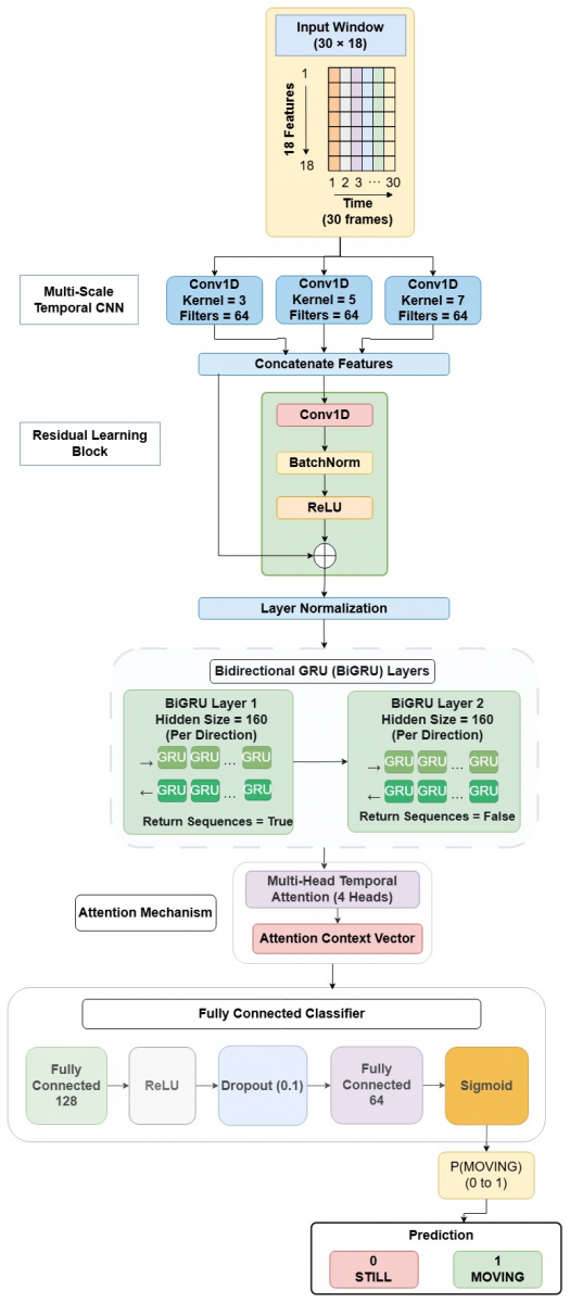
A hybrid CNN–BiGRU model (Figure 5) processes each temporal window. Each input window consists of 30 consecutive frames, where each frame is represented by an 18-dimensional feature vector. The CNN component employs a multi-scale temporal learning architecture comprising three parallel one-dimensional convolution (Conv1D) branches with kernel sizes of 3, 5, and 7, respectively. Each branch contains 64 filters to capture motion patterns at different temporal scales. Unless otherwise specified, all Conv1D layers employ a stride of 1 with same padding to preserve the temporal sequence length during feature extraction. Batch Normalization is applied after each convolution layer, followed by the ReLU activation function to improve training stability and nonlinear feature learning. The outputs of the three parallel convolution branches are concatenated and passed through a residual learning block consisting of a Conv1D layer, Batch Normalization, and ReLU activation with an identity skip connection to improve feature propagation and facilitate deeper temporal representation learning. Layer Normalization is subsequently applied to further improve training stability and reduce internal covariate shift. The extracted temporal features are then processed using two stacked BiGRU layers, each with 160 hidden units in each direction. The first BiGRU layer returns the complete sequence of hidden representations, whereas the second BiGRU layer outputs the final temporal representation for classification. A multi-head temporal attention module with four attention heads is then employed to emphasize the most informative temporal segments by generating an attention context vector.
Figure 5. Proposed multi-scale residual CNN-BiGRU-Attention architecture for bus motion-state classification
The attention context vector is passed to a fully connected classification module consisting of a 128-neuron fully connected layer, followed by ReLU activation, Dropout (0.1), and a second 64-neuron fully connected layer. Finally, a sigmoid activation function produces the probability of the two bus motion states, namely MOVING and STILL. This hybrid architecture effectively models both short-term local motion patterns and long-term temporal dependencies while highlighting the most informative temporal features before classification. The prediction is given by Eq. (10):
$\hat{y}=\sigma\left(W_0 h+b_0\right)$ (10)
where,
W0 denotes the weight matrix,
b0 denotes the bias term,
W0 and b0 are learnable parameters,
σ(・) represents the sigmoid activation function.
3.7 Training configuration
The model is trained using binary cross-entropy (BCE) loss:
$L=-\frac{1}{N} \sum_{i=1}^N\left[y_i \log \left(\hat{y}_i\right)+\left(1-y_i\right) \log \left(1-\hat{y}_i\right)\right]$ (11)
where, $y_i \in\{0,1\}$ is the ground truth label and $\hat{y}_i$ is the predicted probability.
Training uses the AdamW optimizer with a learning rate of $10^{-3}$, weight decay of $10^{-4}$, and a batch size of 64. A cosine annealing scheduler is used to improve convergence, and gradient clipping (maximum norm = 1.0) is applied to stabilize BiGRU training. AdamW with cosine annealing provides stable convergence and reduces overfitting, while gradient clipping improves numerical stability for long temporal sequences. Although the dataset is balanced at the video level, each video is divided into overlapping temporal windows (window length = 30 frames, stride = 2 frames). Since videos have different durations, the number of generated windows varies, causing moderate imbalance at the window level. Therefore, Weighted Random Sampler is used only for the training windows to create balanced mini-batches without changing the original video distribution. The proposed network has 1,465,409 trainable parameters. It is implemented in PyTorch and trained on Google Colab for a maximum of 120 epochs. Early stopping with a patience of 10 epochs is applied based on the validation loss, and the model with the lowest validation loss is selected for final testing. Training stability is verified using three random seeds (42, 7, and 123). Data augmentation, including magnitude scaling and channel dropout, is used to improve generalization. These augmentations simulate realistic optical-flow intensity variations and improve feature reliability under practical deployment conditions.
4.1 Classification performance
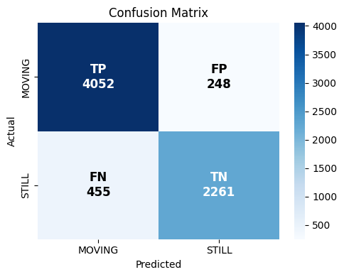
The proposed Bus Dynamic Stream model is evaluated on a separate test set of 60 videos with 0.500 as the threshold. The classification performance metrics reported in Table 4 are calculated at the temporal-window level. Since each test video generates multiple overlapping temporal windows, the total number of evaluation samples is greater than the number of original videos. The proposed framework achieves an overall accuracy of 89.98% with a macro F1-score of 0.893, indicating balanced classification performance for both classes. It can be observed that the MOVING class achieves a higher F1-score (0.920) than the STILL class (0.866). This is mainly due to false-positive predictions in stationary scenes, particularly during heavy passenger boarding. In such situations, collective passenger movement produces optical-flow patterns that are similar to vehicle motion. However, the proposed background-region isolation strategy reduces the influence of passenger movement and enables the extracted motion features to better represent the actual motion of the bus. Figure 6 shows the confusion matrix of the proposed model. The model correctly classifies most MOVING and STILL samples, with only a small number of misclassifications. The confusion statistics indicate that the model shows slightly higher sensitivity for the MOVING class than the STILL class. This behaviour is acceptable for safety-related applications, where misclassifying a moving bus as still is more critical than the reverse case.
Table 4. Classification metrics at threshold=0.500
|
Class |
Precision |
Recall |
F1-Score |
Accuracy |
Support |
|
STILL (0) |
0.833 |
0.901 |
0.866 |
– |
2509 |
|
MOVING (1) |
0.942 |
0.899 |
0.920 |
– |
4507 |
|
Macro Average |
0.888 |
0.900 |
0.893 |
– |
7016 |
|
Overall |
– |
– |
– |
0.8998 |
7016 |
Figure 6. Confusion matrix for bus motion-state classification showing true positives, true negatives, false positives, and false negatives
In addition to the window-level evaluation, video-level prediction was obtained using majority voting across all temporal windows belonging to each video. The video-level evaluation showed a performance trend similar to the window-level results, indicating that the proposed framework produces consistent predictions throughout the video sequence.
4.2 Video-level performance evaluation
To check the practical performance of the proposed method, video-level classification was also carried out. The final class for each test video was decided by majority voting of all temporal windows extracted from that video. The sliding-window method used a window length of 30 frames and a stride of 2 frames, so each test video produced multiple overlapping windows. Short videos were classified using all the available windows. No tie cases were observed during the evaluation.
Table 5 presents the video-level performance of the proposed framework. The video-level evaluation achieved comparable performance and slightly higher overall accuracy because majority voting reduces isolated window-level misclassifications. This shows that the proposed method gives stable and reliable results when the whole video is used.
Table 5. Video-level performance of the proposed framework
|
Metric |
Value |
|
Accuracy |
0.9160 |
|
Precision |
0.9100 |
|
Recall |
0.9085 |
|
F1-score |
0.9085 |
|
AUC-ROC |
0.9150 |
Note: AUC-ROC = Area Under the Curve–Receiver Operating Characteristic.
4.3 Area Under the Curve–Receiver Operating Characteristic analysis and threshold behavior
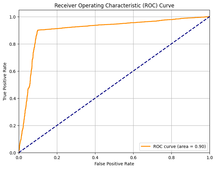
The proposed model was trained using three different random seeds to evaluate its training stability. Receiver Operating Characteristic (ROC) analysis was performed to assess the discrimination capability of the model without depending on a fixed classification threshold. A summary of the results is presented in Table 6. The proposed model achieved an AUC-ROC of 0.9001, indicating good discrimination between the MOVING and STILL classes. The optimal operating threshold obtained using the Youden J statistic is 0.8002, with a True Positive Rate (TPR) of 0.8989 and a False Positive Rate (FPR) of 0.0983. This threshold is close to the default threshold of 0.500, indicating that the model outputs are reasonably well calibrated. These results show that the learned temporal motion representation effectively separates the two motion classes without requiring complex threshold tuning.
Table 6. AUC-ROC analysis summary
|
Metric |
Value |
|
AUC-ROC |
0.9001 |
|
Optimal Threshold (Youden J) |
0.8002 |
|
TPR at Optimal |
0.8987 |
|
FPR at Optimal |
0.0983 |
|
Overall Accuracy (thr = 0.500) |
0.8989 |
|
Macro F1 (thr = 0.500) |
0.8933 |
Note: AUC-ROC = Area Under the Curve–Receiver Operating Characteristic; TPR = True Positive Rate; FPR = False Positive Rate; thr = Threshold.
Figure 7 shows the ROC curve of the proposed model. The curve demonstrates good classification performance over different threshold values. The higher-order motion descriptors, particularly acceleration and jerk, improve the discrimination capability of the proposed feature representation, resulting in better separation between the MOVING and STILL classes.
Figure 7. Receiver Operating Characteristic (ROC) curve for model performance evaluation
4.4 Hyperparameter sensitivity analysis
A one-at-a-time hyperparameter analysis was conducted to study the sensitivity of the proposed model to key design parameters. The results are presented in Table 7. Among the evaluated parameters, the temporal window size has the most significant impact on the classification performance.
Table 7. Parameter tuning results
|
Configuration |
Dropout |
Window Size |
Validation Accuracy |
Δ Accuracy |
|
Baseline |
0.10 |
30 |
0.8998 |
0.0000 |
|
Dropout = 0.25 |
0.25 |
30 |
0.8514 |
-0.0486 |
|
Window Size = 15 |
0.10 |
15 |
0.8500 |
-0.0500 |
|
Window Size = 25 |
0.10 |
25 |
0.8383 |
-0.0617 |
|
Learning Rate = 0.0005 |
0.10 |
30 |
0.8396 |
-0.0604 |
|
Learning Rate = 0.0010 |
0.10 |
30 |
0.8543 |
-0.0457 |
The sensitivity analysis shows that the proposed framework is moderately influenced by changes in temporal window size, dropout regularization, and learning rate. Among the evaluated parameters, the temporal window size produced the largest impact on performance, indicating the importance of temporal context for reliable bus motion-state classification. The baseline configuration achieved the highest validation accuracy of 90.0%.
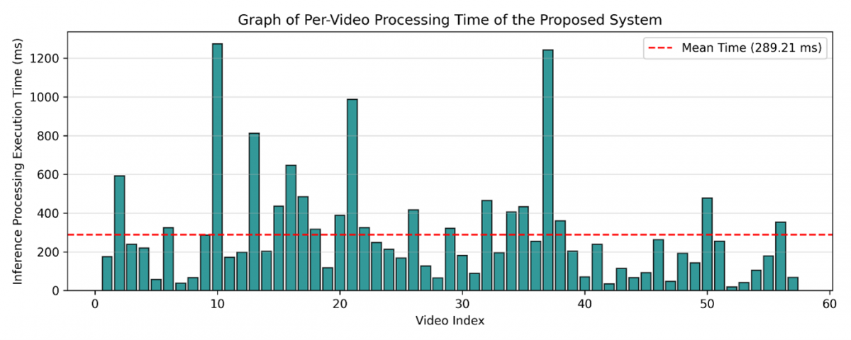
Figure 8 shows the graphical comparison of the processing time for the input videos. Deviations from the baseline configuration generally resulted in reduced performance, confirming that the selected hyperparameters provide a suitable balance between temporal representation learning and model generalization.
Figure 8. Graph of per-video processing time of the proposed system
4.5 Comparison with baseline methods
For a fair comparison, all learning-based baseline methods were trained using the same 18-dimensional motion feature vectors extracted from the optical-flow analysis. The same sliding-window settings (window length = 30 frames, stride = 2 frames) were used for all temporal models. Hyperparameters were selected using the validation set before testing. All methods were evaluated on the same training, validation, and test splits, ensuring that performance was measured on the same unseen videos. The Optical Flow Threshold method was applied directly to the optical-flow measurements without learning and was included as a conventional baseline for comparison.
The performance comparison presented in Table 8 shows that the proposed model achieved the highest overall performance with an accuracy of 89.98%, a macro F1-score of 0.893, and an AUC-ROC of 0.9001. Traditional machine learning methods, such as Logistic Regression, SVM, and Random Forest, produced lower performance, indicating the limitations of handcrafted motion features in capturing complex temporal dynamics. Similarly, the standalone LSTM and BiGRU models achieved lower accuracy than the proposed framework. The improved performance of the proposed model demonstrates the effectiveness of combining multi-scale CNN feature extraction with BiGRU-based temporal sequence learning for bus motion-state classification.
Table 8. Performance comparison of the proposed model with baseline methods
|
Method |
Accuracy |
F1 Score |
AUC-ROC |
|
Optical Flow Threshold |
0.500 |
0.3333 |
0.7089 |
|
Logistic Regression |
0.6667 |
0.6606 |
0.7611 |
|
Random Forest |
0.7167 |
0.7166 |
0.8022 |
|
SVM (18 features) |
0.6500 |
0.6476 |
0.7756 |
|
LSTM |
0.6833 |
0.6811 |
0.7833 |
|
BiGRU only |
0.6667 |
0.6652 |
0.7922 |
|
Proposed model |
0.8998 |
0.893 |
0.9001 |
Note: SVM = Support Vector Machine; LSTM = Long Short-Term Memory; BiGRU = Bidirectional Gated Recurrent Unit; AUC-ROC = Area Under the Curve–Receiver Operating Characteristic.
4.6 Runtime performance and practical feasibility
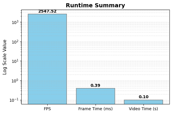
The runtime of the proposed system was evaluated on a CPU using Google Colab, and the results are shown in Table 9. The system processed 15,734 frames from 60 test videos in 6.18 seconds, with an average speed of 2547.52 FPS during the feature extraction and classification stages, excluding dense optical-flow computation. The reported runtime does not include frame resizing or dense Farneback optical-flow computation, as these stages were not separately profiled. The proposed framework reduces the downstream computational cost through compact feature aggregation and lightweight temporal modelling.
Table 9. Runtime performance of the proposed framework on a Central Processing Unit (CPU) using Google Colab
|
Performance Metric |
Value |
|
Test videos |
60 |
|
Processed frames |
15,734 |
|
Processing time (s) |
6.18 |
|
Processing speed (FPS) |
2547.52 |
|
Time per frame (ms) |
0.39 |
|
Time per video (s) |
0.10 |
The reported runtime shows that the proposed feature extraction and classification framework is computationally efficient after dense optical-flow computation. Since frame resizing and dense optical-flow estimation were not profiled separately, no claim is made about the end-to-end runtime or onboard deployment of the complete system. Figure 9 shows the runtime summary of the evaluated processing stages.
Figure 9. Runtime summary of the proposed system
4.7 Temporal smoothing analysis
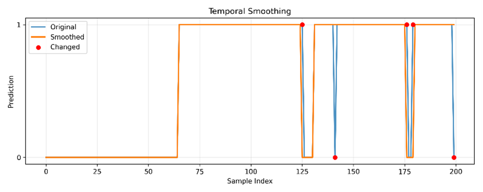
Temporal smoothing improves the classification performance by reducing false positives and increasing true negatives without affecting the true positive and false negative rates. This improves the stability of the predictions by suppressing transient fluctuations, particularly in shorter or noisier sequences. A comparison of the original and smoothed predictions is shown in Figure 10, where temporal smoothing reduces abrupt fluctuations in the prediction sequence.
Figure 10. Effect of temporal smoothing analysis
The smoothed output is more stable, with fewer isolated misclassifications, resulting in improved overall classification performance. To improve prediction stability, temporal smoothing is applied over a sliding window of size K. The smoothed prediction at time t is computed as the average of the previous K predictions. The final binary decision is then obtained by thresholding the averaged value. Alternatively, majority voting can be used to select the most frequent label within the sliding window. Temporal smoothing improves the stability of window-level predictions and reduces transient fluctuations. To incorporate temporal consistency, the smoothed prediction $\tilde{y}_t$ is computed over a sliding window of size K as shown in Eq. (12).
$\tilde{y}_t=\frac{1}{K} \sum_{k=0}^{K-1} \hat{y}_{t-k}$ (12)
The final class label $y_t$ is then obtained by thresholding the averaged value as in Eq. (13).
$y_t= \begin{cases}1, & \text { if }\ \tilde{y}_t>0.5, \\ 0, & \text { otherwise} .\end{cases}$ (13)
Alternatively, a majority voting scheme can be employed, where the final prediction is given by Eq. (14).
$y_t={mode}\left(\hat{y}_t, \hat{y}_{t-1}, \ldots, \hat{y}_{t-K+1}\right)$ (14)
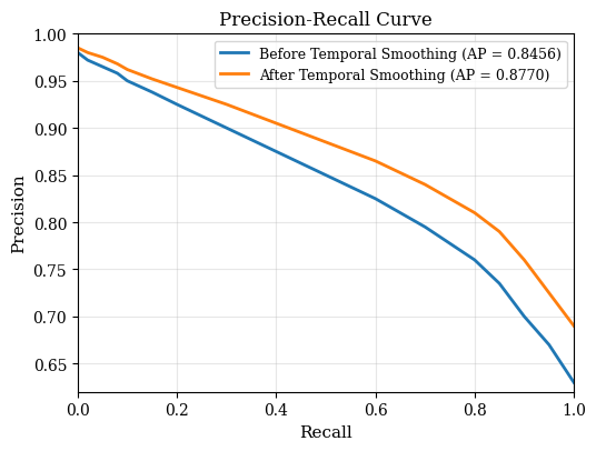
This temporal smoothing strategy reduces noisy fluctuations in the prediction sequence and improves consistency across consecutive temporal windows, as illustrated in Figure 11.
Figure 11. Precision–recall curve before and after temporal smoothing
4.8 Failure case analysis
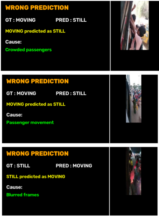
The misclassified samples were studied to understand where the proposed method makes mistakes. Figure 12 shows some failure cases from the unseen test dataset. Most false-positive errors happen when the bus is not moving and many passengers are getting in or out. The movement of several passengers creates strong optical flow. This looks similar to the motion of a moving bus. So, some stationary frames are wrongly classified as MOVING. Most false-negative errors happen when the bus moves very slowly. In this case, the bus motion is very small. The optical flow becomes weak and is difficult to separate from small background changes. Similar errors also happen when moving roadside objects appear near the selected background region and create extra motion. In a few cases, camera vibration, blurred frames, or temporary blockage of the selected background region affect the optical flow estimation. These cases are rare in our dataset, but they can reduce the classification accuracy. Overall, the proposed method works well in normal conditions. Most errors occur only in crowded boarding scenes or when the bus moves very slowly. In future work, adaptive background-region selection and additional scene information will be used to improve the robustness of the method.
Figure 12. Misclassified samples
4.9 Ablation study
To evaluate the contribution of each major component of the proposed framework, an ablation study was performed by removing one component at a time while keeping all other training and testing settings unchanged. The evaluated variants include the removal of background masking, jerk, acceleration, BiGRU, and temporal smoothing. All models were trained and evaluated using the same training, validation, and testing datasets to ensure a fair comparison. Table 10 presents the contribution of each major component of the proposed framework. The proposed model achieves the highest performance with an accuracy of 89.98%, a macro F1-score of 0.893, and an AUC-ROC of 0.9001. Removing background isolation significantly reduces the performance, indicating that background-region isolation is important for reducing the influence of passenger movement during motion estimation.
Table 10. Ablation study of bus dynamics features
|
S. No. |
Variant |
Accuracy |
F1-Score |
AUC-ROC |
|
1 |
Proposed Model |
0.8998 |
0.8930 |
0.9001 |
|
2 |
Without Background Masking |
0.7018 |
0.7018 |
0.7906 |
|
3 |
Without Jerk |
0.7544 |
0.7537 |
0.8042 |
|
4 |
Without Acceleration |
0.6842 |
0.6841 |
0.7833 |
|
5 |
CNN Only (without BiGRU) |
0.6842 |
0.6841 |
0.7882 |
|
6 |
Without Attention |
0.8500 |
0.8400 |
0.8600 |
|
7 |
Without Temporal Smoothing |
0.7368 |
0.7368 |
0.8042 |
Note: S. No. = Serial Number; CNN = Convolutional Neural Network; BiGRU = Bidirectional Gated Recurrent Unit; AUC-ROC = Area Under the Curve–Receiver Operating Characteristic.
The removal of jerk and acceleration features also decreases the performance, showing that higher-order motion descriptors provide useful information for distinguishing MOVING and STILL conditions. The CNN-only model without BiGRU shows a considerable performance reduction, demonstrating the importance of temporal sequence learning for capturing motion variations across consecutive windows. Similarly, removing the attention mechanism decreases the performance from 0.8998 to 0.8500 accuracy, indicating that the attention module helps in selecting more informative temporal features. The absence of temporal smoothing also reduces the performance due to increased prediction fluctuations. Overall, the ablation results confirm that background isolation, motion descriptors, temporal learning, attention, and smoothing collectively contribute to the improved performance of the proposed framework.
This paper presents Bus Dynamic Stream, a background-isolated temporal learning method to classify a bus as MOVING or STILL using videos from an exterior CCTV camera. Unlike conventional optical-flow methods that use the whole frame, the proposed method extracts motion only from selected background regions where passenger movement is minimal. This reduces the effect of passenger motion and gives motion information that better represents the actual bus movement. The extracted background optical flow is converted into an 18-dimensional temporal feature and analysed using a Multi-Scale Residual CNN-BiGRU-Attention network. The method was tested on 400 videos collected from 50 buses. It achieved an accuracy of 89.98%, a macro F1-score of 0.893, and an AUC-ROC of 0.9001. These results show that combining background isolation with temporal deep learning improves bus motion-state classification. The reported results are valid only for the dataset and camera setup used in this study. The method has not been tested on other bus models, different camera positions, viewing angles, weather conditions, night-time videos, or datasets from other cities. Future work will test the method on larger and more diverse datasets, develop adaptive background-region selection for different camera views, and extend the framework for more detailed vehicle motion and passenger behaviour analysis.
[1] Horn, B.K.P., Schunck, B.G. (1981). Determining optical flow. Artificial Intelligence, 17(1-3): 185-203. https://doi.org/10.1016/0004-3702(81)90024-2
[2] Zhang, C.X., Ge, L.Y., Chen, Z., Li, M., Liu, W., Chen, H. (2020). Refined TV-L1 optical flow estimation using joint filtering. IEEE Transactions on Multimedia, 22(2): 349-364. https://doi.org/10.1109/TMM.2019.2929934
[3] Scaramuzza, D., Fraundorfer, F. (2011). Visual odometry [tutorial]. IEEE Robotics & Automation Magazine, 18(4): 80-92. https://doi.org/10.1109/MRA.2011.943233
[4] Zhao, B.G., Huang, Y.P., Wei, H.J., Hu, X. (2021). Ego-motion estimation using recurrent convolutional neural networks through optical flow learning. Electronics, 10(3): 222. https://doi.org/10.3390/electronics10030222
[5] Mahdian, N., Jani, M., Enayati, A.M.S., Najjaran, H. (2024). Ego-motion aware target prediction module for robust multi-object tracking. arXiv preprint arXiv:2404.03110. https://doi.org/10.48550/arXiv.2404.03110
[6] Rajarathinam, G., Rajakannan, R., Chinnasamy, R., et al. (2026). A hybrid CNN-BiLSTM model for real-time activity classification in distributed acoustic sensing systems. Traitement du Signal, 43(2): 641-647. https://doi.org/10.18280/ts.430207
[7] Duja, K.U., Khan, I.A., Alsuhaibani, M. (2024). Video surveillance anomaly detection: A review on deep learning benchmarks. IEEE Access, 12: 164811-164842. https://doi.org/10.1109/ACCESS.2024.3491868
[8] Wang, H., Schmid, C. (2013). Action recognition with improved trajectories. In 2013 IEEE International Conference on Computer Vision, Sydney, NSW, Australia, pp. 3551-3558. https://doi.org/10.1109/ICCV.2013.441
[9] Donahue, J., Hendricks, L.A., Guadarrama, S., Rohrbach, M., Venugopalan, S., Darrell, T. (2015). Long-term recurrent convolutional networks for visual recognition and description. In 2015 IEEE Conference on Computer Vision and Pattern Recognition (CVPR), Boston, MA, USA, pp. 2625-2634. https://doi.org/10.1109/CVPR.2015.7298878
[10] Simonyan, K., Zisserman, A. (2014). Two-stream convolutional networks for action recognition in videos. In Proceedings of the 28th International Conference on Neural Information Processing Systems, Montreal, Canada, pp. 568-576. https://dl.acm.org/doi/10.5555/2968826.2968890.
[11] Liang, K. (2026). A video image processing approach for classroom interaction detection and dynamic teaching quality evaluation in english instruction. Traitement du Signal, 43(2): 615-628. https://doi.org/10.18280/ts.430205
[12] Chapel, M.N., Bouwmans, T. (2020). Moving objects detection with a moving camera: A comprehensive review. Computer Science Review, 38: 100310. https://doi.org/10.1016/j.cosrev.2020.100310
[13] Mur-Artal, R., Montiel, J.M.M., Tardós, J.D. (2015). ORB-SLAM: A versatile and accurate monocular SLAM system. IEEE Transactions on Robotics, 31(5): 1147-1163. https://doi.org/10.1109/TRO.2015.2463671
[14] Vijayanarasimhan, S., Ricco, S., Schmid, C., Sukthankar, R., Fragkiadaki, K. (2017). SfM-Net: Learning of structure and motion from video. arXiv preprint arXiv:1704.07804. https://doi.org/10.48550/arXiv.1704.07804
[15] Kirillov, A., He, K.M., Girshick, R., Rother, C., Dollár, P. (2019). Panoptic segmentation. In 2019 IEEE/CVF Conference on Computer Vision and Pattern Recognition (CVPR), Long Beach, CA, USA, pp. 9396-9405. https://doi.org/10.1109/CVPR.2019.00963
[16] Hong, S., Noh, H., Han, B. (2015). Decoupled deep neural network for semi-supervised semantic segmentation. In Proceedings of the 29th International Conference on Neural Information Processing Systems, Montreal, Canada, pp. 1495-1503. https://dl.acm.org/doi/10.5555/2969239.2969406.
[17] Hartley, R., Zisserman, A. (2004). Multiple View Geometry in Computer Vision. 2nd ed. Cambridge University Press. https://doi.org/10.1017/CBO9780511811685
[18] Vaswani, A., Shazeer, N., Parmar, N., et al. (2017). Attention is all you need. In Proceedings of the 31st International Conference on Neural Information Processing Systems, Long Beach, California, USA, pp. 6000-6010. https://dl.acm.org/doi/10.5555/3295222.3295349.
[19] Arnab, A., Dehghani, M., Heigold, G., Sun, C., Lučić, M., Schmid, C. (2021). ViViT: A video vision transformer. In: Proceedings of the IEEE/CVF International Conference on Computer Vision (ICCV), Montreal, Canada, pp. 6836-6846. https://doi.org/10.1109/ICCV48922.2021.00678
[20] Shi, X.J., Chen, Z.R., Wang, H., Yeung, D.Y., Wong, W.K., Woo, W.C. (2015). Convolutional LSTM network: A machine learning approach for precipitation nowcasting. In Proceedings of the 29th International Conference on Neural Information Processing Systems, Montreal, Canada, pp. 802-810. https://dl.acm.org/doi/10.5555/2969239.2969329.
[21] Feichtenhofer, C., Fan, H.Q., Li, Y.H., He, K.M. (2022). Masked autoencoders as spatiotemporal learners. In Proceedings of the 36th International Conference on Neural Information Processing Systems, New Orleans, LA, USA, pp. 35946-35958. https://dl.acm.org/doi/10.5555/3600270.3602875.
[22] Schuster, M., Paliwal, K.K. (1997). Bidirectional recurrent neural networks. IEEE transactions on Signal Processing, 45(11): 2673-2681. https://doi.org/10.1109/78.650093