Jing Li | Tingting Huang | Meng Wang | Ning Zhang* | Junjie Ma
© 2026 The authors. This article is published by IIETA and is licensed under the CC BY 4.0 license (http://creativecommons.org/licenses/by/4.0/).
OPEN ACCESS
High-accuracy remote sensing of water quality parameters, particularly chlorophyll-a (Chl-a) concentration and turbidity, is essential for monitoring inflowing river reaches of inland reservoirs. A water quality retrieval framework integrating multi-source hyperspectral imagery and deep learning was developed. A coordinated satellite–airborne–ground observation system was established by integrating unmanned aerial vehicle hyperspectral imagery (170 bands, 400–1000 nm) with GaoFen-5 (GF-5) satellite hyperspectral imagery (330 bands, 400–2500 nm) acquired over the upstream inflow reaches of the Yanghe Reservoir in Qinhuangdao, China. During image preprocessing, radiometric calibration, Fast Line-of-sight Atmospheric Analysis of Spectral Hypercubes (FLAASH) atmospheric correction, precise geometric registration, and resampling were sequentially performed to achieve spatial alignment and spectral band matching among the multi-source images. Subsequently, 11 key spectral reflectance features were extracted and concatenated at the pixel level to construct a 22-dimensional fused feature vector. To characterize both local dependencies and global patterns within the spectral feature sequence, a one-dimensional convolutional neural network was developed and benchmarked against a multilayer perceptron. Model training and optimization were performed using the Smooth L1 loss function, the AdamW optimizer, and Optuna-based automated hyperparameter optimization, while model performance was evaluated using stratified K-fold cross-validation. The results demonstrated that multi-source hyperspectral image fusion substantially improved turbidity retrieval accuracy. For turbidity retrieval, the one-dimensional convolutional neural network achieved a coefficient of determination (R²) of 0.896 and a root mean square error (RMSE) of 0.777 NTU, outperforming the multilayer perceptron and effectively mitigating the spectral saturation observed in high-concentration waters when single-source imagery was used. Notably, GF-5 imagery alone also exhibited excellent performance for Chl-a retrieval, with higher accuracy than the fused dataset, whereas the multilayer perceptron remained robust under small-sample conditions. These findings reveal parameter-specific differences in the suitability of different data sources: multi-source fusion is more suitable for turbidity retrieval, whereas GF-5 imagery alone provides superior performance for Chl-a retrieval. Overall, the results demonstrate the effectiveness of combining multi-source hyperspectral image fusion with deep-learning-based spectral sequence modeling for fine-scale water quality parameter retrieval and provide a transferable image-processing framework for remote sensing applications in aquatic environmental monitoring.
hyperspectral image fusion, multi-source remote sensing image registration, one-dimensional convolutional neural network, spectral feature extraction, chlorophyll-a concentration retrieval, turbidity retrieval
With the rapid advancement of global industrialization and urbanization, water pollution and ecological degradation have been recognized as global environmental challenges [1, 2]. As key optically active water quality parameters characterizing eutrophic status and suspended solids content in water bodies, chlorophyll-a (Chl-a) and turbidity require accurate and dynamic monitoring, which is of great significance for water quality assessment, algal bloom early warning, and aquatic ecological management [3-6]. Although high accuracy is provided by traditional point-based sampling and laboratory-based water quality monitoring methods, these methods are constrained by long monitoring durations, limited spatial coverage, and high costs, and the requirements for high-frequency, dynamic monitoring of large-scale water bodies cannot be met [7]. Although continuous observation capacity is provided by automated monitoring stations, their widespread deployment in small- and medium-sized watersheds has been restricted by high construction, operation, and maintenance costs [8]. Therefore, the development of an efficient, low-cost, and wide-coverage water quality monitoring technology system has become an urgent need for current water environment governance.
Remote sensing technology, by virtue of its advantages of noncontact, wide-area, and high-frequency observation, has been established as an important complement to traditional water quality monitoring methods [4, 9, 10]. Among these, detailed spectral information can be acquired by hyperspectral remote sensing, and spectral differences caused by concentration changes in Chl-a, suspended solids, and other components can be captured more sensitively, thereby facilitating the construction of more accurate water quality parameter retrieval models [11-14]. However, hyperspectral remote sensing is still constrained by limited spatial resolution, susceptibility to interference from the optical complexity of water bodies (e.g., water depth, substrate reflectance, and water surface fluctuation), and complex data preprocessing workflows, by which the robustness and applicability of retrieval models are restricted [15, 16].
In recent years, great potential has been demonstrated by unmanned aerial vehicle hyperspectral technology for accurate monitoring of small- and medium-scale water bodies, owing to its high spatial resolution and flexible maneuverability [17, 18]. However, spatiotemporal coverage is limited by the endurance and field of view of a single platform. Multi-source remote sensing data fusion is considered an effective approach for improving retrieval accuracy and robustness, and preliminary progress has been made in the synergistic use of hyperspectral and multispectral data, optical and synthetic aperture radar data, and other data combinations [8, 19].
In terms of retrieval models, traditional empirical models have been gradually replaced by machine learning and deep learning methods, and nonlinear relationships between remote sensing reflectance spectra and water quality parameters can be effectively characterized [20-22]. Significantly superior accuracy has been demonstrated by deep-learning-based Chl-a retrieval models compared with traditional methods, and stronger generalization ability has been observed in complex water environments [23-26]. However, systematic research on collaborative modeling of multi-source data, coupling mechanisms among parameters, and model interpretability remains relatively lacking, as most existing studies have been concentrated on single-source data or single-parameter retrieval.
On the basis of the above research status and limitations, the upstream inflow river reach of the Yanghe Reservoir was selected as a typical study area. Unmanned aerial vehicle hyperspectral data and satellite hyperspectral data were fused, and deep learning algorithms were incorporated to systematically compare the performance differences of different data sources in Chl-a and turbidity retrieval. An efficient water quality monitoring system suitable for small- and medium-scale water bodies was constructed, by which high-frequency dynamic monitoring of Chl-a and turbidity was achieved; the deficiencies of traditional methods in spatiotemporal resolution and monitoring frequency were compensated for; and a low-cost, intelligent, and generalizable technical pathway was provided for regional water environment and ecological protection. The main contributions of this study are as follows: (i) By constructing a coordinated satellite–unmanned aerial vehicle–ground observation scheme over the upstream inflow reach of the Yanghe Reservoir and systematically comparing single-source and fused retrieval under identical conditions, we reveal a parameter-specific data-source matching pattern: multi-source fusion is preferable for turbidity retrieval, whereas GaoFen-5 (GF-5) imagery alone outperforms the fused dataset for Chl-a retrieval; (ii) this finding provides a directly transferable, cost-saving data-selection strategy for high-frequency monitoring of small- and medium-scale inflow reaches; and (iii) the reproducible pixel-level band-alignment workflow between 5-cm unmanned aerial vehicle hyperspectral imagery and 30-m GF-5 AHSI imagery is documented to support similar applications.
2.1 Study area overview
The Yanghe Reservoir is located in the northwestern part of Qinhuangdao City, Hebei Province (119°15′–119°30′E, 40°00′–40°15′N). A watershed area of approximately 755 km² is controlled by the reservoir, which is recognized as an important drinking water source for the region. Water from multiple inflow river channels is received by the reservoir, and pronounced spatiotemporal variations in water quality are observed, which are jointly affected by agricultural nonpoint source pollution, shoreline human activities, and seasonal hydrological conditions.
Three major inflow river channels of the Yanghe Reservoir were selected as key monitoring areas. A total of 80 sampling sites were established at typical inflow inlets and shoreline zones so that external pollution input pathways, water exchange and diffusion processes, and water quality differences under different shoreline environments could be represented. The specific location of the study area and the sampling site layout are shown in Figures 1 and 2.

Figure 1. Overview of the study area

Figure 2. Spatial distribution of sampling sites (red dots)
2.2 Data acquisition
For the construction of a high-accuracy water quality retrieval model, multi-source data were collected in April 2025 at the Yanghe Reservoir in Qinhuangdao. These data comprised unmanned aerial vehicle hyperspectral imagery, synchronous in situ water sampling, and GaoFen-5 (GF-5) satellite hyperspectral imagery so that temporal and spatial consistency of the model training samples was ensured.
2.2.1 Unmanned aerial vehicle hyperspectral imagery acquisition
Hyperspectral data were acquired using a DJI unmanned aerial vehicle platform equipped with an independently developed visible–near-infrared imaging spectrometer. A spectral range of 400–1000 nm and 170 contiguous narrowband spectral channels were provided by the instrument. A spatial resolution of approximately 5 cm was achieved at a flight altitude of 300 m. The flight mission was completed in April 2025 over the three major upstream inflow river channels of the Yanghe Reservoir during a single acquisition. The main inflow estuaries and typical shoreline areas were covered by the imagery, and differential Global Positioning System (GPS) was used for flight-line control, by which spatial matching and positioning accuracy between the imagery and in situ samples were ensured.
2.2.2 GaoFen-5 satellite hyperspectral data acquisition
To further enhance the regional scalability and temporal gap-filling capability of the retrieval model, GF-5 satellite hyperspectral imagery was acquired in parallel. The Advanced Hyperspectral Imager (AHSI) onboard the satellite covers 400–2500 nm, with 330 contiguous spectral channels, a spectral resolution better than 5 nm, and a spatial resolution of 30 m.
A GF-5 image covering the Yanghe Reservoir area on April 10, 2025, was selected. This date was close to the unmanned aerial vehicle flight and in situ sampling dates, and cloud cover was less than 10%, so consistency between the water quality conditions reflected by the imagery and actual field conditions was ensured.
2.2.3 Synchronous in situ water quality sampling
To support model development and validation for the retrieval model, 80 in situ sampling sites were established within the remote sensing coverage area. The spatial distribution of these sites was designed to account for hydrodynamic gradients, water quality transition zones, and human activity-affected areas. All sites were positioned using high-precision GPS, and positioning errors were controlled within ±1 m.

Figure 3. Histograms of chlorophyll-a (Chl-a) concentration and turbidity at the sampling sites in the Yanghe Reservoir
Sampling was performed at a uniform depth of 0.4–0.8 m below the water surface. Samples were collected in brown glass bottles and rinsed five times with ambient water prior to collection to prevent cross-contamination. Following collection, samples were immediately sealed, shielded from light, stored at 0–4 ℃, and transported to the laboratory within 24 h under cold-chain conditions. Parallel determinations were performed for all water quality indicators, and measurement errors were controlled within 5%.
To characterize the distribution of water quality parameters at the sampling sites, histograms of Chl-a and turbidity were generated (Figure 3). A unimodal distribution was exhibited by Chl-a, with concentrations mainly concentrated between 0.9 and 1.6 μg/L and few extreme values, indicating that the trophic status of the reservoir was relatively stable during the sampling period. A pronounced right-skewed distribution was exhibited by turbidity, with most samples distributed between 0.9 and 2.0 NTU and some elevated values observed, indicating that the water body was generally clean but that locally elevated suspended solids concentrations were present. The overall sample distribution was balanced, and a reliable data foundation for water quality retrieval modeling was thereby provided.
2.3 Data preprocessing
To ensure the consistency and usability of data from different sources, standardized preprocessing was separately performed on satellite and unmanned aerial vehicle imagery data.
2.3.1 Radiometric calibration and atmospheric correction
Radiometric calibration is the process by which raw digital number values recorded in imagery are converted into absolute radiance, and sensor-related errors can thereby be mitigated. Radiometric calibration was implemented by determining the gain and offset, as expressed in Eqs. (1) and (2):
$L e^{\prime}=K \times D N+T$ (1)
$L e=\frac{L e^{\prime}}{\sin \left(\theta_{S E}\right)}$ (2)
where, Le is the apparent radiance (W·m⁻²·μm⁻¹·sr⁻¹); K is the absolute radiometric calibration gain coefficient (W·m⁻²·μm⁻¹·sr⁻¹); T is the absolute radiometric calibration offset coefficient (W·m⁻²·μm⁻¹·sr⁻¹); and θSE is the solar elevation angle.
Solar radiation is transmitted through the atmosphere, incident on the surface of ground objects, and then reflected back to the sensor. The received signal is disturbed by water vapor, aerosols, and adjacent ground objects, such that various interfering contributions other than the surface information of ground objects are introduced into the imagery. For the spectral properties of ground objects to be accurately extracted, these interference contributions must be separated; this process is referred to as atmospheric correction. Atmospheric correction methods are commonly classified into four categories: image feature-based models, band characteristic-based models, empirical models, and atmospheric radiative transfer models, as expressed in Eq. (3):
$C=\left(\frac{A \beta}{1-\beta_e \alpha}\right)+\left(\frac{B \beta_e}{1-\beta_e \alpha}\right)+C \alpha$ (3)
where, β is the surface reflectance of the pixel; α is the spherical albedo of the atmosphere; βe is the mean surface reflectance of the surrounding area; Ca is radiance; and A and B are coefficients independent of the surface that vary with atmospheric and geometric conditions.
Radiometric calibration was performed on the data using ENVI software, and atmospheric correction was carried out using the Fast Line-of-sight Atmospheric Analysis of Spectral Hypercubes (FLAASH) module. Radiance values were thereby converted into surface reflectance, and the effects of atmospheric aerosols, water vapor, and other atmospheric constituents were removed. Throughout the subsequent analysis, surface reflectance was expressed as dimensionless values in the range [0, 1], and radiance was expressed in units of W·m⁻²·μm⁻¹·sr⁻¹, in accordance with common remote sensing conventions.
2.3.2 Geometric correction and image registration
To achieve spatial consistency among multi-source data and between remote sensing imagery and ground sampling sites, geometric correction and registration were performed separately for the GF-5 and unmanned aerial vehicle imagery. For the GF-5 data, systematic geometric correction was first conducted using satellite orbital parameters, after which fine registration was performed using regional ground control points. The projection was uniformly transformed to the WGS 84 / UTM Zone 50N coordinate system.
For the unmanned aerial vehicle data, georectification was completed based on flight trajectory information and control points with the support of position and orientation system/inertial measurement unit (POS/IMU) data. A spatial accuracy better than 1 m was achieved, by which precise matching with the sampling sites was ensured. All ground sampling site coordinates were transformed into the same unified UTM coordinate system, and spatial resampling was applied to ensure one-to-one correspondence between remote sensing pixels and sampling sites.
3.1 Feature band extraction
Although continuous and fine spectral resolution is provided by hyperspectral imagery, redundant and noisy bands are often contained in raw spectra. In particular, strong water vapor absorption bands in the near-infrared regions (e.g., near 940, 1130, and 1400 nm) are affected by atmospheric and sensor interference, and low and unstable signal-to-noise ratios are exhibited; therefore, systematic errors are readily introduced when direct modeling is performed. Accordingly, band screening was first performed on the unmanned aerial vehicle hyperspectral and GF-5 data to remove severely contaminated spectral intervals. Smoothing treatments, such as moving average or Savitzky–Golay filtering, were then applied, by which high-frequency noise was reduced and the continuity and stability of spectral curves were improved [27, 28].
To balance modeling accuracy and computational efficiency and to ensure comparability among different sensor data, 11 key bands (545, 554, 572, 600, 619, 671, 705, 724, 739, 761, and 829 nm) from the unmanned aerial vehicle hyperspectral imagery were selected as reference feature bands. The main water vapor absorption regions and high-noise regions are avoided by this combination, and a high signal-to-noise ratio and spectral stability are exhibited. Since the spectral resolution of the GF-5 AHSI is approximately 5 nm, the central channels closest to the aforementioned bands were selected from the GF-5 data, by which band correspondence and feature alignment among multi-source data were achieved, and providing a basis for collaborative modeling was provided.
Based on the above band selection strategy, the 11 spectral reflectance values from both unmanned aerial vehicle and GF-5 data were extracted at the locations of the in situ sampling sites, and these values were concatenated along the band dimension to form a 22-dimensional fused feature vector. A comparative experimental framework for multi-source fusion and single-source data was constructed, by which the sensitivity of unmanned aerial vehicle data to spectral details was preserved and the advantages of GF-5 data in regional coverage were incorporated, enabling systematic evaluation of the retrieval capabilities of different data sources for Chl-a and turbidity.
3.2 Development of deep learning models
To achieve high-accuracy remote sensing retrieval of water quality parameters (e.g., Chl-a concentration and turbidity) in the Yanghe Reservoir, one-dimensional convolutional neural network and multilayer perceptron models were constructed based on the previously acquired and preprocessed multi-source hyperspectral imagery and in situ measurements. The applicability and performance differences of different neural network architectures in hyperspectral water quality retrieval were thereby investigated [29, 30].
3.2.1 Construction of the one-dimensional convolutional neural network model
For each water sample, the hyperspectral reflectance was treated as a one-dimensional input sequence, and a one-dimensional convolutional neural network was constructed to automatically extract spectral features. Spectral information is compressed through convolution and pooling operations, spectral patterns associated with water quality indicators (e.g., absorption features and spectral shape) are learned, and predicted water quality parameters are output by a dense layer. Excellent performance has been demonstrated in capturing local spectral dependencies and in modeling with limited samples.
Three convolutional layers were included in the one-dimensional convolutional neural network model to extract local and long-range spectral features, and rectified linear unit activation functions and dropout layers were employed to prevent overfitting. Feature tensors output by the convolutional layers were flattened and fed into a fully connected module, which was composed of two linear layers, batch normalization, and activation functions so that nonlinear combinations of high-dimensional features could be achieved. Finally, the output layer, combined with global average pooling, produced the prediction of each water quality parameter; because Chl-a concentration and turbidity were modeled in two separate single-task networks, each network contained its own output layer that predicted a single scalar for the corresponding parameter (Figure 4).

Figure 4. Schematic diagram of the one-dimensional convolutional neural network architecture
3.2.2 Construction of the multilayer perceptron model
A feedforward architecture was primarily adopted for the multilayer perceptron. The input layer was initialized according to the concatenated feature dimension, and several hidden layers with decreasing dimensions were connected thereafter to achieve feature compression and nonlinear mapping. Each hidden layer was composed, in sequence, of a linear transformation, batch normalization, a leaky rectified linear unit with a negative slope of 0.2, and a dropout layer with a rate of 0.3 (Figure 5), so that robustness was enhanced and the risk of overfitting was reduced.
The output layer was composed of a linear mapping layer, by which raw regression values were directly output without any activation function. Since Chl-a and turbidity are continuous variables and were modeled separately, scalar predictions were directly provided by the output layer. An L1 regularization term with a strength coefficient of λ = 0.01 was introduced into the loss function to encourage parameter sparsity and to enhance model interpretability and generalization capability under multi-source high-dimensional features, and this term was incorporated into the optimization procedure through a weight-decay mechanism implemented in the optimizer.

Figure 5. Schematic diagram of the multilayer perceptron architecture
3.2.3 Model training and evaluation strategy
To enhance model generalization capability and to enable scientific performance evaluation, the following training strategy was adopted. In terms of data partitioning, all samples were divided into training and test sets at a ratio of 8:2. The 20% test set was held out before any modeling and was used only for the final performance evaluation; it was never involved in model training, hyperparameter tuning, or early stopping. The AdamW optimizer was employed for training, in combination with an adaptive learning rate and weight decay so that gradient explosion and overfitting were intended to be prevented. Smooth L1 loss was selected as the loss function, by which smoothness in the small-error regime and robustness in the large-error regime were both provided, and tolerance to outliers was improved.
The Optuna automatic hyperparameter tuning framework was integrated into model training. The search space included the number of hidden layers, the number of neurons, the dropout rate, the initial learning rate, and the L1 regularization strength. The optimal combination was automatically searched by the Tree-structured Parzen Estimator (TPE) Bayesian optimization, and training processes without improvement were terminated by an early stopping mechanism. To avoid optimistic bias, hyperparameter optimization and early stopping were performed exclusively on the training portion (80% of all samples) using the validation folds generated by the stratified cross-validation; the independent test set was excluded from all tuning and model-selection decisions.
Stratified K-fold cross-validation (K = 5) was adopted for training. To address the continuity of regression labels, log transformation and Z-score standardization were first applied to the target variables (Chl-a or turbidity), after which balanced stratified labels were generated by quantile discretization-based binning so that imbalanced effects of extreme sample values on training and validation partitioning were avoided. For the input features, Z-score standardization was applied to the 11 reflectance features of each data source (and, accordingly, to the 22-dimensional fused vector). To prevent information leakage, the mean and standard deviation of each feature were computed exclusively from the training fold within each cross-validation iteration and then applied to both the training and validation folds; the held-out test set was standardized using statistics derived only from the full training portion. Because the unmanned aerial vehicle and GF-5 sensors have different radiometric response ranges, standardization was performed independently for the features of each data source, thereby removing cross-sensor scale differences while preserving per-source statistical properties.
The above training procedure was consistently applied to both a multilayer perceptron and a one-dimensional convolutional neural network, by which performance comparability among different networks under identical conditions was ensured. For each target variable (Chl-a or turbidity), a dedicated single-task model was trained independently, and no multi-task joint training, loss weighting, or shared feature-extraction scheme was involved. In the evaluation stage, the regression performance of the two model types on Chl-a and turbidity was summarized separately, reflecting their applicability and differences in multi-source remote sensing water quality retrieval.
The final performance of the models was evaluated using the following three metrics:
Root mean square error (RMSE): The square root of the mean of the squared differences between the predicted and observed values. The overall deviation of predictions is reflected, with smaller values indicating higher accuracy, and relatively high sensitivity to outliers is exhibited.
$R M S E=\sqrt{\frac{1}{n} \sum_{i=1}^n\left(\hat{y}_i-y_i\right)^2}$
Mean absolute error (MAE): The mean of the absolute differences between predicted and observed values. The overall average error magnitude is directly reflected, and lower sensitivity to extreme values is exhibited.
$M A E=\frac{1}{n} \sum_{i=1}^n\left|\widehat{y}_i-y_i\right|$
Coefficient of determination (R²): The proportion of variance in the observed values explained by the model is measured. Values closer to 1 indicate a better fit.
$R^2=1-\frac{\sum_{i=1}^n\left(\hat{y}_i-y_i\right)^2}{\sum_{i=1}^n\left(\bar{y}_i-y_i\right)^2}$
3.3 Comparison of results from different data sources
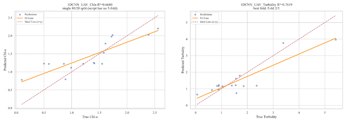
When only unmanned aerial vehicle hyperspectral single-source data were employed, certain predictive capability was exhibited by the model in the low-to-medium concentration range; however, pronounced saturation effects generally occurred in the medium-to-high concentration range, i.e., the ability of the model to resolve high-concentration water quality parameters was reduced because the spectral response flattened, often resulting in underestimation.
Table 1. Evaluation results of chlorophyll-a (Chl-a) prediction performance for both models under three input conditions (unit: μg/L)
|
Input Data |
Model |
Chl-a |
||
|
R² |
Root Mean Square Error (RMSE) |
Mean Absolute Error (MAE) |
||
|
Unmanned aerial vehicle (hyperspectral) |
One-dimensional convolutional neural network |
0.668 |
0.366 |
0.298 |
|
Multilayer perceptron |
0.540 |
0.446 |
0.346 |
|
|
GaoFen-5 (GF-5) (satellite) |
One-dimensional convolutional neural network |
0.983 |
0.081 |
0.063 |
|
Multilayer perceptron |
0.543 |
0.390 |
0.302 |
|
|
Unmanned aerial vehicle + GF-5 (fusion) |
One-dimensional convolutional neural network |
0.757 |
0.306 |
0.201 |
|
Multilayer perceptron |
0.641 |
0.372 |
0.260 |
|
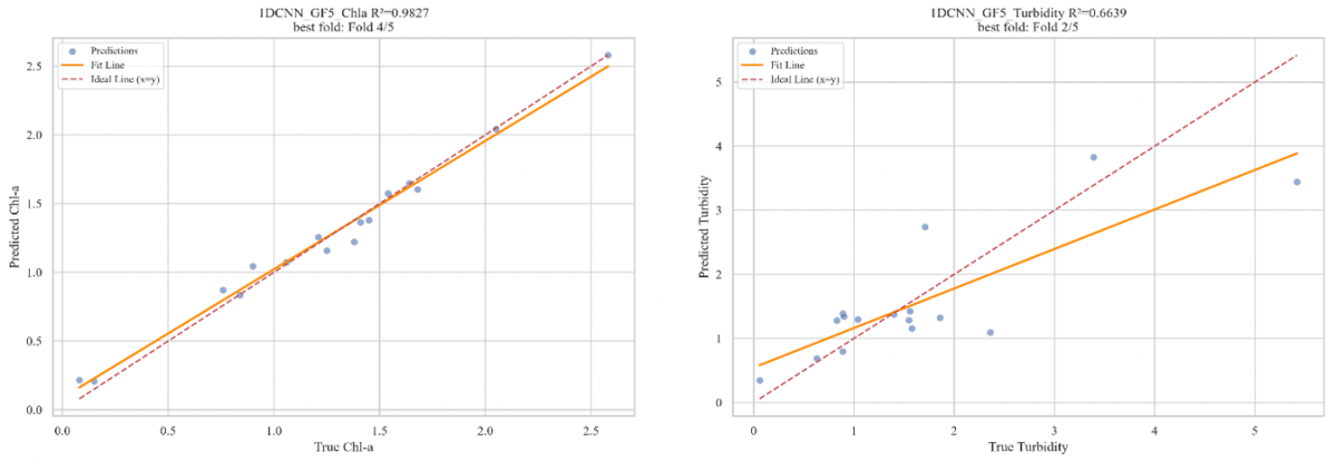
As shown in Tables 1 and 2, model performance in turbidity retrieval was significantly improved by the fused data, and generalization capability was stronger, particularly in the medium-to-high concentration interval. In contrast, for Chl-a retrieval, strong predictive capability was also demonstrated by GF-5 single-source data, and its accuracy was superior to that of the fusion results.
In comparison, the explained variance in turbidity retrieval was substantially improved by multi-source data fusion, although the accompanying RMSE and MAE were not reduced: the R² of the fused one-dimensional convolutional neural network for turbidity was increased to 0.896, and strong fitting capability was maintained across the entire concentration range, with the saturation effect of single-source data in the high-concentration interval being effectively alleviated. It should be noted that this improvement in R² was not accompanied by a reduction in RMSE (0.777 NTU vs. 0.600 NTU for the UAV single-source model) or MAE. This combination is not contradictory, because R² and RMSE emphasize different aspects of the error distribution: RMSE is dominated by the largest individual errors, and while fusion improved the overall fit and reduced high-concentration underestimation, it did not proportionally reduce the magnitude of the largest residuals. This improvement is attributed to the complementarity between unmanned aerial vehicle hyperspectral data and GF-5 data—subtle spectral absorption features are captured by the former with high spectral resolution, while overall background information is provided by the latter with broader spatial coverage. The problem of high local accuracy but weak overall generalization associated with single-source data was effectively alleviated by the combination of the two, enabling the model to achieve both local and overall prediction accuracy. In Chl-a retrieval, however, superior performance was exhibited by GF-5 single-source data, with prediction accuracy better than that of the fusion results, which may be related to the ability of the broader spectral coverage of the GF-5 AHSI to capture Chl-a-sensitive bands.
Table 2. Evaluation results of turbidity prediction performance for both models under three input conditions (unit: NTU)
|
Input Data |
Model |
Turbidity |
||
|
R² |
Root Mean Square Error (RMSE) |
Mean Absolute Error (MAE) |
||
|
Unmanned aerial vehicle (hyperspectral) |
One-dimensional convolutional neural network |
0.762 |
0.600 |
0.453 |
|
Multilayer perceptron |
0.779 |
0.456 |
0.362 |
|
|
GaoFen-5 (GF-5) (satellite) |
One-dimensional convolutional neural network |
0.664 |
0.713 |
0.512 |
|
Multilayer perceptron |
0.607 |
0.603 |
0.420 |
|
|
Unmanned aerial vehicle + GF-5 (fusion) |
One-dimensional convolutional neural network |
0.896 |
0.777 |
0.466 |
|
Multilayer perceptron |
0.709 |
1.301 |
0.636 |
|
Note: Results are the mean values across cross-validation folds; all values are reported to three decimal places.
Figure 6. Comparison of the predictive performance of both models for chlorophyll-a (Chl-a) concentration and turbidity using unmanned aerial vehicle hyperspectral data and GaoFen-5 (GF-5) satellite data
Overall, the high resolution of unmanned aerial vehicle hyperspectral data and the wide coverage of GF-5 satellite data were effectively combined by multi-source remote sensing data fusion, and the explained variance (R²) in turbidity retrieval was significantly improved across the entire concentration range and in high-disturbance areas, effectively mitigating the saturation effect of single-source data, while the error metrics (RMSE and MAE) were not reduced. Notably, excellent performance in Chl-a retrieval was also demonstrated by GF-5 single-source data, with accuracy even exceeding that of the fusion results. The significant improvement in retrieval accuracy in high-concentration areas by fusion techniques was also confirmed by Hong et al. [11], further demonstrating their advantages for parameter retrieval in complex dynamic water bodies. Figure 6 shows the comparison of the predictive performance of both models for Chl-a concentration and turbidity using unmanned aerial vehicle hyperspectral data and GF-5 satellite data.
3.4 Comparative analysis of model architectures
From the perspective of model architecture, pronounced advantages are exhibited by the one-dimensional convolutional neural network in processing high-dimensional continuous band data, owing to its local receptive field and hierarchical feature extraction mechanisms. Local dependencies among adjacent bands are automatically captured by its convolutional kernels, and higher-level features are abstracted through multiple convolutional layers, by which fitting accuracy and generalization capability are improved. On the fused data (Table 3), superior predictions of both Chl-a and turbidity were produced by the one-dimensional convolutional neural network compared with the multilayer perceptron, with test-set R² values of 0.757 and 0.896, respectively, which were significantly higher than those of the multilayer perceptron (0.641 and 0.709); lower RMSE and MAE values were also obtained. When the differences between training-set and test-set R² were examined, smaller training–test discrepancies were observed for the one-dimensional convolutional neural network than for the multilayer perceptron for both parameters (Chl-a: 0.971 vs. 0.757; turbidity: 0.958 vs. 0.896), indicating stronger generalization capability and a lower degree of overfitting for the one-dimensional convolutional neural network and demonstrating its greater advantage in learning complex hyperspectral features. This finding is consistent with the conclusion of Na et al. [31] that convolutional architectures are particularly suitable for sequence-based modeling of continuous spectral data.
Table 3. Performance metrics of both models for chlorophyll-a (Chl-a) and turbidity prediction based on fused unmanned aerial vehicle and GaoFen-5 (GF-5) data
|
Model |
Water Quality Parameter |
Training R² |
Test R² |
Root Mean Square Error (RMSE) |
Mean Absolute Error (MAE) |
|
One-dimensional convolutional neural network |
Chl-a |
0.971 |
0.757 |
0.306 |
0.201 |
|
Turbidity |
0.958 |
0.896 |
0.777 |
0.466 |
|
|
Multilayer perceptron |
Chl-a |
0.983 |
0.641 |
0.372 |
0.260 |
|
Turbidity |
0.934 |
0.709 |
1.301 |
0.636 |
Although inferior overall performance compared with the one-dimensional convolutional neural network was exhibited by the multilayer perceptron, more rapid convergence and greater noise robustness were provided by its fully connected architecture under conditions of limited sample size or strong noise. In the unmanned aerial vehicle single-source turbidity prediction experiment, the RMSE of the multilayer perceptron (0.456) was slightly lower than that of the one-dimensional convolutional neural network (0.600), which may be attributed to overfitting of the convolutional model under small-scale data, whereas global fitting relationships were learned more rapidly by the multilayer perceptron. This indicates that an efficient and stable baseline model is still provided by the multilayer perceptron when data are insufficient or resources are limited.
With respect to the large training–test discrepancy of the multilayer perceptron on Chl-a (training-set R² = 0.983 vs. test-set R² = 0.641 in Table 3), this gap indicates that the multilayer perceptron tended to overfit the small training sample under the high-dimensional fused input. Residual analysis and repeated-seed stability checks were therefore performed to assess this risk: the residuals were found to be concentrated in high-concentration samples without systematic bias, and the qualitative ranking of the two models was stable across repeated training runs. These diagnostics support the conclusion that the superior generalization of the one-dimensional convolutional neural network on fused data is reliable rather than an artifact of a single favorable data split.
From the perspectives of computational cost and application scenarios, greater practicality is offered by the multilayer perceptron because of its simple architecture, small number of parameters, and fast training speed when computing power is limited and rapid iteration or engineering deployment is required. Although higher complexity and longer training time are required by the one-dimensional convolutional neural network, pronounced advantages are exhibited in large-scale, high-accuracy water quality retrieval applications. Particularly when multi-source data are fused, data redundancy and noise interference are effectively alleviated by its multilayer convolutional feature extraction, and model stability and generalization capability are improved.
From the perspective of error distribution, superior fitting performance in high-concentration Chl-a and high-turbidity intervals was exhibited by the one-dimensional convolutional neural network, and the problems of traditional models in high-value intervals were effectively alleviated, whereas more pronounced deviations in these intervals were observed for the multilayer perceptron. This indicates that greater application value is provided by the one-dimensional convolutional neural network for monitoring highly polluted or highly eutrophic water bodies.
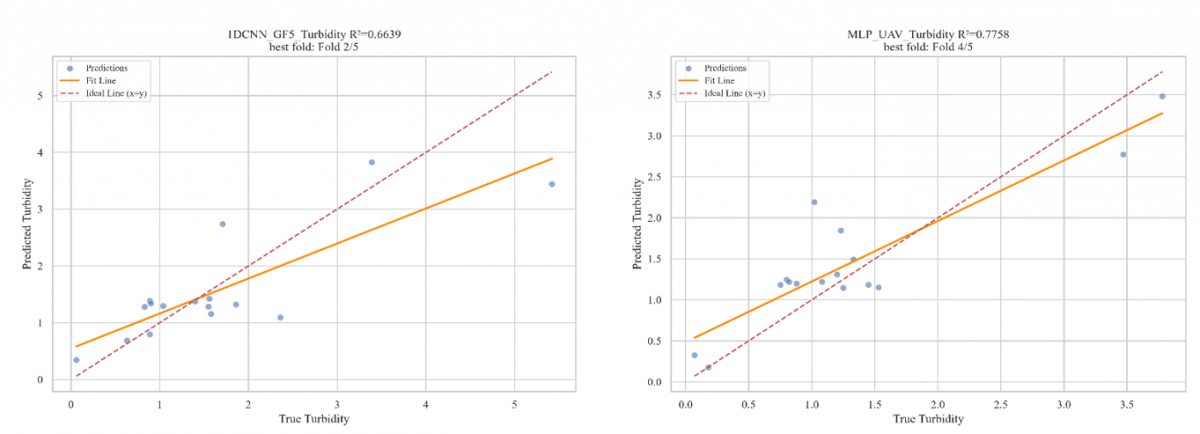
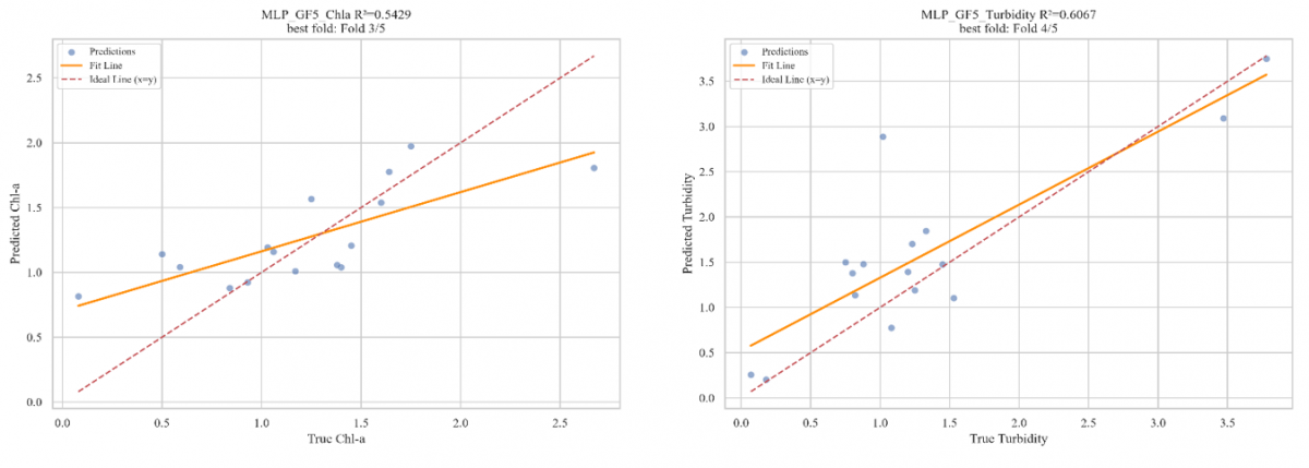
In summary, greater suitability for large-scale, high-accuracy remote sensing water quality retrieval tasks, particularly multi-source data modeling, is exhibited by the one-dimensional convolutional neural network, whereas the multilayer perceptron is more appropriate for rapid experimentation, resource-limited settings, or scenarios with relatively limited data volumes. The two model types are complementary and can be flexibly selected according to task objectives; integrated modeling of the two could be explored in future work so that the high accuracy of the convolutional neural network and the rapid convergence of the multilayer perceptron are both incorporated. Figure 7 shows the comparative performance of both models for Chl-a and turbidity prediction using fused unmanned aerial vehicle and GF-5 data.

Figure 7. Comparative performance of both models for chlorophyll-a (Chl-a) and turbidity prediction using fused unmanned aerial vehicle and GaoFen-5 (GF-5) data
A deep learning-based water quality parameter retrieval framework integrating unmanned aerial vehicle hyperspectral imagery and GF-5 satellite data was proposed for the Yanghe Reservoir in Qinhuangdao City. Modeling and accuracy assessment were conducted for two key indicators, Chl-a concentration and turbidity. The research findings and implications were discussed from three dimensions: the effectiveness of data fusion, the performance of model architectures, and the potential for practical application. In addition, the suitability patterns between different water quality parameters and data sources were revealed, thereby providing a scientific basis for data source selection in practical monitoring.
4.1 Superior Performance in turbidity retrieval achieved by multi-source data fusion
The high spatial resolution of unmanned aerial vehicle hyperspectral data and the wide coverage capability of GF-5 satellite data were effectively synergized by the fusion of these two data sources. It was shown that the explained variance in turbidity retrieval was significantly improved by the fused dataset (R² = 0.896 for the one-dimensional convolutional neural network), whereas the RMSE and MAE remained comparable and were not reduced, because RMSE is dominated by the largest individual errors and fusion mainly improved the overall fit and mitigated high-concentration saturation; superior response to water quality parameters in the medium-to-high concentration range was nevertheless achieved. In Chl-a retrieval, however, superior predictive performance was exhibited by GF-5 single-source data, with accuracy exceeding that of the fusion results. This apparent reduction of fusion performance for Chl-a is attributable to the limited sample size: the 22-dimensional fused feature vector superimposes largely redundant unmanned-aerial-vehicle bands on the already strong GF-5 signal, thereby increasing the input dimensionality and promoting overfitting under the small training sample; in contrast, for turbidity the high-spatial-resolution details provided by the unmanned-aerial-vehicle imagery contain genuinely complementary information that outweighs the dimensionality increase. The above results therefore suggest that the optimal data source should be selected for different water quality parameters. A flexible data selection strategy for water quality parameter retrieval is provided by the complementarity of multi-source data, by which single-source or fusion schemes can be selected according to target parameter characteristics. The limitations of a single platform in spatiotemporal resolution and spectral dimension were effectively overcome by the complementarity of multi-source data, and a reliable data foundation for robust water quality retrieval was thereby provided.
4.2 Outstanding performance achieved by the one-dimensional convolutional neural network model architecture
Among the compared deep learning architectures, outstanding performance was exhibited by the one-dimensional convolutional neural network. Local correlations between contiguous hyperspectral bands and global spectral patterns were efficiently captured, and locally sensitive features and global trends were collaboratively extracted through multi-scale convolutional kernels, by which more accurate and better-generalized retrieval of Chl-a and turbidity was achieved. Although simple in structure and computationally efficient, the multilayer perceptron was limited in retrieval accuracy because deep features of sequential spectral signals could not be effectively learned by its fully connected architecture, thereby confirming the inherent advantage of the one-dimensional convolutional neural network in processing hyperspectral data.
4.3 Practical applicability and deployment potential
Great potential for application in small- and medium-scale water body monitoring is exhibited by the flexible water quality monitoring strategy based on parameter–data source matching proposed herein. The optimal data source can be selected according to the characteristics of the target water quality parameter: for turbidity monitoring, fused unmanned aerial vehicle and GF-5 data are preferable for improving accuracy and generalization capability, whereas for Chl-a monitoring, GF-5 single-source data can be directly used to reduce cost and data processing complexity. This strategy is particularly suitable for fine-grained management of water bodies such as reservoirs, lakes, estuaries, and intensive aquaculture areas, with monitoring timeliness, spatial detail, and controllable cost being balanced. An efficient and generalizable technical pathway is thereby provided for high-frequency dynamic monitoring, algal bloom early warning, and pollution source tracing, and continuous data support can be provided for intelligent management decisions regarding regional water resources.
In this study, the upstream inflow river reach of the Yanghe Reservoir was selected as the study area, and a deep learning-based water quality retrieval framework integrating unmanned aerial vehicle hyperspectral imagery and GF-5 satellite data was constructed. The performance differences among different data sources in Chl-a and turbidity retrieval were systematically compared. The main conclusions are summarized as follows: (i) Significant advantages in turbidity retrieval were exhibited by multi-source data fusion. The test-set R² of the one-dimensional convolutional neural network model on the fused data reached 0.896, and the saturation effect of single-source data in the high-concentration range was effectively mitigated. (ii) In Chl-a retrieval, the prediction accuracy of GF-5 single-source data was superior to that of the fused data, suggesting that differences exist in the spectral responses of different water quality parameters to data sources, and the optimal data source should be selected according to the characteristics of the target parameter. (iii) The overall performance of the one-dimensional convolutional neural network model on the fused data was superior to that of multilayer perceptron, with a smaller training–test gap and stronger generalization capability, making it more suitable for modeling tasks involving continuous hyperspectral sequences. A reference basis for data source selection and model construction in remote sensing monitoring of water quality in small- and medium-scale water bodies is provided by these findings.
This paper was supported by Science Research Project of Hebei Education Department (Grant No.: CXZX2025060) and Project of Hebei University of Environmental Engineering (Grant No.: XJXM-QN-2024002).
[1] Ali, H., Khan, E., Ilahi, I. (2019). Environmental chemistry and ecotoxicology of hazardous heavy metals: Environmental persistence, toxicity, and bioaccumulation. Journal of Chemistry, 2019(1): 6730305. https://doi.org/10.1155/2019/6730305
[2] Huang, C.W., Chai, Z.Y., Yen, P.L., et al. (2020). The bioavailability and potential ecological risk of copper and zinc in river sediment are affected by seasonal variation and spatial distribution. Aquatic Toxicology, 227: 105604. https://doi.org/10.1016/j.aquatox.2020.105604
[3] Le, C., Li, Y., Zha, Y., Sun, D., Huang, C., Lu, H. (2009). A four-band semi-analytical model for estimating chlorophyll a in highly turbid lakes: The case of Taihu Lake, China. Remote Sensing of Environment, 113(6): 1175-1182. https://doi.org/10.1016/j.rse.2009.02.005
[4] Li, L., Li, L., Song, K., et al. (2013). An inversion model for deriving inherent optical properties of inland waters: Establishment, validation and application. Remote Sensing of Environment, 135: 150-166. https://doi.org/10.1016/j.rse.2013.03.031
[5] Park, Y., Cho, K.H., Park, J., Cha, S.M., Kim, J.H. (2015). Development of early-warning protocol for predicting chlorophyll-a concentration using machine learning models in freshwater and estuarine reservoirs, Korea. Science of the Total Environment, 502: 31-41. https://doi.org/10.1016/j.scitotenv.2014.09.005
[6] Yang, H., Kong, J., Hu, H., Du, Y., Gao, M., Chen, F. (2022). A review of remote sensing for water quality retrieval: Progress and challenges. Remote Sensing, 14(8): 1770. https://doi.org/10.3390/rs14081770
[7] Dörnhöfer, K., Oppelt, N. (2016). Remote sensing for lake research and monitoring–Recent advances. Ecological Indicators, 64: 105-122. https://doi.org/10.1016/j.ecolind.2015.12.009
[8] Kwon, D.H., Hong, S.M., Abbas, A., et al. (2023). Deep learning-based super-resolution for harmful algal bloom monitoring of inland water. GIScience & Remote Sensing, 60(1): 2249753. https://doi.org/10.1080/15481603.2023.2249753
[9] Cao, Q., Yu, G., Sun, S., Dou, Y., Li, H., Qiao, Z. (2021). Monitoring water quality of the Haihe River based on ground-based hyperspectral remote sensing. Water, 14(1): 22. https://doi.org/10.3390/w14010022
[10] Lim, J., Choi, M. (2015). Assessment of water quality based on Landsat 8 operational land imager associated with human activities in Korea. Environmental Monitoring and Assessment, 187(6): 384. https://doi.org/10.1007/s10661-015-4616-1
[11] Hong, S.M., Cho, K.H., Park, S., et al. (2022). Estimation of cyanobacteria pigments in the main rivers of South Korea using spatial attention convolutional neural network with hyperspectral imagery. GIScience & Remote Sensing, 59(1): 547-567. https://doi.org/10.1080/15481603.2022.2037887
[12] Cui, M., Sun, Y., Huang, C., Li, M. (2022). Water turbidity retrieval based on UAV hyperspectral remote sensing. Water, 14(1): 128. https://doi.org/10.3390/w14010128
[13] Judice, T.J., Widder, E.A., Falls, W.H., Avouris, D.M., Cristiano, D.J., Ortiz, J.D. (2020). Field-validated detection of aureoumbra lagunensis brown tide blooms in the Indian River Lagoon, Florida, using Sentinel-3A OLCI and ground-based hyperspectral spectroradiometers. GeoHealth, 4(6): e2019GH000238. https://doi.org/10.1029/2019GH000238
[14] Wu, J.L., Ho, C.R., Huang, C.C., Srivastav, A.L., Tzeng, J.H., Lin, Y.T. (2014). Hyperspectral sensing for turbid water quality monitoring in freshwater rivers: Empirical relationship between reflectance and turbidity and total solids. Sensors, 14(12): 22670-22688. https://doi.org/10.3390/s141222670
[15] Abdelmajeed, A.Y.A., Juszczak, R. (2024). Challenges and limitations of remote sensing applications in northern peatlands: Present and future prospects. Remote Sensing, 16(3): 591. https://doi.org/10.3390/rs16030591
[16] Chander, S., Gujrati, A., Krishna, A.V., Sahay, A., Singh, R.P. (2020). Remote sensing of inland water quality: A hyperspectral perspective. In Hyperspectral Remote Sensing, Elsevier, pp. 197-219. https://doi.org/10.1016/B978-0-08-102894-0.00017-6
[17] Xiao, Y., Guo, Y., Yin, G., et al. (2022). UAV multispectral image-based urban river water quality monitoring using stacked ensemble machine learning algorithms—A case study of the Zhanghe River, China. Remote Sensing, 14(14): 3272. https://doi.org/10.3390/rs14143272
[18] McEliece, R., Hinz, S., Guarini, J.M., Coston-Guarini, J. (2020). Evaluation of nearshore and offshore water quality assessment using UAV multispectral imagery. Remote Sensing, 12(14): 2258. https://doi.org/10.3390/rs12142258
[19] Zhang, Y., Pulliainen, J., Koponen, S., Hallikainen, M. (2002). Application of an empirical neural network to surface water quality estimation in the Gulf of Finland using combined optical data and microwave data. Remote Sensing of Environment, 81(2-3): 327-336. https://doi.org/10.1016/S0034-4257(02)00009-3
[20] Li, S., Song, K., Wang, S., et al. (2021). Quantification of chlorophyll-a in typical lakes across China using Sentinel-2 MSI imagery with machine learning algorithm. Science of the Total Environment, 778: 146271. https://doi.org/10.1016/j.scitotenv.2021.146271
[21] Hinton, G.E., Salakhutdinov, R.R. (2006). Reducing the dimensionality of data with neural networks. Science, 313(5786): 504-507. https://doi.org/10.1126/science.1127647
[22] Hu, X., Belle, J.H., Meng, X., et al. (2017). Estimating PM2.5 concentrations in the conterminous United States using the random forest approach. Environmental Science & Technology, 51(12): 6936-6944. https://doi.org/10.1021/acs.est.7b01210
[23] Gao, L., Shangguan, Y., Sun, Z., Shen, Q., Shi, Z. (2024). Estimation of non-optically active water quality parameters in Zhejiang province based on machine learning. Remote Sensing, 16(3): 514. https://doi.org/10.3390/rs16030514
[24] Hong, S.M., Morgan, B.J., Stocker, M.D., et al. (2024). Using machine learning models to estimate Escherichia coli concentration in an irrigation pond from water quality and drone-based RGB imagery data. Water Research, 260: 121861. https://doi.org/10.1016/j.watres.2024.121861
[25] Li, W., Fang, H., Qin, G., et al. (2020). Concentration estimation of dissolved oxygen in Pearl River Basin using input variable selection and machine learning techniques. Science of the Total Environment, 731: 139099. https://doi.org/10.1016/j.scitotenv.2020.139099
[26] Niu, C., Tan, K., Jia, X., Wang, X. (2021). Deep learning based regression for optically inactive inland water quality parameter estimation using airborne hyperspectral imagery. Environmental Pollution, 286: 117534. https://doi.org/10.1016/j.envpol.2021.117534
[27] Pafumi, E., Petruzzellis, F., Castello, M., et al. (2023). Using spectral diversity and heterogeneity measures to map habitat mosaics: An example from the Classical Karst. Applied Vegetation Science, 26(4): e12762. https://doi.org/10.1111/avsc.12762
[28] Zeng, K., Xu, Z., Yang, Y., et al. (2022). In situ hyperspectral characteristics and the discriminative ability of remote sensing to coral species in the South China Sea. GIScience & Remote Sensing, 59(1): 272-294. https://doi.org/10.1080/15481603.2022.2026641
[29] Alevizos, E. (2020). A combined machine learning and residual analysis approach for improved retrieval of shallow bathymetry from hyperspectral imagery and sparse ground truth data. Remote Sensing, 12(21): 3489. https://doi.org/10.3390/rs12213489
[30] Peterson, K.T., Sagan, V., Sloan, J.J. (2020). Deep learning-based water quality estimation and anomaly detection using Landsat-8/Sentinel-2 virtual constellation and cloud computing. GIScience & Remote Sensing, 57(4): 510-525. https://doi.org/10.1080/15481603.2020.1738061
[31] Na, X., Li, X., Li, W., Wu, C. (2021). Wetland mapping using HJ-1A/B hyperspectral images and an adaptive sparse constrained least squares linear spectral mixture model. Remote Sensing, 13(4): 751. https://doi.org/10.3390/rs13040751