Yi Wang
© 2026 The author. This article is published by IIETA and is licensed under the CC BY 4.0 license (http://creativecommons.org/licenses/by/4.0/).
OPEN ACCESS
The authentication of digital image evidence in judicial practice is increasingly challenged by sophisticated deep forgery techniques. Existing tampering localization methods often fail to reconcile pixel-level fine-grained perception with semantic-level evidentiary reasoning. Their limitations primarily stem from the shallow coupling of multi-scale frequency–spatial features, the semantic gap between localization outputs and factual case descriptions, and the lack of uncertainty quantification in reasoning processes. To address these challenges, this study proposes a unified framework for structure–semantic collaborative evidence reasoning. Specifically, a dynamic frequency–spatial multi-scale collaborative perception mechanism is designed, employing dynamically scaled perception units and a cross-scale non-rigid alignment module to achieve deep entanglement of frequency- and spatial-domain features. This enables the detection of tampering traces across scales—from large-scale semantic inconsistencies to subtle textural anomalies. Furthermore, a joint declarative–evidence attention mechanism and hierarchical contrastive learning strategy are introduced. By incorporating a Gradient Reversal Layer (GRL), visual features are enforced to conform to textual logical constraints, thereby enabling closed-loop optimization of tampering localization and cross-modal verification. To enhance interpretability, a variational Bayesian approximation combined with dynamic annular boundary constraints is adopted to generate a triple evidentiary report, comprising a tampering mask, a confidence heatmap, and a consistency score. Extensive experiments on public benchmarks and a self-constructed judicial evidence dataset demonstrate that the proposed method achieves state-of-the-art performance in localization accuracy, cross-domain generalization, and robustness against adversarial attacks. Notably, the evidence trustworthiness score significantly outperforms those of comparative methods, offering a reliable technical pathway for intelligent image authentication in forensic judicial contexts.
image tampering localization, cross-modal evidence verification, frequency–spatial feature fusion, uncertainty quantification, judicial digital evidence
Digital images occupy an increasingly critical position in the judicial proof system, where their authenticity and integrity directly determine the reliability of fact-finding in court cases [1, 2]. Meanwhile, deep learning-driven image editing and generation technologies are evolving at an unprecedented pace [3, 4]. Traditional tampering methods such as splicing, copy-move, and object removal have become highly sophisticated. Furthermore, semantic-level image forgeries enabled by Generative Adversarial Network (GAN) and diffusion models can generate visually flawless fake content, posing a fundamental challenge to traditional identification paradigms relying on human visual inspection [5, 6]. A series of judicial interpretations issued by the Supreme People’s Court explicitly list the verification of electronic data authenticity as a core step in judicial adjudication. However, current judicial practice still relies heavily on the subjective experience of forensic experts and limited automated auxiliary tools. Confronted with the increasing concealment and diversity of tampering techniques and the exponential growth in the volume of electronic evidence, the gap between existing forensic capabilities and judicial demands continues to widen. Consequently, developing intelligent image tampering detection and trustworthiness assessment methods tailored for judicial scenarios has become an urgent practical imperative [7, 8].
Recent years have witnessed significant progress in deep learning-based image tampering localization [9, 10]. However, existing methods still face three key bottlenecks when applied to the task of assessing the trustworthiness of judicial electronic evidence. First, the fusion depth of multi-scale frequency and spatial features remains insufficient [11, 12]. Most methods rely on single-scale spatial cues; even when frequency domain decomposition is introduced, frequency features are often treated merely as shallow supplements to spatial branches. Dynamic Frequency Former (DFFormer) integrates high- and low-frequency components via an adaptive frequency Transformer, yet the interaction between frequency and spatial features is limited to unidirectional transmission at specific network layers [13, 14]. Uncertainty and Frequency Guided Network (UFG-Net) utilizes uncertainty information to guide frequency domain feature extraction, but its dual-branch structure still lacks a deep bidirectional collaboration mechanism [15, 16]. How to achieve deep entanglement and dynamic collaboration between frequency and spatial domain features across multiple scales remains an unsolved problem [17, 18]. Second, a significant semantic gap exists between the tampering localization task and the requirements of judicial evidence examination. Existing methods output binary tampering masks, which can only indicate where an image has been manipulated. Judicial forensics, however, requires not only spatial localization but also answers to deeper questions, such as whether the tampered content is consistent with the factual description of the case and to what extent the tampering affects the probative value of the evidence [19, 20]. Although preliminary explorations in cross-modal fact verification have utilized the Contrastive Language–Image Pre-training (CLIP) model to achieve semantic alignment between text and multimodal evidence [21, 22], these applications are concentrated in news fact-checking and have not yet been organically integrated with pixel-level image tampering localization [23, 24]. Third, prediction results lack uncertainty quantification and interpretability support [25, 26]. Judicial evidence examination imposes stringent requirements on the reliability of conclusions, necessitating clear knowledge of the model’s confidence regarding its judgment on a specific region. Nevertheless, most existing tampering localization methods output deterministic binary predictions and lack quantitative assessment of predictive uncertainty [25, 26]. While UFG-Net utilizes uncertainty information during the training phase to guide feature extraction, it fails to output interpretable uncertainty metrics to users during inference. This deficiency severely restricts the credible application of deep learning models in judicial forensic practice [15, 25].
To address these shortcomings, this paper proposes a unified framework for structure-semantic collaborative evidence reasoning. The core contributions of this framework are threefold: (1) A dynamic frequency-spatial multi-scale collaborative perception mechanism is proposed. By employing dynamic scaling perception unit (DSPU) and a Cross-Scale Feature Alignment (CSFA) module, it achieves hierarchical deep entanglement of frequency and spatial domain features, effectively capturing cross-scale tampering traces ranging from large-scale semantic inconsistencies to small-scale textural anomalies. (2) A cross-modal evidence consistency verification module is constructed. Using visual anchors from tampering localization as indices, this module performs fine-grained semantic consistency checks between tampered regions and case text descriptions via declarative-evidence joint attention and hierarchical tampering contrastive learning. A Gradient Reversal Layer (GRL) is introduced to achieve closed-loop optimization where localization serves verification and verification, in turn, feeds back to localization. (3) A boundary-aware uncertainty learning and interpretable output layer is designed. Based on variational Bayesian approximation and Monte Carlo dropout inference, it outputs pixel-wise tampering probabilities, predictive entropy, and confidence intervals. Combined with a dynamic annular residual module to enhance the geometric precision of tampering boundaries, the framework ultimately generates a triple interpretable output comprising a tampering mask, a confidence heatmap, and a cross-modal consistency score.
The remainder of this paper is organized as follows: Section 2 elaborates on the overall architecture of the proposed framework and the technical details of each module. Section 3 describes the experimental setup, datasets, comparison methods, and ablation study results. Section 4 discusses the limitations of the method and potential future research directions. Section 5 concludes the paper.
2.1 Overall framework overview
The structure-semantic collaborative evidence reasoning framework proposed in this paper integrates tampering localization and cross-modal verification into a unified closed-loop optimization system, rather than treating them as sequentially executed independent procedures.
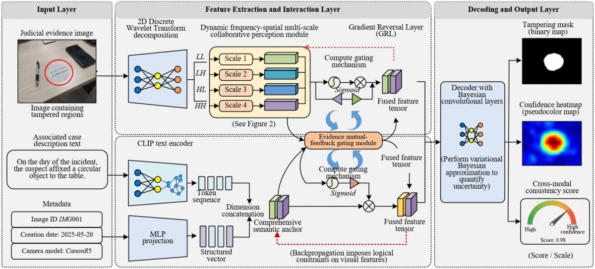
Figure 1 provides an overview of the unified framework for structure-semantic collaborative evidence reasoning.
Figure 1. Overview of the unified framework for structure-semantic collaborative evidence reasoning
Let the input judicial evidence image be $I \in \mathrm{R}^{3 \times H \times W}$, the associated case description text be $T$ (containing $L$ tokens), and the metadata be $M$. The goal of the framework is to output a triple evidentiary result: a pixel-wise tampering probability mask $\widehat{Y} \in[0,1]^{H \times W}$, a confidence heatmap $C \in[0,1]^{H \times W}$, and a cross-modal consistency score $\rho \in [0,1]$. To achieve this goal, the framework constructs a complete forward path from visual encoding to semantic alignment and finally to uncertainty decoding. Its core design principle is to enable visual representations and semantic logic to mutually constrain each other through iterative interaction.
In the visual encoding stage, image $I$ is decomposed via a 2D discrete wavelet transform into a low-frequency approximation component and three high-frequency detail components. After channel dimension upscaling on each frequency band, the features are fed into $K=4$ scales of DSPUs. By extending deformable convolution, this unit learns spatial offsets, scale modulation factors, and amplitude gating for each sampling point, allowing the receptive field to adaptively adjust according to the scale characteristics of tampered regions. Subsequently, a CSFA module computes a non-rigid offset field to accurately warp high-level semantic features onto the spatial grid of low-level features. After bidirectional propagation (top-down and bottom-up), the visual evidence tensor $V \in \mathrm{R}^{C_v \times H \times W}$ is output, where $C_v=256$. In the semantic encoding branch, the text $T$ is mapped to a token sequence $\left(T \in \mathrm{R}^{L \times C_t}, C_t=512\right)$ via a frozen CLIP text encoder. The metadata $M$ is projected into a structured vector $M \in \mathrm{R}^{C_m}$ via a multi-layer perceptron and concatenated with $T$ along the sequence dimension to form a comprehensive semantic anchor $S \in \mathrm{R}^{(L+1) \times C_t}$.
The key to achieving a visual-semantic bidirectional closed loop lies in the evidence mutual-feedback gating module. This module computes the gating matrices from vision to semantics and from semantics to vision, respectively:
$G_{v \rightarrow s}=\sigma\left(\operatorname{Conv}_{1 \times 1}(V) \otimes S^{\top}\right), G_{s \rightarrow v}=\sigma\left(S \otimes\right.$ Flatten $\left.(V)^{\top}\right)$ (1)
where, $\sigma$ is the Sigmoid function, $\otimes$ denotes batch matrix multiplication, and $\operatorname{Conv}_{1 \times 1}$ compresses the channels of the visual tensor to match the semantic space dimension. $G_{v \rightarrow s} \in \mathrm{R}^{H W \times(L+1)}$ maps salient visual regions to the semantic space to enhance the response of relevant textual features, while $G_{s \rightarrow v} \in \mathrm{R}^{(L+1) \times H W}$ utilizes textual logic constraints to generate a spatial attention mask that suppresses visual noise. The fused feature tensor $F_{\text {fus}}$ is obtained via a residual connection:
$F_{\text {fus}}=V \oplus U p$ Sample $\left(G_{s \rightarrow v} \odot S_{\text {proj}}\right)$ (2)
where, $S_{\text {proj}} \in \mathrm{R}^{C_v \times H \times W}$ is the result of projecting semantic features into the visual space, ⊙ denotes element-wise weighting, and $\oplus$ denotes additive fusion. This design ensures that during backpropagation, the visual feature extractor not only receives gradients from the segmentation loss but also receives constraints from the contrastive loss via a GRL. The forward propagation remains an identity mapping, while during backpropagation, the gradient is multiplied by $-\lambda_{g r l}$, forcing the visual encoder to discard responses irrelevant to the textual logic. The fused feature $F_{\text {fus}}$ is fed into a decoder equipped with Bayesian convolutional layers. Through multiple Monte Carlo stochastic forward passes, the mean and variance of the tampering probability are output, which are then used to generate the aforementioned triple evidentiary outputs, providing actionable trustworthiness grounds for subsequent judicial evidence examination.
2.2 Dynamic frequency-spatial multi-scale collaborative perception mechanism
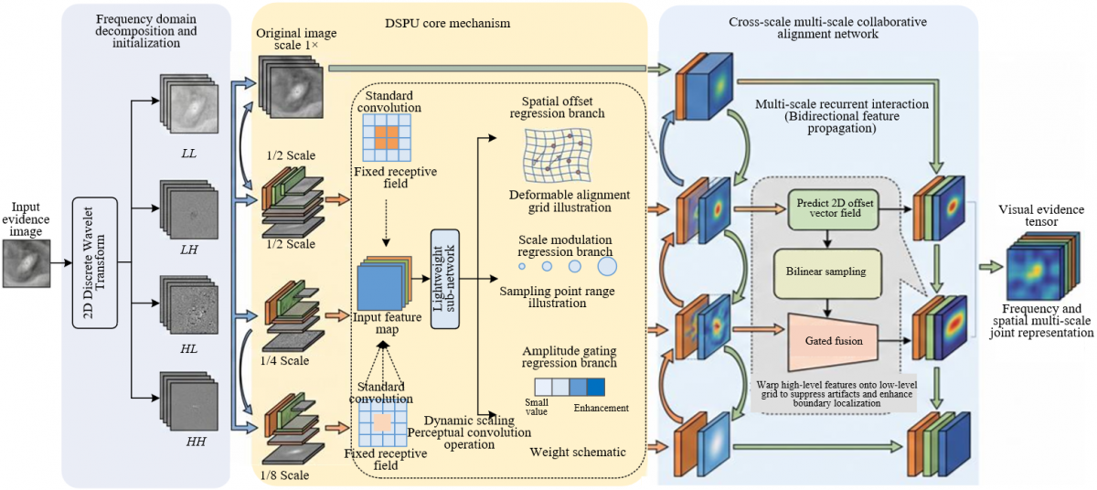
Traces of image tampering exhibit distinct distribution characteristics in the spatial and frequency domains: splicing operations often leave semantic inconsistencies in low-frequency approximation components, while copy-move or inpainting retouching exposes textural anomalies in high-frequency detail components. Single-scale spatial cues struggle to simultaneously cover large-scale structural dissonance and minute edge discontinuities; thus, multi-scale frequency-spatial joint perception becomes an intrinsic requirement for tampering localization. However, simply upsampling and adding multi-scale feature maps suffers from significant drawbacks: on one hand, geometric misalignment exists between different scale features, and direct fusion introduces artifacts and blurs tampering boundaries; on the other hand, shallow high-resolution features are rich in spatial details but lack semantic selectivity, while deep low-resolution features encode semantic information but lose spatial precision. The effective fusion of their complementary information necessitates a dynamic mechanism capable of simultaneously coordinating receptive fields, spatial positions, and feature magnitudes. To this end, this paper constructs a collaborative perception pipeline comprising three progressive components: frequency domain decomposition and initialization, DSPUs, and a CSFA module. Figure 2 illustrates the network structure of the dynamic frequency-spatial multi-scale collaborative perception mechanism.
Figure 2. Network structure of the dynamic frequency-spatial multi-scale collaborative perception mechanism
The input image is decomposed via a 2D discrete wavelet transform into a lowfrequency approximation component $F_{L L}$ and three high-frequency detail components $F_{L H}, F_{H L}$, and $F_{H H}$, where the high-frequency components correspond to edge and texture information in the horizontal, vertical, and diagonal directions, respectively. Compared to direct downsampling in RGB space, frequency domain decomposition offers the advantage of separating image content from noise textures into different subbands, enabling the subsequent network to specifically learn tampering artifact patterns on different frequency bands. After applying independent convolutional layers for channel upscaling on each frequency band, an initial multi-scale feature group $\left\{X^0, X^1, X^2, X^3\right\}$ is constructed, corresponding to the original scale, half scale, quarter scale, and one-eighth scale, respectively. The rationale for maintaining four progressive scales is that the relative size span of tampered objects within an image is vast: largearea spliced objects require a large-scale receptive field to capture their semantic inconsistency, while fine inpainting boundaries often manifest only as weak phase anomalies in the high-frequency sub-bands at the one-eighth scale.
DSPU extends the modeling capability of deformable convolution. Standard deformable convolution learns spatial offsets $\Delta p_k$ for each sampling point to adapt the convolution kernel shape to target geometric variations, but the contribution weight of each sampling point is fixed and cannot be dynamically adjusted based on local scale features of the tampering. This unit additionally introduces two learnable factors: a scale modulation factor $\Delta m_k \in(0,1)$ and an amplitude gate $\Delta a_k \in(0,2)$. For the feature map $X^s$ at the $s$-th scale, the convolution response at output position $p$ is defined as:
$Y^s(p)=\sum_{k=1}^K w_k \cdot X^s\left(p+p_k+\Delta p_k\right) \cdot \Delta m_k \cdot \Delta a_k$ (3)
where, $K$ is the total number of convolution kernel sampling points, $w_k$ is the fixed convolution weight, and $p_k$ is the preset offset of the $k$-th sampling point. The offset $\Delta p_k$, modulation factor $\Delta m_k$, and amplitude gate $\Delta a_k$ are all dynamically regressed by a lightweight sub-network $\Phi$ from the channel concatenation of the current scale feature $X^s$ and the upsampled feature $U\left(X^{s+1}\right)$ from the adjacent scale. The physical interpretation of this design is clear: large-area splicing tampering requires a larger receptive field, in which case the sub-network tends to output larger $\Delta p_k$ and an amplitude gate greater than 1 to enhance the response; conversely, minute textural tampering requires a narrow receptive field and high-frequency suppression, corresponding to smaller offsets and amplitude modulation less than 1. It is worth noting that $\Delta m_k$ and $\Delta a_k$ are decoupled during training; the former controls the effective contribution range of the sampling point, while the latter adjusts the overall scaling of the feature magnitude. Together, they enable the convolution kernel to adaptively adjust its geometric structure and response intensity according to the spatial scale characteristics of the tampered region.
The CSFA module aims to resolve the geometric misalignment between feature maps of different scales. Directly upsampling high-level features and adding them to low-level features blurs tampering boundaries due to spatial misalignment. Particularly when tampered regions have irregular shapes, artifacts introduced by simple addition severely impact boundary localization accuracy. This module introduces a non-rigid alignment field, predicting a 2D offset vector $\delta(p) \in \mathrm{R}^2$ for each target position $p$ on the current layer feature map, allowing the high-level semantic feature $F^{l+1}$ to be precisely warped onto the spatial grid of the low-level feature $F^l$. The offset is implicitly learned by maximizing local cross-correlation, and the forward warping operation employs a differentiable bilinear sampling mechanism:
$F_{\text {warp}}^{l+1}(p)=\sum_{q \in N(p+\delta(p))} F^{l+1}(q) \cdot \max \left(0,1-\left|p_x+\delta_x(p)-q_x\right|\right) \cdot \max \left(0,1-\left|p_y+\delta_y(p)-q_y\right|\right)$ (4)
where, $N(p+\delta(p))$ denotes the neighborhood grid centered at the offset position, $q_x$ and $q_y$ are the spatial coordinates of the sampling points within the neighborhood. This equation essentially performs linear interpolation based on the sub-pixel distance between the offset position and the neighborhood grid points, allowing gradients to be backpropagated through $\delta(p)$ to the offset prediction sub-network, thereby enabling end-to-end learning. After feature alignment, a gated fusion strategy is adopted to update the current layer representation:
$F_{\text {align}}^l=\operatorname{Conv}\left(\left[F^l, F_{\text {warp}}^{l+1}\right]\right) \odot \sigma\left(\operatorname{Conv}_{\text {gate}}\left(\left[F^l, F_{\text {warp}}^{l+1}\right]\right)\right)$ (5)
where, [ , ] denotes channel concatenation, $\sigma$ is the Sigmoid function, $Conv_{gate}$ outputs a spatial gating mask with a single channel, and ⊙ denotes element-wise multiplication. This gating mechanism allows the network to adaptively determine the fusion intensity at each spatial position based on alignment quality: the gating value approaches 1 where alignment is reliable, and approaches 0 where alignment is unreliable.
After completing two iterations each of top-down and bottom-up bidirectional propagation, the features across the four scales gradually converge to a shared spatial coordinate system through the alignment and fusion processes. The final output visual evidence tensor $V \in \mathrm{R}^{C_v \times H \times W}$ encodes a multi-scale joint representation of both low-frequency semantic consistency and high-frequency textural anomalies along the channel dimension, providing an information-complete visual foundation for subsequent cross-modal semantic alignment and uncertainty decoding.
2.3 Cross-modal evidence consistency verification module
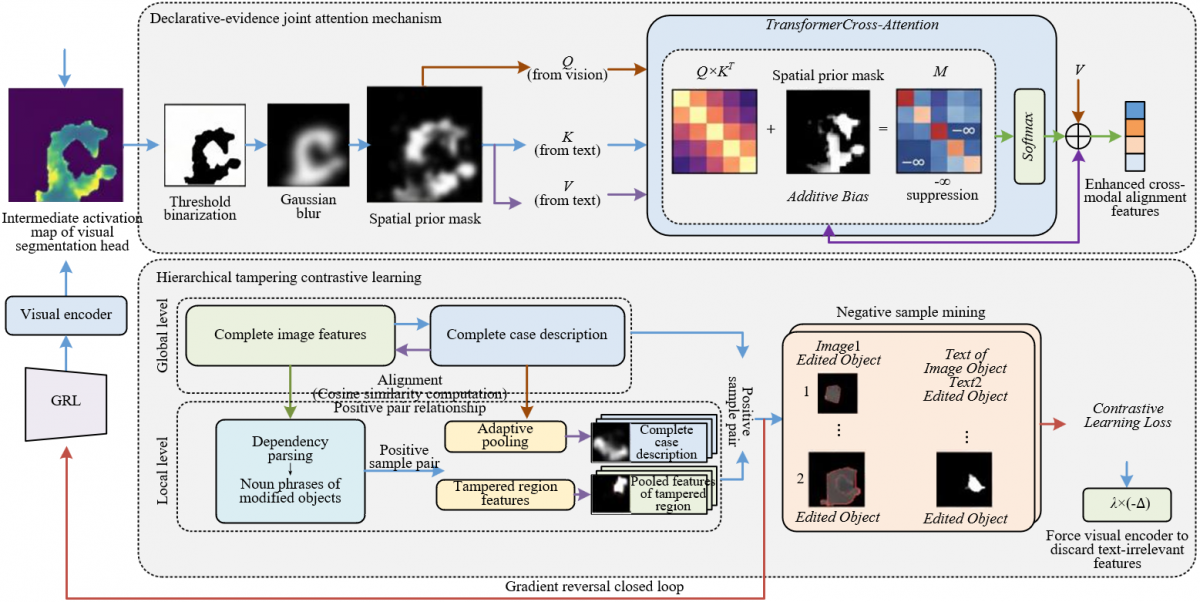
A tampering localization mask can only answer where an image has been modified, whereas the core requirement in judicial forensics lies in determining whether the tampered content is compatible with the factual case description. The key challenge in this cross-modal verification task is the alignment gap between the representation spaces of visual localization results and textual semantic descriptions: visual features encode pixel-level texture and structural information, while textual features encode abstract concepts and relational descriptions. Their alignment requires not only spatial correspondence at the perceptual level but also logical matching at the semantic level. To this end, this paper constructs a cross-modal verification module indexed by visual anchors, comprising three collaborative components: declarative-evidence joint attention, hierarchical tampering contrastive learning, and gradient reversal closed-loop feedback. This design aims to mutually constrain visual representations and semantic logic within a unified latent space, ultimately outputting a quantifiable evidence consistency score. Figure 3 illustrates the principle of the cross-modal evidence consistency verification module.
Figure 3. Schematic diagram of the cross-modal evidence consistency verification module
The core design of the declarative-evidence joint attention mechanism lies in utilizing the spatial prior mask provided by intermediate layers of the tampering localization head to guide the focusing process of textual features within the visual space. Let the intermediate activation map from the visual segmentation head be thresholded into a binary mask and then smoothed via Gaussian blur to generate the spatial prior mask $M_{g e o} \in[0,1]^{H \times W}$. This mask reflects the model's current pixel-wise confidence regarding whether a specific location belongs to a tampered region. During cross-modal attention computation, this mask is injected as an additive bias into the dot-product similarity between the query and key:
$Attn_{\text {cross}}=\operatorname{Softmax}\left(\frac{Q \cdot T^{\top}}{\sqrt{d}}+\log \left(M_{\text {geo}}+\epsilon\right)\right)$ (6)
where, $Q \in \mathrm{R}^{H W \times d}$ is the query matrix obtained by linearly projecting the visual features, $T \in \mathrm{R}^{L \times d}$ is the key matrix obtained by linearly projecting the textual token sequence, $d$ is the dimension of the attention head, and $\epsilon=10^{-8}$ is a constant to prevent the logarithm from approaching negative infinity. The additive bias term $\log \left(M_{\text {geo}}+\epsilon\right)$ transforms the spatial prior into a multiplicative modulation of the attention weights: when a location is classified as a high-suspicion region, the bias term approaches 0, and the attention weight is primarily driven by visual-semantic similarity; when a location is classified as a low-suspicion region, the bias term approaches negative infinity, and the corresponding attention weight is forcibly suppressed. This design enables the text encoder to focus its limited computational resources on semantic descriptions related to tampered regions, rather than distributing them uniformly across all spatial positions of the entire image.
Hierarchical tampering contrastive learning establishes multi-level semantic alignment constraints ranging from the global scene to local objects, addressing the need for evidence consistency discrimination at different granularities. The global level uses the matching of complete image features with the full case description as a basic constraint to ensure overall semantic consistency. The local level utilizes dependency parsing to extract noun phrases describing the modified object from the case description, forming positive sample pairs with the pooled features of the corresponding tampered regions in the visual branch. In cross-level hard negative mining, the tampered region feature of one sample within the same batch and the irrelevant description of another sample constitute a strong negative pair. The dynamic hard example mining loss for the latter is defined as:
$L_{\text {hard}}=-\frac{1}{B} \sum_{i=1}^B \log \frac{\exp \left(\operatorname{sim}\left(v_i^{\text {tam}}, t_i^{\text {desc}}\right) / \tau\right)}{\exp \left(\operatorname{sim}\left(v_i^{\text {tam}}, t_i^{\text {desc}}\right) / \tau\right)+\sum_{j \in H_i} \exp \left(\operatorname{sim}\left(v_i^{\text {tam}}, t_j^{\text {desc}}\right) / \tau\right)}$ (7)
where, $B$ is the batch size, $v_i^{\text {tam}} \in \mathrm{R}^{C_v}$ is the global feature of the tampered region of the $i$-th sample after adaptive pooling, $t_i^{\text {desc}} \in \mathrm{R}^{C_t}$ is the feature of the phrase corresponding to the tampered object in the case description after encoding by the text encoder, sim( , ) denotes cosine similarity, and $\tau$ is a temperature hyperparameter. $H_i$ is the set of indices for negative samples whose feature similarity to sample $i$ ranks in the top $K_{\text {hard}}$. This dynamic screening strategy forces the model to not only distinguish explicitly different sample pairs but also focus on hard samples with ambiguous semantic boundaries, thereby learning more discriminative cross-modal alignment representations.
GRL acts as a bidirectional information gate between the visual encoder and the semantic encoder, serving as the core hub for achieving closed-loop optimization between localization and verification. During forward propagation, the GRL performs an identity mapping, allowing semantic and visual features to interact seamlessly in attention computations. During backpropagation, however, it multiplies the gradient of the contrastive loss $L_{\text {contra}}$ with respect to the semantic branch parameter $\theta_{\text {sem}}$ by a negative coefficient before passing it to the visual branch parameter $\theta_{\text {vis}}$, specifically:
$\frac{\partial L_{\text {contra}}}{\partial \theta_{\text {vis}}}=-\lambda_{\text {grl}} \cdot \frac{\partial L_{\text {contra}}}{\partial \theta_{\text {sem}}}, \lambda_{\text {grl}}(t)=\min \left(0.1,0.1 \cdot t / T_{\text {warmup}}\right)$ (8)
where, $\lambda_{g r l}$ is the reversal strength coefficient, which linearly increases from 0 to 0.1 during the warmup phase and then remains constant. This gradient reversal operation subjects the visual feature extractor to adversarial constraints from the semantic branch: if the visual features contain spurious responses irrelevant to the case description, the gradient generated by the cross-modal contrastive loss in the semantic branch, after reversal, will act in the direction of increasing the response intensity in the visual branch, thereby increasing the total loss. This forces the visual encoder to gradually discard feature responses unrelated to the textual logic. Together, these three components form a co-evolution mechanism where localization serves verification and verification feeds back to localization, allowing tampering localization and cross-modal verification to mutually promote each other during joint training.
2.4 Boundary-aware uncertainty learning and interpretable output
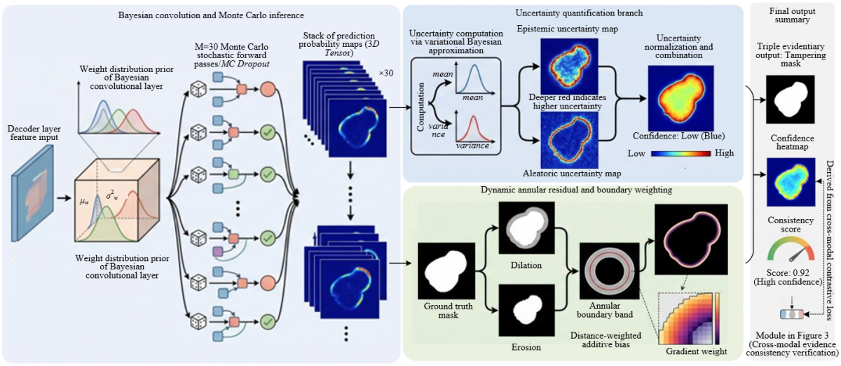
In judicial forensics scenarios, if the prediction results of a deep learning model are presented merely as binary masks without quantitative explanations of the model’s own judgment reliability, they are difficult to admit as valid forensic support. Forensic examiners require not only the spatial location of tampered regions but also a clear understanding of the model’s prediction confidence for those regions and the geometric accuracy of boundary localization. To this end, this paper introduces variational Bayesian approximation in the decoding stage to quantify predictive uncertainty, designs boundary-aware loss constraints to enhance the localization accuracy of tampered region boundaries, and ultimately generates a triple output comprising a tampering mask, a confidence heatmap, and a consistency score. Figure 4 illustrates the schematic of uncertainty decoding and boundary-aware output.
Figure 4. Schematic of uncertainty decoding and boundary-aware output
Bayesian convolutional layers are adopted in the last three convolutional layers of the decoder, imposing a Gaussian prior $w \sim N\left(0, \sigma_p^2 I\right)$ on the weight parameters, where, $\sigma_p^2$ is the hyperprior variance used to control the scale of the prior weight distribution. Since exact inference of the Bayesian posterior in deep networks is computationally intractable, this paper employs Monte Carlo dropout approximation as a surrogate for variational inference: during forward propagation, neuron outputs are randomly set to zero with a dropout rate $p_{\text {drop}}=0.3$. In the variational framework, this operation is equivalent to searching for an approximate distribution within the Bernoulli distribution family that minimizes the Kullback-Leibler (KL) divergence from the true posterior. After performing $M=30$ stochastic forward passes, the prediction distribution $\left\{\hat{y}_i^{(m)}\right\}_{m=1}^M$ is obtained for each pixel. Based on this distribution, epistemic uncertainty and aleatoric uncertainty can be computed respectively:
$U n c_{e p i}(i)=\frac{1}{M} \sum_{m=1}^M\left(\hat{y}_i^{(m)}-\bar{y}_i\right)^2, \bar{y}_i=\frac{1}{M} \sum_{m=1}^M \hat{y}_i^{(m)}$ (9)
$\operatorname{Unc}_{\text {ale}}(i)=\frac{1}{M} \sum_{m=1}^M \hat{y}_i^{(m)}\left(1-\hat{y}_i^{(m)}\right)$ (10)
where, epistemic uncertainty $U_{n c_{\text {epi}}}(i)$ measures the dispersion of prediction results across multiple samplings, reflecting the model's lack of knowledge regarding the classification decision for that pixel. Aleatoric uncertainty $U n c_{\text {ale}}(i)$ measures the fuzziness of the classification boundary in a single prediction, reflecting inherent noise or ambiguity in the input data. The final confidence heatmap is defined as $C_i=1$ -$U n c_{\text {epi}}(i)-U n c_{\text {ale}}(i)$, with a value range of [0,1]. Higher values indicate greater certainty in the model's prediction of the pixel's tampering probability. This design enables forensic examiners to intuitively identify regions of high prediction reliability and ambiguous regions requiring manual review.
The localization accuracy of tampered region boundaries directly impacts the quality of spatial references for evidence consistency verification. Significant boundary prediction offsets reduce the reliability of the overall tampered region localization. This paper proposes a dynamic annular residual module to impose additional structured supervision on tampering boundaries during training. Given the ground truth mask $Y$, dilation and erosion operations are sequentially applied with a dilation kernel radius and an erosion kernel radius $r_{\text {dil}}=5$, respectively, to extract the annular boundary band $r_{\text {ero}}=3$. Pixels within this boundary band $B=$ Dilate $(Y) \backslash \operatorname{Erode}(Y)$ correspond to the outer transition zone of the tampered region, representing the area most prone to classification errors. To assign differentiated gradient intensities to pixels at different positions within the boundary band, a distance-weighted loss is defined as follows:
$L_{\text {boundary}}=\frac{1}{|B|} \sum_{i \in B} L_{B C E}\left(\hat{y}_i, y_i\right) \cdot\left(1+\alpha \cdot e^{-\beta d_i}\right)$ (11)
where, $L_{B C E}$ is the binary cross-entropy loss, $d_i$ is the Euclidean distance from pixel $i$ to the nearest internal tampered pixel, normalized to [0,1], and $\alpha=2.0$ and $\beta=0.5$ are hyperparameters controlling the weight decay rate. This weighting strategy assigns approximately three times the loss weight to pixels immediately adjacent to the outer edge of the tampered region $\left(d_i \rightarrow 0\right)$, forcing the model to prioritize optimizing these boundary decisions during backpropagation, thereby effectively suppressing boundary localization offsets.
The total training loss function comprises three components: segmentation loss, cross-modal contrastive loss, and uncertainty loss:
$L_{\text {total}}=\lambda_1 L_{\text {seg}}+\lambda_2 L_{\text {contra}}+\lambda_3 L_{\text {unc}}$ (12)
where, $L_{\text {seg}}$ includes Dice loss, Focal loss, and the aforementioned boundary-weighted loss, supervising the pixel-level tampering localization accuracy. $L_{\text {contra}}$ is the cross-modal contrastive loss, constraining the consistency between visual representations and semantic logic. $L_{\text {unc}}$ is the uncertainty regularization term, computed from the KL divergence between the Bayesian convolutional layer weight prior and the variational posterior. The hyperparameters are set as $\lambda_1=1.0, \lambda_2=0.8$, and $\lambda_3=0.3$. It is worth noting that $L_{\text {unc}}$ may cause gradient oscillation in the early stages of training; therefore, a KL annealing strategy is introduced, multiplying it by a dynamic weight $\eta(t)=\min \left(1.0, t / t_{\text {warmup}}\right)$, where $t$ is the current iteration step and $t_{\text {warmup}}=5000$. This strategy gradually integrates the uncertainty loss into the total loss during the first 5,000 iterations, preventing overly strong prior constraints from prematurely dominating the optimization direction before features have sufficiently converged. After the aforementioned joint training, the decoder outputs a triple evidentiary result during inference: the pixel-wise tampering probability mask $\widehat{Y}$, the confidence heatmap $C$, and the global consistency score $\rho$ derived from the cross-modal contrastive loss. This provides forensic examiners with actionable decision support that combines spatial precision with confidence references.
2.5 Joint optimization objective and training strategy
The collaborative operation of the aforementioned components relies on a joint optimization objective that must simultaneously account for pixel-level segmentation accuracy, cross-modal semantic consistency, and the reliable calibration of prediction confidence. The total loss function is defined as a weighted sum of four loss components:
$L_{\text {total}}=\lambda_1 L_{\text {seg}}+\lambda_2 L_{\text {contra}}+\lambda_3 L_{\text {unc}}+\lambda_4 L_{\text {hard}}$ (13)
where, $L_{\text {seg}}$ is the segmentation loss, supervising the pixel-level accuracy of tampering localization. $L_{\text {contra}}$ is the global cross-modal contrastive loss, constraining the semantic alignment between overall image features and the case description. $L_{\text {unc}}$ is the uncertainty regularization term, computed from the KL divergence between the weight prior and the variational posterior in the Bayesian convolutional layers, serving to prevent the model from overconfidently outputting erroneous predictions. $L_{\text {hard}}$ is the dynamic hard example mining loss, imposing additional contrastive constraints on cross-level negative sample pairs. The hyperparameters for each loss component are tuned based on validation set performance and set as $\lambda_1=1.0, \lambda_2=0.8, \lambda_3=0.3$, and $\lambda_4=0.5$. Here, $\lambda_1$ is set as the baseline weight to maintain the dominant role of the segmentation task; $\lambda_2$ and $\lambda_4$ jointly control the strength of cross-modal alignment; while $\lambda_3$ is assigned a smaller value to prevent the uncertainty regularizer from excessively interfering with the learning of the main task.
The segmentation loss $L_{\text {seg}}$ is further decomposed into the sum of three terms:
$L_{\text {seg}}=L_{\text {Dice}}+L_{\text {Focal}}+L_{\text {boundary}}$ (14)
Among these, the Dice loss mitigates the class imbalance between tampered regions and the background. The Focal loss reduces the weight of easy-to-classify samples, forcing the model to focus on discriminating hard samples. The boundary loss $L_{\text {boundary}}$ applies distance-weighted supervision to pixels within the outer transition band of the tampered region. It is worth noting that $L_{\text {boundary}}$ participates only in gradient backpropagation during the training phase; its computation relies on morphological boundary extraction from the ground truth mask. This module is entirely removed during inference and thus incurs no additional computational overhead during deployment.
Training adopts a two-stage strategy to balance the convergence rates of visual feature learning and cross-modal semantic alignment. In the first stage, the CLIP text encoder is frozen, and only the parameters of the visual branch and the decoder are optimized for 50 epochs. The objective of this stage is to endow the visual feature extractor with robust tampering localization capabilities, preventing unoptimized visual features from propagating noisy gradients to the semantic branch. In the second stage, all network parameters are unfrozen for end-to-end fine-tuning over another 50 epochs, during which the strength coefficient $\lambda_{g r l}$ of the GRL linearly increases from 0 to 0.1 . This warmup scheduling strategy allows the visual branch to prioritize optimization for the segmentation task in the early stages, while gradually intensifying adversarial constraints from the semantic branch as training progresses, thereby achieving a smooth transition between localization accuracy and semantic consistency. The entire training process utilizes the AdamW optimizer with an initial learning rate of $1 \times 10^{-4}$, which decays $1 \times 10^{-6}$ to over the training cycle via a cosine annealing strategy. The batch size is set to 16 .
3.1 Experimental setup
The experiments cover five public benchmark datasets and one self-constructed dataset. CASIA v2.0 contains 7,491 images involving splicing and copy-move tampering. NIST16 provides diverse tampering types and post-processing operations, comprising 564 images. IMD 2020 covers three tampering types—splicing, copy-move, and removal—with a total of 2,101 images. Defacto focuses on image tampering in real-world scenarios and contains 3,500 images. Columbia provides uncompressed spliced images, totaling 363 images. The self-constructed Forensic Evidence Set (FES) contains 1,200 case-related images, each accompanied by detailed case description text, timestamps, and geolocation metadata. It covers four tampering types: splicing, copy-move, removal inpainting, and AI-generated semantic replacement. All datasets are partitioned into training, validation, and test sets at a ratio of 6:2:2. The specific scales are detailed in Table 1.
For pixel-level tampering localization, F1-score, Intersection over Union (IoU), and the Area Under the Receiver Operating Characteristic Curve (AUC) are adopted as evaluation metrics. For cross-modal verification, cross-modal consistency accuracy is used, defined as the proportion of samples where the model correctly identifies inconsistency between the tampered region and the text description, as confirmed by manual annotation. The evidence trustworthiness score is defined as $1-1 / \mathrm{N} \sum_{i=1}^N\left|\hat{y}_i-y_i\right| \cdot U n c_{e p i}(i)$. This score simultaneously considers localization accuracy and prediction confidence, with a value range of $[0,1]$; higher values indicate stronger evidence reliability.
Implementation details are as follows. All experiments are conducted on an NVIDIA A100 GPU using the PyTorch framework. The visual backbone is ImageNet pre-trained EfficientNet-B4. In the DSPU, the deformable convolution kernel size is set to $3 \times 3$, with a total sampling point count $K=9$. The AdamW optimizer is employed with parameters $\beta_1=0.9$ and $\beta_2=0.999$. The initial learning rate is set to $1 \times 10^{-4}$ and decays to $1 \times 10^{-6}$ using a cosine annealing strategy. The batch size is 16, and the total training epoch count is 100 . The Monte Carlo dropout sampling count is $M=30$. All comparative methods are retrained on the training sets of respective datasets under their officially recommended parameter configurations and evaluated on the corresponding test sets.
Table 1. Statistics of dataset partitioning
|
Dataset |
Tampering Type |
Training Set |
Validation Set |
Test Set |
Total |
|
CASIA v2.0 |
Splicing / Copy-move |
4495 |
1498 |
1498 |
7491 |
|
NIST16 |
Multiple types |
338 |
113 |
113 |
564 |
|
IMD 2020 |
Splicing / Copy-move / Removal |
1260 |
421 |
420 |
2101 |
|
Defacto |
Real-world tampering |
2100 |
700 |
700 |
3500 |
|
Columbia |
Splicing (Uncompressed) |
218 |
72 |
73 |
363 |
|
Forensic Evidence Set (FES, Ours) |
Judicial scenario mix |
720 |
240 |
240 |
1200 |
3.2 In-domain performance comparison
S³ER is compared against six state-of-the-art methods on five public datasets: CAT-Net, MVSS-Net, PSCC-Net, DFFormer, HFZI, and UFG-Net. Table 2 reports the average and standard deviation of each method across three metrics: F1-score, IoU, and AUC.
Table 2. In-domain performance comparison of various methods on public datasets (Mean ± Standard deviation)
|
Method |
F1 (%) |
IoU (%) |
AUC (%) |
|
CAT-Net |
77.3 ± 1.2 |
63.1 ± 1.5 |
81.5 ± 1.1 |
|
MVSS-Net |
79.8 ± 1.0 |
66.4 ± 1.3 |
83.7 ± 0.9 |
|
PSCC-Net |
80.5 ± 0.9 |
67.2 ± 1.1 |
84.2 ± 0.8 |
|
DFFormer |
82.1 ± 0.8 |
69.8 ± 1.0 |
86.0 ± 0.7 |
|
HFZI |
83.4 ± 0.7 |
71.5 ± 0.9 |
87.3 ± 0.6 |
|
UFG-Net |
84.0 ± 0.7 |
72.3 ± 0.8 |
88.1 ± 0.6 |
|
S³ER(Ours) |
87.6 ± 0.5 |
76.8 ± 0.6 |
91.2 ± 0.4 |
Note: IoU = Intersection over Union; AUC = Area Under the Receiver Operating Characteristic Curve.
S³ER achieves optimal results across all three metrics. Compared to the second-best method, UFG-Net, S³ER improves the F1-score by 3.6%, IoU by 4.5%, and AUC by 3.1%. Notably, the standard deviation of S³ER is significantly smaller than that of all comparative methods; the F1 standard deviation is only 0.5, whereas those of UFG-Net and HFZI are 0.7 and 0.7, respectively. These results indicate that the proposed method exhibits more stable detection capabilities across different data distributions, effectively suppressing performance fluctuations. This advantage primarily stems from the adaptive fusion capability of the CSFA module via non-rigid offset fields for tampering traces at different scales. CASIA v2.0 is dominated by coarse-grained splicing, while Columbia focuses on fine-grained boundary tampering. The dynamic alignment mechanism of CSFA enables the model to maintain high precision on both types of data, avoiding the performance oscillations caused by the scale bias of traditional methods.
3.3 Cross-domain generalization performance
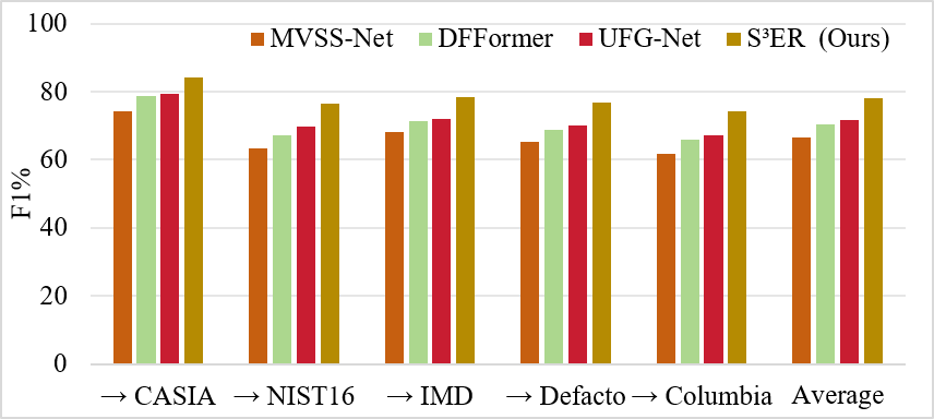
To evaluate the model's generalization capability on unseen datasets, a leave-one-dataset-out validation strategy is adopted: training is performed on four of the five public datasets, and testing is conducted on the remaining one. Figure 5 reports the comparative results for the F1-score.
Figure 5. Cross-domain generalization performance comparison (F1 %)
S³ER achieves an average F1-score of 78.0% in cross-domain scenarios, representing a 6.3% improvement over UFG-Net and a 7.6% improvement over DFFormer. The proposed method maintains a significant advantage across all target datasets, with the most prominent gain observed on NIST16, exceeding UFG-Net by 6.7%. Particularly noteworthy is the performance on the Columbia dataset, which consists of uncompressed, high-resolution images with a data distribution significantly different from the training sets. Under this setting, S³ER still achieves an F1-score of 74.2%, while all comparative methods score below 68%. This gain can be attributed to the scale modulation factors and amplitude gates learned by the DSPU, which adaptively adjust the convolutional receptive field and response intensity based on the scale characteristics of tampered regions. This allows the frequency-spatial collaborative patterns learned by the model on the training sets to be effectively transferred to unseen data with different compression attributes and resolution characteristics. These results fully validate the practical potential of the proposed method for real-world judicial scenarios involving diverse evidence sources.
3.4 Ablation analysis of core modules
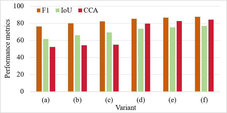
To quantify the independent contribution of each innovative component, six ablation variants are constructed on a mixed test set combining CASIA and FES. To systematically evaluate the effectiveness of the core modules, we design six progressive ablation variants (see Figure 6). Variant (a) serves as the baseline model, utilizing a standard multi-scale backbone network to extract visual features without introducing any frequency domain information or cross-modal interaction modules, thereby establishing a reference for measuring the incremental contributions of subsequent improvements. Variant (b) incorporates the DSPU into (a), enabling the network to adaptively adjust the receptive field range of the convolution kernels based on the input content, thereby enhancing the capture of tampering cues at different scales. Variant (c) further introduces the CSFA module, which employs learnable alignment mapping and bilinear interpolation to effectively mitigate semantic misalignment and spatial mismatch between multi-scale feature maps, ensuring the accuracy of cross-layer information fusion. Variant (d) builds upon the alignment by adding the declarative-evidence joint attention mechanism to capture fine-grained associations between different modalities and feature layers. This is supplemented by a hierarchical contrastive learning strategy that simultaneously pulls together representations of the same class and pushes apart those of different classes at both the sample and category levels, thereby strengthening the clustering of discriminative semantic prototypes. Variant (e) introduces the GRL, which backpropagates domain discrimination loss via an adversarial training strategy to suppress the confounding interference of low-level visual characteristics (such as lighting and texture) on semantic representation, forcing the network to focus on essential semantic features. Variant (f) integrates dynamic annular residual connections and an uncertainty-aware module into (e): the former promotes iterative optimization between deep and shallow features through a ring-topology structure to prevent information attenuation in deep networks, while the latter explicitly models prediction confidence using a heteroscedastic Gaussian distribution to quantify the predictive uncertainty of each sample. This constitutes the complete proposed model, namely EMO-Community Net.
Figure 6. Ablation study of core modules (F1 / IoU / CCA %)
From variants (a) to (b), the introduction of the DSPU yields a 3.6% increase in F1-score, indicating that dynamic receptive field adjustment is more effective at capturing multi-scale tampering traces compared to fixed-scale convolutions. Adding CSFA further increases the F1-score by 2.5%, confirming the necessity of precise alignment of multi-scale features via non-rigid offset fields. The most significant performance leap occurs in variant (d); upon introducing cross-modal verification, the F1-score rises by 2.8%, while the Cross-modal Consistency Accuracy (CCA) surges from 55.0% to 79.6%, an increase of 24.6%. This demonstrates that visual-textual semantic alignment substantially enhances the model's ability to discriminate semantic-level inconsistencies, a capability entirely absent in purely visual methods. In variant (e), the introduction of the GRL further increases the F1-score and CCA by 1.3% and 2.8%, respectively, confirming that the reverse constraints imposed by textual logic on visual features effectively eliminate false positive responses unrelated to semantics. The complete model achieves a CCA of 84.1% on the FES dataset, indicating that S³ER can provide forensic examiners with highly reliable semantic-level auxiliary adjudication.
3.5 Contribution analysis of loss function components
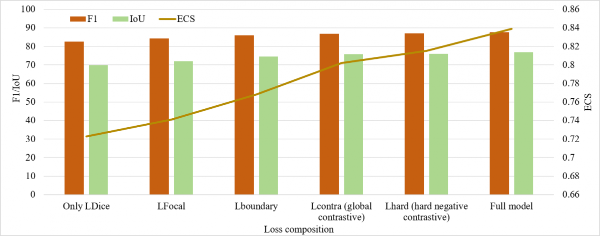
To verify the effectiveness of each component in the joint loss function, loss terms were progressively added while keeping the network architecture fixed. The results are shown in Figure 7.
The addition of Focal loss yields a 1.7% increase in F1-score compared to using Dice loss alone, indicating that the severe class imbalance between tampered regions and the background (where tampered areas typically occupy only 5% to 20% of an image) is effectively mitigated. The introduction of boundary loss contributes a further 1.7% improvement in F1-score, while simultaneously increasing the Evidence Credibility Score (ECS) by 0.027. This suggests that as uncertainty in boundary pixels is significantly reduced, the reliability of the overall evidence scoring is enhanced. Global contrastive loss improves the F1-score by 0.9%, while the gain from hard example loss is relatively marginal at 0.3%. This indicates that global-level visual-textual alignment is already capable of establishing strong semantic associations, with hard example mining providing only incremental improvements on this foundation. Although the addition of uncertainty loss yields only an extra 0.5% increase in F1-score, it significantly elevates the ECS from 0.815 to 0.839. This confirms that the Bayesian calibration layer effectively suppresses overconfident erroneous predictions, thereby markedly enhancing the reliability of evidence trustworthiness assessment while maintaining localization accuracy.
Figure 7. Ablation study of loss function components (F1 / IoU / ECS)
3.6 Robustness analysis
Judicial evidence images are frequently subjected to post-processing operations such as JPEG compression, noise contamination, and geometric transformations during acquisition, transmission, and storage. Various attacks of differing intensities were applied to the FES test set to compare the F1-score degradation of S³ER against UFG-Net and DFFormer. The results are presented in Table 3.
Table 3. Robustness comparison under different post-processing attacks (F1 %)
|
Attack Type |
Parameters |
UFG-Net |
DFFormer |
S³ER |
|
No Attack |
- |
84 |
82.1 |
87.6 |
|
JPEG Compression |
QF = 70 |
79.2 |
77.5 |
85.3 |
|
JPEG Compression |
QF = 30 |
72.4 |
70.1 |
81.6 |
|
Gaussian Blur |
σ = 1.5 σ = 1.5 |
76.8 |
75.2 |
82.9 |
|
Gaussian Noise |
σ = 0.05 σ = 0.05 |
73.5 |
70.9 |
80.4 |
|
Resizing |
0.5× + Bicubic interpolation |
78.1 |
75.8 |
83.7 |
|
Contrast Adjustment |
Gain = 1.8 |
80.3 |
78.9 |
85.6 |
Under no-attack conditions, S³ER achieves an F1-score of 87.6%, significantly higher than UFG-Net's 84.0%. When subjected to strong JPEG compression with a Quality Factor (QF) of 30, S³ER's F1-score drops to 81.6%, representing a decrease of 6.0%, whereas UFG-Net suffers a substantial drop of 11.6%. The strong robustness of S³ER against JPEG compression stems from the 2D discrete wavelet transform-based frequency domain decomposition strategy; the energy distribution of tampering traces in directional sub-bands is less affected by quantization tables. Furthermore, the CSFA module effectively resists compression interference by preserving high-frequency residual information. Under Gaussian noise attacks, the performance of all methods declines considerably; however, S³ER maintains an F1-score of 80.4%. This resilience is attributed to the uncertainty estimation layer, which effectively suppresses random noise-induced misclassifications during inference through averaging over multiple Monte Carlo sampling passes. Under resizing attacks, S³ER exhibits only a 3.9% drop, validating the adaptive capability of the DSPU to scale variations.
3.7 Cross-modal verification performance analysis
This experiment quantifies the effect of the cross-modal consistency verification module on different tampering types within the FES dataset. The CCA and ECS were compared with and without this module, and the results are presented in Table 4.
For AI-generated semantic replacement tampering, the CCA without the cross-modal module is only 48.9%, significantly lower than the 61.3% observed for traditional splicing tampering. This is because generative models can maintain extremely high visual consistency at the pixel level, leaving pure visual methods with almost no discernible clues; consequently, outputs frequently conflict with textual descriptions. With the introduction of cross-modal verification, the CCA for this category jumps to 78.4%, an increase of 29.5%. These results demonstrate that when visual cues are ambiguous, the declarative-evidence joint attention mechanism can leverage textual semantic information to make correct judgments. For instance, if the text describes a collision scratch on the left front fender, but the generated image shows a smooth texture in that region, the semantic contradiction becomes the key basis for determination. Regarding the ECS, the introduction of the cross-modal module increases the ECS for all tampering types by approximately 0.12. This indicates that semantic consistency constraints lead the model to output higher uncertainty rather than blind confidence when sufficient visual evidence is lacking. This characteristic holds significant methodological alignment with the judicial principle of in dubio pro reo (presumption of innocence when in doubt).
Table 4. Cross-modal verification performance under different tampering types (self-constructed Forensic Evidence Set (FES) Dataset)
|
Tampering Type |
Sample Count |
CCA (w/o Cross-Modal) |
CCA (w/ Cross-Modal) |
ECS (w/o Cross-Modal) |
ECS (w/ Cross-Modal) |
|
Splicing |
80 |
61.3 |
85.6 |
0.731 |
0.851 |
|
Copy-Move |
60 |
58.3 |
82.5 |
0.712 |
0.833 |
|
Removal Inpainting |
55 |
52.7 |
80.9 |
0.694 |
0.824 |
|
AI-Generated Semantic Replacement |
45 |
48.9 |
78.4 |
0.665 |
0.806 |
Note: FES = Forensic Evidence Set; CCA = Cross-modal Consistency Accuracy; ECS = Evidence Credibility Score.
3.8 Visualization analysis and discussion
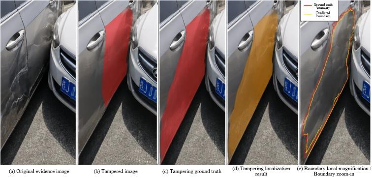
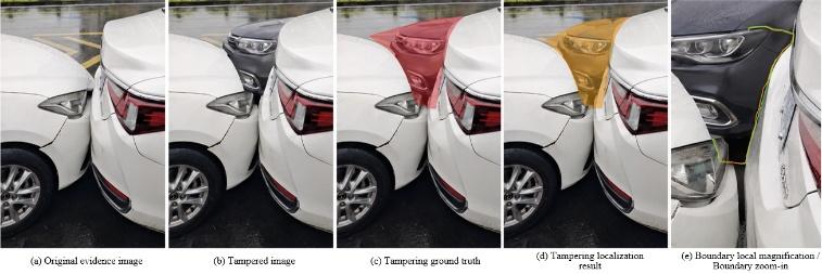
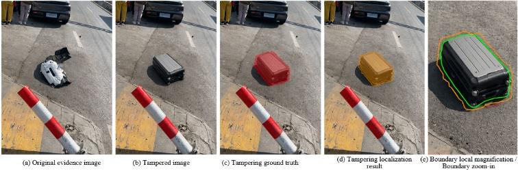
To verify the fine-grained localization capability of the proposed method against image tampering mechanisms in judicial digital evidence scenarios, and to examine whether it can provide stable and reliable visual evidence anchors for subsequent cross-modal consistency verification, visualization experiments were conducted on three representative samples: localized splicing tampering, removal inpainting tampering, and AI-generated semantic replacement. Figure 8(a) demonstrates that for localized splicing tampering, the model accurately focuses on the spliced region within a complex vehicle collision scene. The prediction results exhibit high spatial consistency with the ground truth masks. Local magnification of the boundaries further reveals that the model maintains good adherence to target contour turning points and contact edges. This suggests that the multi-scale frequency-spatial collaborative perception mechanism effectively identifies tampering traces formed by the combination of local structural mutations and textural dissonance. Figure 8(b) shows that in removal inpainting tampering, although significant visual mutations in the tampered region are diminished by content smoothing and texture reconstruction, the proposed method still stably recovers the overall extent of the tampered area and achieves localization results consistent with the ground truth in terms of boundary details. This indicates that the CSFA and boundary constraint mechanisms effectively enhance sensitivity to weak-trace inpainting tampering. Figure 8(c) further illustrates that in AI-generated semantic replacement scenarios, despite the tampered object possessing stronger visual naturalness and weaker traditional editing traces, the model accurately locks onto the semantic replacement target and generates a closed and clear boundary response. This confirms that the proposed method can not only identify explicit tampering but also establish stable localization for semantic anomalies in generative forgeries. Synthesizing the results from the three groups, it is evident that the proposed method exhibits strong localization consistency and edge preservation capabilities across different tampering mechanisms, region scales, and boundary complexities. It provides a high-precision visual basis for the authenticity examination of judicial digital evidence and establishes a credible spatial reference foundation for cross-modal consistency verification between image content and case descriptions. This strongly supports the validity of the unified research framework for multi-scale image tampering localization and cross-modal evidence consistency verification targeting judicial digital evidence trustworthiness.
Figure 8. Visualization results of judicial digital evidence tampering localization and cross-modal consistency verification
Focusing on the practical challenges in the authenticity examination of judicial digital evidence, this paper proposed a unified framework for structure-semantic collaborative evidence reasoning. The core innovation of this framework lies in transforming tampering localization and cross-modal verification from serial procedures into a closed-loop collaborative system. Regarding the technical pathway, the dynamic frequency-spatial multi-scale collaborative perception mechanism, utilizing DSPUs and cross-scale non-rigid alignment, achieves deep entanglement of frequency-domain and spatial-domain features. This enables the model to simultaneously capture large-scale semantic inconsistencies and subtle textural anomalies. The cross-modal evidence consistency verification module uses visual anchors as indices to establish semantic mapping between visual localization and textual descriptions via declarative-evidence joint attention and hierarchical contrastive learning; a GRL is further introduced to realize closed-loop mutual feedback between localization and verification. The boundary-aware uncertainty learning module, based on variational Bayesian approximation, outputs a triple result comprising a tampering mask, a confidence heatmap, and a consistency score, thereby providing forensic practitioners with actionable evidence that combines spatial precision with confidence references.
Experimental results demonstrated that the proposed method achieved superior localization accuracy and cross-domain generalization performance compared to existing techniques across multiple public benchmarks and a self-constructed judicial evidence dataset. It maintains significant robustness advantages against post-processing attacks such as JPEG compression and Gaussian noise. The systematic improvements in cross-modal consistency accuracy and evidence trustworthiness scores validate that the semantic verification module effectively compensates for the inherent limitations of purely visual methods. It should be noted, however, that the current framework still faces challenges in scenarios involving extremely low-resolution images or severe compression artifacts, and the cross-modal verification exhibits a degree of dependency on the semantic completeness of case description texts. Future research will explore temporal consistency verification methods for video sequences and investigate the integration of retrieval-augmented generation mechanisms to address evidence reasoning challenges in scenarios with sparse textual information.
[1] Stoykova, R. (2021). Digital evidence: Unaddressed threats to fairness and the presumption of innocence. Computer Law & Security Review, 42: 105575. https://doi.org/10.1016/j.clsr.2021.105575
[2] Horsman, G. (2023). Digital evidence strategies for digital forensic science examinations. Science & Justice, 63(1): 116-126. https://doi.org/10.1016/j.scijus.2022.11.004
[3] Zanardelli, M., Guerrini, F., Leonardi, R., Adami, N. (2023). Image forgery detection: A survey of recent deep-learning approaches. Multimedia Tools and Applications, 82(12): 17521-17566. https://doi.org/10.1007/s11042-022-13797-w
[4] Rana, M.S., Nobi, M.N., Murali, B., Sung, A.H. (2022). Deepfake detection: A systematic literature review. IEEE Access, 10: 25494-25513. https://doi.org/10.1109/ACCESS.2022.3154404
[5] Malik, A., Kuribayashi, M., Abdullahi, S.M., Khan, A.N. (2022). DeepFake detection for human face images and videos: A survey. IEEE Access, 10: 18757-18775. https://doi.org/10.1109/ACCESS.2022.3151186
[6] Guarnera, L., Giudice, O., Battiato, S. (2024). Mastering deepfake detection: A cutting-edge approach to distinguish gan and diffusion-model images. ACM Transactions on Multimedia Computing, Communications and Applications, 20(11): 343. https://doi.org/10.1145/3652027
[7] Stoykova, R. (2023). The right to a fair trial as a conceptual framework for digital evidence rules in criminal investigations. Computer Law & Security Review, 49: 105801. https://doi.org/10.1016/j.clsr.2023.105801
[8] Klasén, L., Fock, N., Forchheimer, R. (2024). The invisible evidence: Digital forensics as key to solving crimes in the digital age. Forensic Science International, 362: 112133. https://doi.org/10.1016/j.forsciint.2024.112133
[9] Dong, C., Chen, X., Hu, R., Cao, J., Li, X. (2022). Mvss-net: Multi-view multi-scale supervised networks for image manipulation detection. IEEE Transactions on Pattern Analysis and Machine Intelligence, 45(3): 3539-3553. https://doi.org/10.1109/TPAMI.2022.3180556
[10] Liu, X., Liu, Y., Chen, J., Liu, X. (2022). PSCC-Net: Progressive spatio-channel correlation network for image manipulation detection and localization. IEEE Transactions on Circuits and Systems for Video Technology, 32(11): 7505-7517. https://doi.org/10.1109/TCSVT.2022.3189545
[11] Kwon, M.J., Nam, S.H., Yu, I.J., Lee, H.K., Kim, C. (2022). Learning jpeg compression artifacts for image manipulation detection and localization. International Journal of Computer Vision, 130(8): 1875-1895. https://doi.org/10.1007/s11263-022-01617-5
[12] Wu, H., Zhou, J. (2021). IID-Net: Image inpainting detection network via neural architecture search and attention. IEEE Transactions on Circuits and Systems for Video Technology, 32(3): 1172-1185. https://doi.org/10.1109/TCSVT.2021.3075039
[13] Jin, X., Yu, W., Shi, W. (2024). Image manipulation localization via dynamic cross-modality fusion and progressive integration. Neurocomputing, 610: 128607. https://doi.org/10.1016/j.neucom.2024.128607
[14] Pan, W., Ma, W., Wu, X., Liu, W. (2024). High frequency component enhancement network for image manipulation detection. Electronics, 13(2): 447. https://doi.org/10.3390/electronics13020447
[15] Wang, K., Hao, Q., Niu, S., Zhang, J., Zhang, W. (2025). UFG-Net: Uncertainty and frequency guided network for image forgery localization. Neurocomputing, 624: 129471. https://doi.org/10.1016/j.neucom.2025.129471
[16] Hao, Q., Ren, R., Niu, S., Wang, K., Wang, M., Zhang, J. (2024). UGEE-Net: Uncertainty-guided and edge-enhanced network for image splicing localization. Neural Networks, 178: 106430. https://doi.org/10.1016/j.neunet.2024.106430
[17] Yang, J., Xie, A., Mai, T., Chen, Y. (2025). Dfst-unet: Dual-domain fusion swin transformer u-net for image forgery localization. Entropy, 27(5): 535. https://doi.org/10.3390/e27050535
[18] Chen, Y., Cheng, H., Wang, H., et al. (2024). Ean: Edge-aware network for image manipulation localization. IEEE Transactions on Circuits and Systems for Video Technology, 35(2): 1591-1601. https://doi.org/10.1109/TCSVT.2024.3473933
[19] Liu, W., Cun, X., Pun, C.M. (2024). DH-GAN: Image manipulation localization via a dual homology-aware generative adversarial network. Pattern Recognition, 155: 110658. https://doi.org/10.1016/j.patcog.2024.110658
[20] Bai, N., Wang, X., Han, R., Hou, J., Wang, Y., Pang, S. (2025). PIM-Net: progressive inconsistency mining network for image manipulation localization. Pattern Recognition, 159: 111136. https://doi.org/10.1016/j.patcog.2024.111136
[21] Yan, F., Zhang, M., Wei, B., Ren, K., Jiang, W. (2024). Sard: Fake news detection based on clip contrastive learning and multimodal semantic alignment. Journal of King Saud University Computer and Information Sciences, 36(8): 102160. https://doi.org/10.1016/j.jksuci.2024.102160
[22] Wu, L., Long, Y., Gao, C., Wang, Z., Zhang, Y. (2023). MFIR: Multimodal fusion and inconsistency reasoning for explainable fake news detection. Information Fusion, 100: 101944. https://doi.org/10.1016/j.inffus.2023.101944
[23] Tufchi, S., Yadav, A., Ahmed, T. (2023). A comprehensive survey of multimodal fake news detection techniques: Advances, challenges, and opportunities. International Journal of Multimedia Information Retrieval, 12(2): 28. https://doi.org/10.1007/s13735-023-00296-3
[24] Qiao, J., Li, X., Gao, C., Wu, L., Feng, J., Wang, Z. (2025). Improving multimodal fake news detection by leveraging cross-modal content correlation. Information Processing & Management, 62(5): 104120. https://doi.org/10.1016/j.ipm.2025.104120
[25] Abdar, M., Pourpanah, F., Hussain, S., et al. (2021). A review of uncertainty quantification in deep learning: Techniques, applications and challenges. Information Fusion, 76: 243-297. https://doi.org/10.1016/j.inffus.2021.05.008
[26] Gawlikowski, J., Tassi, C.R.N., Ali, M., et al. (2023). A survey of uncertainty in deep neural networks. Artificial Intelligence Review, 56(Suppl 1): 1513-1589. https://doi.org/10.1007/s10462-023-10562-9