Yaojiang Li | Fangxia He*
© 2026 The authors. This article is published by IIETA and is licensed under the CC BY 4.0 license (http://creativecommons.org/licenses/by/4.0/).
OPEN ACCESS
The advancement of intelligent manufacturing systems has driven a paradigm shift in industrial quality control, transitioning from passive sampling inspections to comprehensive digital traceability throughout the production lifecycle. Consequently, pixel-level precision in defect segmentation and the associative identification of root production causes have emerged as critical technical requirements for intelligent quality inspection. Existing weakly supervised defect segmentation methods commonly suffer from incomplete activation regions and insufficient boundary localization accuracy. Moreover, most approaches are confined to the visual segmentation task, failing to establish semantic linkages between defect characteristics and production variables such as batch identities or process parameters, thus offering limited support for root-cause analysis. Additionally, domain shifts induced by inter-batch production variations persistently undermine the generalizability of deployed models. To address these limitations, a correlation-driven weakly supervised defect parsing network was proposed, achieving collaborative learning of fine-grained defect segmentation and visual association recognition for quality traceability, relying solely on image-level category labels. A multi-scale progressive activation synergy mechanism was developed to mine highly reliable seed regions of defects. A defect-background decoupled contrastive refinement module was introduced to generate high-quality pixel-level pseudo-masks. A visual-semantic association embedding module was designed to align visual defect representations with production traceability information in the feature space. Furthermore, a cross-batch conditional domain adaptation strategy was incorporated to mitigate the effects of domain shift in multi-batch production scenarios. This study bridges the technical gap between weakly supervised defect segmentation and industrial quality traceability, thereby providing a feasible technical pathway for root-cause diagnosis of defects and closed-loop quality control in intelligent manufacturing environments.
weakly supervised image segmentation, product defect detection, quality traceability, visual association recognition, domain adaptation, intelligent manufacturing
The digital upgrade of intelligent manufacturing has driven a fundamental transformation in the quality control paradigm of modern manufacturing. Traditional post-production sampling inspection approaches are no longer adequate to meet the demands of high-precision, traceable, and closed-loop industrial production [1, 2]. Intelligent perception and precise analysis of product surface defects constitute a core component of quality control in intelligent manufacturing. At the current stage, the objective of industrial quality inspection technology has evolved from mere defect classification and judgment toward the integrated capability of pixel-level fine localization and root-cause tracing back to production sources [3, 4]. By mining spatial distribution characteristics of defects from visual data and establishing intrinsic associations between defect visual representations and quality-related information such as process parameters, production batches, and equipment operating status, an automated closed loop from defect detection to process fault diagnosis can be realized. This holds significant theoretical and practical engineering value for enhancing manufacturing quality control precision and production intelligence [5, 6]. In real industrial scenarios, high-accuracy pixel-level defect annotation relies on manual labeling by professional quality inspectors, which is time-consuming, labor-intensive, and costly. Meanwhile, frequent production line updates and rapid product category turnover render sustained large-scale pixel-level defect sample annotation infeasible [7, 8]. Therefore, conducting weakly supervised defect segmentation research based on low-cost image-level category labels, while simultaneously achieving associative recognition between defect features and production quality information, represents a critical breakthrough for addressing the practical challenges of industrial quality inspection and enabling end-to-end quality traceability [9, 10].
Two dominant research paradigms have emerged in the field of weakly supervised product defect segmentation, yet each suffers from inherent technical deficiencies and remains inapplicable to the practical scenarios of industrial quality traceability [11, 12]. One line of research relies on class activation maps and their derivative improvement algorithms to accomplish weakly supervised defect localization, where discriminative defect regions are activated by feature responses from image classification networks. The inherent mechanism of such methods confines the activated regions to the most discriminative local areas, failing to cover the complete defect contour. Coupled with the low resolution of deep-layer features, this leads to insufficient segmentation completeness and poor boundary fitting accuracy [13, 14]. Existing improvement schemes have attempted to optimize activation effects through cross-layer feature fusion and adversarial erasing strategies, yet the core logic of discrimination-prioritized activation remains unaltered, rendering the fundamental issues of incomplete defect region activation and background mis-activation unresolved [15, 16]. The other line of research optimizes pixel representations based on contrastive learning and self-supervised pre-training, where pixel-level discriminative information is mined through sample clustering and positive-negative sample discrimination in the feature space. However, the pre-training strategies employed by these methods are mostly designed for generic image-level representation tasks. When transferred to fine-grained defect segmentation tasks, challenges such as ambiguous definition of pixel-level positive-negative samples and coarse representations of defect-edge ambiguous pixels emerge, resulting in a persistent performance gap compared with fully supervised learning methods [17, 18]. Beyond these limitations, existing weakly supervised defect segmentation studies have generally focused exclusively on optimizing visual segmentation performance, while completely neglecting the core traceability requirement of industrial quality inspection. The algorithms are only capable of outputting defect segmentation masks, without establishing learnable associations between visual features and production semantic information, thus offering inadequate support for quality root-cause analysis [19, 20]. Moreover, variations in illumination, raw materials, and processing techniques across different production batches induce significant domain shifts. Generic domain adaptation methods lack specificity constraints tailored to defect features and traceability semantics, and are therefore ineffective in addressing the degradation of model generalization performance in multi-batch scenarios [21, 22].
To address the limitations of existing studies—namely, insufficient segmentation accuracy, decoupling between defect features and process information, and weak cross-batch generalization capability—a correlation-driven weakly supervised defect parsing network is constructed. Collaborative optimization of fine-grained defect segmentation and visual association recognition for quality traceability is achieved based solely on image-level weakly supervised labels. Through the modular design of multi-scale feature collaborative activation, pixel-level contrastive feature refinement, visual-semantic association embedding, and cross-batch conditional domain adaptation, the core issues of existing methods—including incomplete region activation, low pseudo-label accuracy, lack of traceability association capability, and poor batch-domain adaptability—are addressed in a layer-wise manner, thereby effectively filling the technical gap in the integrated application of weakly supervised defect segmentation and industrial quality traceability.
The remainder of this study is organized as follows. In Section 2, the overall architecture of the proposed algorithm, the design of its core modules, and the global optimization strategy are systematically elaborated. In Section 3, the experimental datasets, parameter settings, and comparative and ablation experiment results are presented, with which the comprehensive performance of the proposed method is thoroughly validated. In Section 4, the operational mechanisms and internal working principles of each module are analyzed in depth. In Section 5, the overall research is summarized, the limitations of the study are delineated, and future research directions are discussed.
In this section, the correlation-driven weakly supervised defect parsing network, designated as ADW-Net, is systematically elaborated for quality traceability. Most existing weakly supervised defect segmentation studies have focused primarily on optimization at the loss function level. In contrast, a complete architectural design is conducted in this work from four dimensions: feature flow, data structure, geometric operators, and inference engine. The forward propagation of the network follows the feature transmission path of the input image, sequentially accomplishing multi-scale feature extraction via the backbone network, defect seed region generation, pixel-level feature rearrangement, and visual-semantic association embedding encoding, which further supports the construction of an offline retrieval database and the online inference pipeline. The entire network is trained relying solely on image-level category labels, collaboratively achieving pixel-level defect segmentation and quality traceability association recognition. Each module sequentially performs initial defect region mining, pseudo-mask refinement optimization, and cross-batch feature domain alignment, thereby facilitating the establishment of stable mapping relationships between defect visual representations and production traceability information within a shared feature space.
2.1 Overall architecture and feature forward propagation path
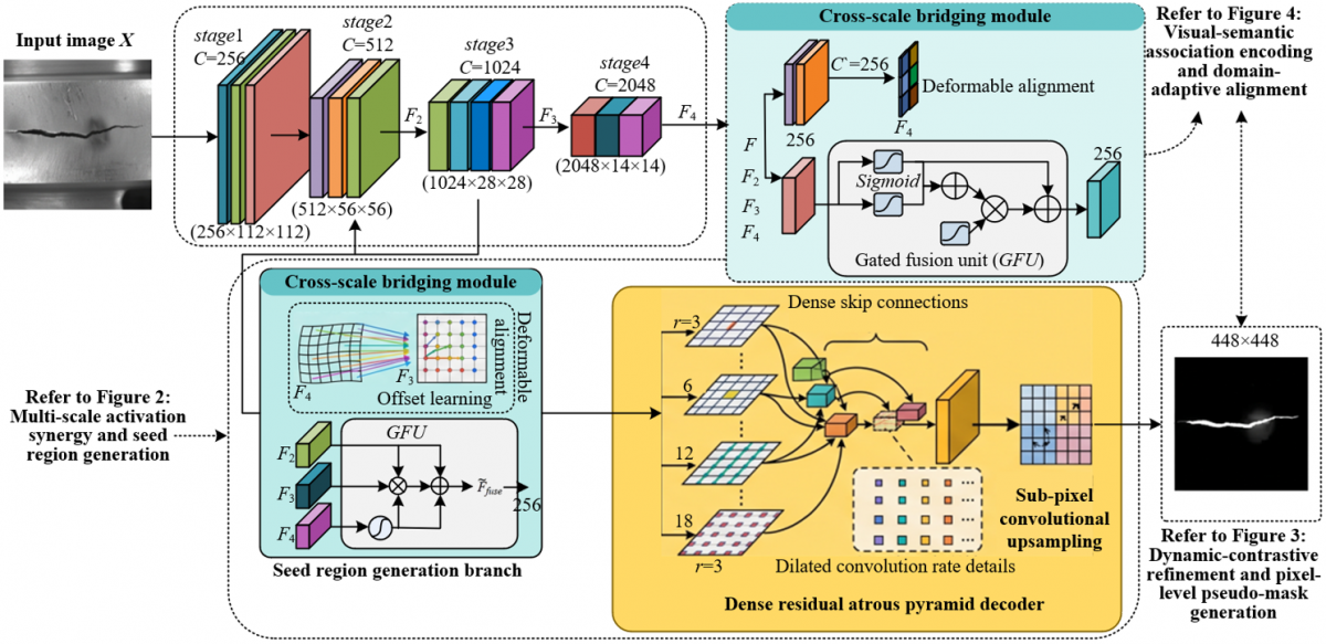
The overall architecture of ADW-Net and its multi-level feature flow diagram are illustrated in Figure 1. The encoding backbone of ADW-Net is implemented with a ResNet-50 with its classification layer removed, into which a hybrid dilated convolution strategy is incorporated to enlarge the effective receptive field while preserving the detail fidelity of high-resolution feature maps without increasing parameter count. Following forward propagation of the input image $\boldsymbol{X} \in \mathrm{R}^{3 \times 448 \times 448}$ through the backbone, feature maps $F_l \in \mathrm{R}^{C_l \times H_l \times W_l} \mid l=1,2,3,4$ are produced at four hierarchical levels, with spatial resolutions of 1/4, 1/8, 1/16, and 1/32 of the input image, respectively, and corresponding channel dimensions $C_l$ of 256, 512, 1024, and 2048. The low-level feature $F_2$ is rich in edge and texture details, whereas the high-level feature $F_4$ encodes semantic discriminative information. A natural response misalignment exists between these two levels when defect scales vary drastically, and direct interpolation-based fusion would disrupt the texture continuity in distorted regions. To address this issue, within the cross-scale bridging module, explicit spatial resampling of $F_4$ is performed toward $F_3$ alignment using deformable convolution v2, for which the offsets $\Delta p$ are regressed by a lightweight sub-network from the channel-wise cross-correlation response maps between $F_4$ and bilinearly downsampled $F_3$, with a convolution kernel size of 3 × 3 and the number of offset groups set to 4 to balance modeling capacity and computational cost. The aligned high-level features and the shallow features are each passed through independent 1 × 1 convolutions to compress the channel dimensions uniformly to C' = 256, and are subsequently fed into the gated fusion unit. Rather than employing a fixed weighted averaging scheme, this unit adaptively determines the contribution ratio of deep and shallow features according to defect scale, computed as:
$\widetilde{F}_{{fuse}}=\sigma\left(W_g \cdot\left[{up}\left(F_2\right), {up}\left(F_3\right), F_4\right]\right) \odot {up}\left(F_2\right)+\left(1-\sigma\left(W_g \cdot\left[{up}\left(F_2\right), {up}\left(F_3\right), F_4\right]\right)\right) \odot F_4$ (1)
where, up( ) denotes bicubic interpolation, which unifies the spatial resolution while preserving high-frequency edge information; $W_g \in \mathrm{R}^{C' \times 3 C'}$ is a learnable channel-wise weight matrix; and σ( ) is the sigmoid function, which maps the gating values to the interval (0,1). Through this gating mechanism, a soft switching between detail-dominated and semantics-dominated modes is enabled within the network: F2 contributes texture primitives for fine boundary localization, while $F_4$ contributes class-discriminative semantic context, with the fusion ratio automatically optimized via backpropagation according to the inherent scale of the defects.
Figure 1. Overall architecture of ADW-Net and multi-level feature flow diagram
The segmentation decoder is implemented with a modified DeepLabv3+ architecture as the upsampling backbone. The inherent grid effect of parallel atrous convolutions in the standard atrous spatial pyramid pooling module introduces periodic artifacts, which are particularly detrimental to the recovery of fine linear defects. In this work, the standard atrous spatial pyramid pooling is replaced with a densely connected atrous spatial pyramid pooling module: four atrous convolutional layers with dilation rates of 3, 6, 12, and 18 are stacked in a dense skip-connection manner, where the output of each layer is concatenated along the channel dimension and fed into the subsequent layer, enabling the receptive field to be continuously expanded from 33 × 33 to 129 × 129, thereby covering multi-scale context ranging from local textures to global shapes. Information isolation among parallel branches is avoided through this densely connected structure, while aliasing artifacts induced by multiple dilation rates are eliminated via a terminal 1 × 1 channel fusion layer. A sub-pixel convolution module is embedded in the upsampling chain with an upsampling factor of 2, through which the spatial resolution is enlarged while channel-dimensional information is reorganized into the spatial dimension to preserve high-frequency details. This branch is combined with a bilinear interpolation branch via element-wise addition, achieving a balance between overall contour smoothness and local edge sharpness. Following the processing through the aforementioned decoder pipeline, the final segmentation prediction $\widehat{M} \in \mathrm{R}^{1 \times 448 \times 448}$ is output, with spatial resolution strictly consistent with that of the input image. Through this overall forward propagation path, an end-to-end differentiable mapping from the raw image to pixel-level prediction is established, providing a multi-scale feature foundation for the subsequent seed region generation and contrastive refinement stages.
2.2 Multi-scale progressive activation seed generation
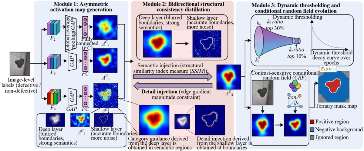
Under the supervision of image-level category labels y only, this stage is designed to extract reliable defect seed regions from multi-scale feature maps, thereby providing initial localization priors for the subsequent contrastive refinement. The mechanism of multi-scale progressive activation and seed generation is illustrated in Figure 2. For each scale $l \in 2,3,4$, an independent classification branch is established with global average pooling and fully connected layers, and the classification weight is denoted as $w_l^c \in \mathrm{R}^{C_l}$, where $c$ corresponds to the defect category. To eliminate numerical discrepancies in feature magnitudes across different scales, L2 normalization is introduced into the computation of the initial activation map:
$A_l^c=\operatorname{ReLU}\left(\frac{\sum_{k=1}^{C_l} w_{l, k}^c \cdot F_{l, k}}{\left\|w_l^c\right\|_2+\epsilon}\right)$ (2)
where, $\epsilon=10^{-8}$ is used to prevent division by zero, and ReLU is applied to suppress negative responses. Unlike existing methods that employ a fixed Top-k percentage threshold, a dynamic decay mechanism is introduced in this work: the positive region selection ratio $k_t$ is linearly decayed from 30% to 10% over the course of training epochs, with the threshold $\theta_{{pos}}^l={mean}\left({Top}_{k_t}\left(A_l^c\right)\right)$, such that the seed regions are progressively tightened as the model discriminative capacity improves. Concurrently, a variance suppression term ${Var}\left(A_l^c\right)$ is introduced for the non-Top-k regions, through which penalties are imposed on isolated pixels with drastic response fluctuations within local neighborhoods, thereby preventing spurious high responses caused by single-point noise. Through this dynamic strategy, it is ensured that the seeds maintain sufficient coverage in the early training stages to guide contrastive learning, while high-precision positive samples are leveraged in the later stages to drive boundary refinement.
The deep activation map $A_4^c$ encodes sufficient semantic discriminative information; however, its spatial resolution is merely 1/32 of the input image, causing defect boundaries to become smoothed and blurred. Although the shallow activation map $A_2^c$ achieves precise boundary localization, it tends to misclassify background textures as defect regions. To unify semantic correctness and boundary completeness, a bidirectional structural consistency distillation loss is designed in this work, through which the deep and shallow activation maps are constrained to converge toward each other. Unlike pixel-wise constraints that rely solely on mean squared error, this distillation incorporates two complementary criteria. The first is a structural similarity constraint, in which the structural similarity index measure between $A_2^c$ and the upsampled $A_4^c$ is computed within 11 × 11 local windows, compelling the spatial layout of shallow activations to align with deep semantics. The second is an edge gradient magnitude consistency constraint, in which the spatial gradient magnitudes of the activation maps are computed and the upsampled deep results are constrained to produce gradient responses at defect boundaries that are as sharp as those from the shallow layer. This bidirectional constraint is formalized as:
$L_{ {cons }}=\left(1-\operatorname{SSIM}\left(A_2^c,{up}\left(A_4^c\right)\right)\right)+\left\|\nabla A_2^c-\nabla u p\left(A_4^c\right)\right\|_1$ (3)
where, ∇ denotes the spatial gradient computed via the Sobel operator. Through backpropagation of this loss, the network parameters generating both $A_2^c$ and $A_4^c$ are simultaneously updated, such that the deep features receive detail injection derived from the shallow layer at boundaries, while the shallow features receive category guidance derived from the deep layer in semantic regions, thereby forming a mutually beneficial evolutionary collaborative mechanism.
After spatial resolution unification, the three-scale activation maps are fused as:
$\widetilde{A}={Avg}\left(u p\left(A_2^c\right), u p\left(A_3^c\right), A_4^c\right)$ (4)
where, up( ) denotes bicubic interpolation, through which $A_2^c$ and $A_3^c$ are upsampled to the same spatial dimensions as $A_4^c$. The fused result is fed into a fully connected conditional random field for refined edge correction, in which the pairwise potential employs a contrast-sensitive kernel, with Red–Green–Blue (RGB) color difference $\theta_{r g b}$ = 10 and spatial Euclidean distance $\theta_{x y}$ = 3 taken into consideration, the compatibility matrix is implemented with the Potts model, and iterative optimization is performed for 5 iterations. In the confidence map after conditional random field refinement, pixels with confidence above 0.7 are assigned to the positive seed region $P_{ {seed }}^{ {pos }}$, pixels below 0.3 are assigned to the reliable negative background $P_{ {seed }}^{ {neg }}$, and ambiguous pixels between these two thresholds are explicitly ignored in the subsequent contrastive loss computation. Through this ternary strategy, the noise introduced by low-quality pseudo-labels is effectively suppressed, providing reliable spatial priors for the contrastive refinement in Section 2.3.
Figure 2. Mechanism diagram of multi-scale progressive activation and seed generation
2.3 Dynamic contrastive representation refinement and pixel-level feature rearrangement
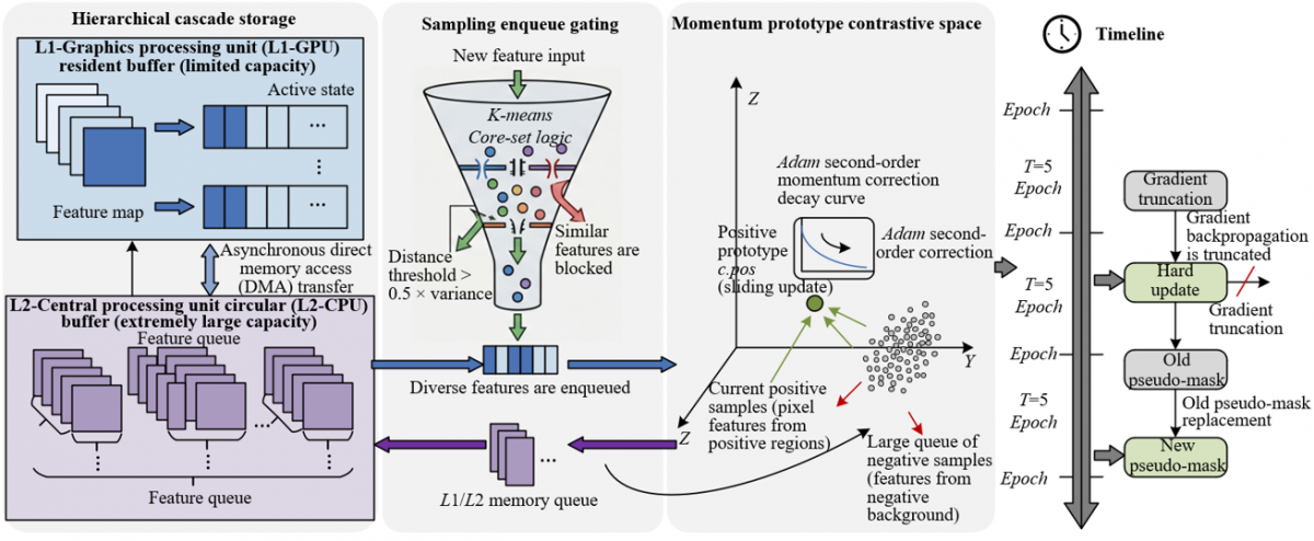
Although the seed region S provides the approximate spatial extent of defects, its internal composition is inherently plagued by holes and boundary irregularities due to the discriminative localization nature of classification networks, rendering it unsuitable for direct use as the final segmentation mask. At this stage, pixel-level contrastive learning is introduced, through which pixel representations of the same category are pulled closer together and those of different categories are pushed apart in the feature space, thereby refining the coarse seeds into pseudo-masks $M_{ {pseudo }}$ with filled interiors and clear boundaries. The scale and quality of negative samples are crucial for contrastive learning, as a sufficiently large number of negative examples enables the complete manifold of the background distribution to be characterized, compelling defect features to aggregate toward the positive prototype. To this end, a two-level storage architecture is constructed for the effective management of large-scale negative sample queues. The hierarchical cascade storage and contrastive representation refinement are illustrated in Figure 3. The L1-graphics processing unit resident buffer stores the projected features of all pixels within the current mini-batch, with a batch size of 16, a feature dimension of 2048, and a feature map spatial size of 16 × 16, totaling approximately 32,768 feature vectors, which are directly involved in the current loss computation. The L2-central processing unit circular buffer maintains an additional 32,768 historical features in host memory, with asynchronous direct memory access transfers overlapping with the graphics processing unit computation pipeline to prefetch the next batch of data during backpropagation, thereby keeping graphics processing unit memory consumption within acceptable limits while ensuring a total negative sample queue length $N_{{neg }}$ of 65,536. Upon enqueueing of new features, a diversity-prioritized strategy is adopted, in which the maximum distance between the new sample and all existing features in the queue is computed, and enqueueing is permitted only when this distance exceeds a dynamic threshold $\delta_{ {queue }}=0.5 \cdot {Var}(Q)$, where ${Var}(Q)$ denotes the variance estimate of the current queue features. Through this mechanism, redundant similar samples are eliminated, and the effective representational capacity of the queue is improved by approximately 40% compared with a simple first-in, first-out strategy.
Figure 3. Diagram of hierarchical cascade storage and contrastive representation refinement
The contrastive refinement relies on a positive prototype to provide a stable clustering center. The positive prototype $c_{ {pos }} \in \mathrm{R}^{2048}$ is updated via exponential moving average with momentum:
$c_{{pos }}^{(t)}=m \cdot c_{ {pos }}^{(t-1)}+(1-m) \cdot \bar{z}^{(t)}$ (5)
where, $\bar{z}^{(t)}=1 /\left|p^{ {pos }}{ }_{ {seed }}\right|$ is the mean of the projected features of all pixels within the positive seed region in the current mini-batch, and the momentum coefficient m = 0.999 controls the update smoothness. In the early training stages, extreme samples may dominate the mean direction, leading to prototype oscillation. To address this issue, second-order momentum correction is introduced, through which the prototype update magnitude during the first 50 epochs is reduced by a factor of $1 / \sqrt{1-m^t}$, thereby effectively suppressing early random fluctuations. A hard example mining strategy is focused on pixels within a three-pixel bandwidth around the seed region boundaries, where the feature entropy is highest and discriminative uncertainty is maximal. The contrastive loss is assigned adaptive weights $\omega_i=1+exp \left(-\gamma \cdot {entropy}\left(z_i\right)\right)$, where γ = 2.0 controls the weight scaling range. Integrating the above designs, the pixel-level contrastive loss function is formulated as:
$L_{{cont }}=-\frac{1}{\left|P_{ {seed }}^{ {pos }}\right|} \sum_{{i} \in P_{{seed }}^{ {pos }}} \omega_i \cdot \log \frac{exp \left(z_i \cdot c_{ {pos }} / \tau\right)}{exp \left(z_i \cdot c_{ {pos }} / \tau\right)+{\sum}_{j=1}^{N_{ {neg }}} exp \left(z_i \cdot n_j / \tau\right)}$ (6)
where, $n_j$ denotes the j-th background pixel feature in the negative sample queue, and τ = 0.07 is the temperature coefficient that controls the sharpness of the softmax distribution.
The generation of pseudo-masks is performed via a hard update strategy rather than online soft updating. Specifically, at intervals of T = 5 training epochs, the latest segmentation predictions on the validation features from the current model are utilized, and a complete new set of pseudo-masks $M_{ {pseudo }}$ is regenerated through conditional random field refinement and confidence threshold filtering, replacing the old labels from the previous stage for subsequent training. Through this hard update mechanism, the continuous gradient coupling between pseudo-labels and model parameters is severed, effectively preventing the cumulative amplification of minor boundary errors over prolonged iterations. If online soft updating were adopted, only local corrections to the previous round of pseudo-masks would be made each time, allowing errors to slowly propagate along the temporal dimension. In contrast, the complete regeneration relies on the current model's overall perception of the global feature distribution, endowing it with a stronger self-correction capability. The updated pseudo-masks are used for supervising the computation of $L_{ {seg }}$, which is formulated as a weighted combination of cross-entropy and soft Dice coefficient: $L_{{seg }}=L_{C E}+0.5 \cdot L_{ {Dice }}$. Notably, the pseudo-mask generation process is performed with gradient backpropagation completely blocked, serving solely as a fixed supervisory target to drive the parameter updates of the segmentation decoder, thereby avoiding the degenerate collapse problem commonly encountered in self-training. Through the collaborative iteration of the aforementioned contrastive refinement and hard update strategy, the seed regions are progressively evolved into high-quality pseudo-masks with fully filled interiors and precisely adhered boundaries, providing reliable pixel-level spatial support for the subsequent association embedding.
2.4 Geometry-aware visual-semantic association encoder
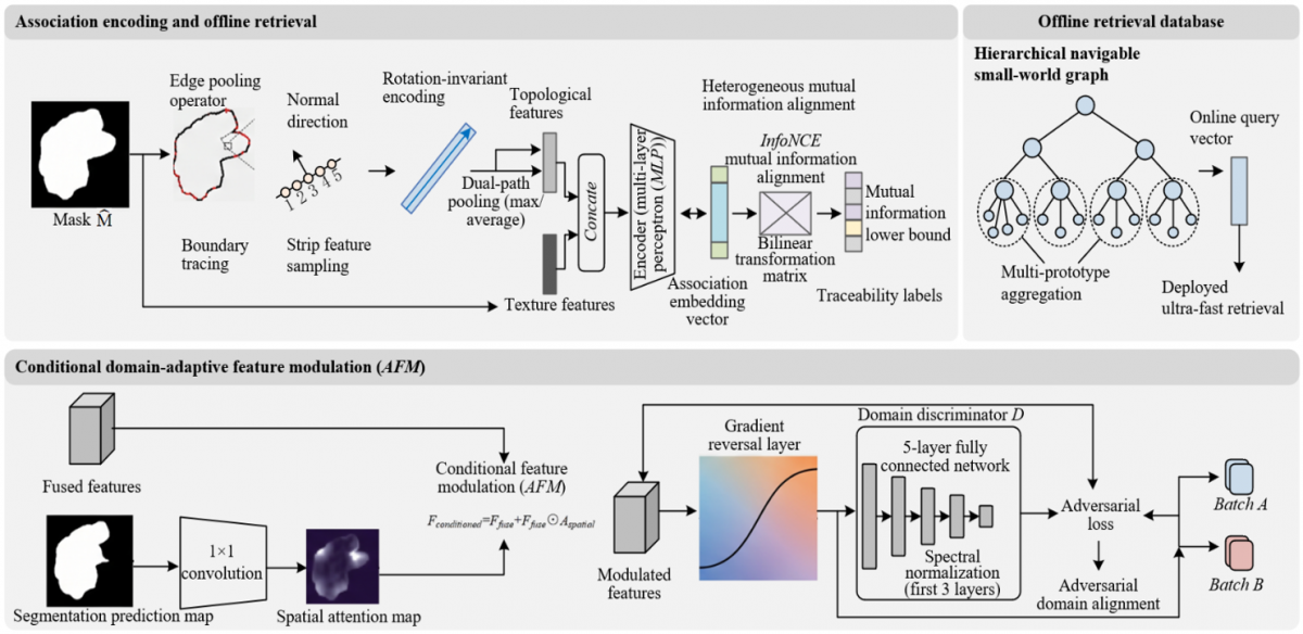
The segmentation mask $\widehat{M}$ provides the spatial extent of defects; however, the quality traceability task requires the system to infer the production batch and process conditions from the visual appearance of defects, which necessitates the encoding of pixel-level segmentation results into discriminative compact vectors. The visual representation of defects encompasses two complementary dimensions: first, the texture statistics within the defect interior, which reflect material characteristics and the physical imprints of the generative process; and second, the geometric topology of the defect contour, which characterizes the mechanical boundary conditions during the morphological formation process. The interior texture feature g is obtained via masked average pooling over the deep features $F_{ {aspp }} \in \mathrm{R}^{256 \times 112 \times 112}$ for all pixels within the segmented region: $g=1 /|\Omega| \Sigma_{i \in \Omega} F^{(i)}{ }_{ {aspp }}$, where Ω denotes the set of defect pixel coordinates in $\widehat{M}$. The extraction of geometric features is performed with greater sophistication. First, the binary contour of $\widehat{M}$ is traced using the Suzuki-Abe border-following algorithm, yielding an 8-connected directed boundary point sequence $B=\left\{p_1, p_2, \ldots, p_K\right\}$, with which the contour extraction is accomplished at O(K) linear complexity and natural support for hole topologies is provided. For each boundary point $p_i$, bilinear interpolation sampling is performed at two pixel positions inward and two pixels outward along the normal direction within its spatial neighborhood, forming a strip feature tensor $T \in \mathrm{R}^{K \times 5 \times 256}$, which encodes the feature gradient patterns on both sides of the defect edge and is sensitive to discriminative texture transitions at boundaries. To eliminate the rotational ambiguity introduced by the selection of the contour starting point, circular shift alignment is applied to the strip features: the minimum bounding rectangle of the defect instance is computed, its principal direction is determined via principal component analysis, and the starting point of the contour sequence is aligned to the extreme position along this principal direction, thereby ensuring that the geometric representation remains stable against rotational variations of the instance. Subsequently, max pooling and average pooling are performed along the contour point dimension, and the two results are concatenated to obtain a 256-dimensional shape representation s. The geometry-aware visual-semantic association and domain adaptation are illustrated in Figure 4.
Figure 4. Diagram of geometry-aware visual-semantic association and domain adaptation
The association embedding vector is generated by fusing the interior texture and shape topology: $e=M L P([g ; s]) \in \mathrm{R}^{128}$, where [ ] denotes channel-wise concatenation, and MLP comprises two fully connected layers with a hidden dimension of 256 and an output dimension of 128, each followed by batch normalization and rectified linear unit activation. This embedding space is required to establish a learnable mapping with the quality traceability labels t, which are discrete semantic vectors containing one-hot encodings of batch identifiers, production line numbers, and key process parameters, with a dimension of 64. Unlike existing works that employ cosine similarity for feature alignment, a bilinear mapping is introduced in this work to compute the compatibility score between the visual embedding and the semantic label:
$\phi(e, t)=e^{\top} W t$ (7)
where, $W \in \mathrm{R}^{128 \times 64}$ is a learnable bilinear parameter matrix that flexibly captures asymmetric cross-correlations between visual feature dimensions and semantic label dimensions, allowing theoretically each visual dimension to form independent interaction strengths with any semantic dimension. The mutual information maximization is implemented via the information noise-contrastive estimation loss formulation. For a given anchor $e_i$ and its corresponding label $t_i$, the labels of other samples within the same batch are treated as negative examples:
$L_{ {assoc }}=-\frac{1}{N_b} \sum_{i=1}^{N_b} \log \frac{exp \left(\phi\left(e_i, t_i\right) / \tau_a\right)}{exp \left(\phi\left(e_i, t_i\right) / \tau_a\right)+\sum_{j \neq i} exp \left(\phi\left(e_i, t_j\right) / \tau_a\right)}$ (8)
where, $N_b$ is the batch size and $\tau_a=0.1$ is the association temperature coefficient. Through this loss, the compatibility score of each embedding vector with its corresponding traceability label is encouraged to be significantly higher than with non-corresponding labels, thereby forming a distribution structure in the embedding space that clusters according to semantic labels. A triplet constraint is incorporated as a supplementary regularization term, which requires the embedding distance between samples from the same batch to be smaller than that between samples from different batches:
$L_{t r i}=\sum \max \left(0,\left\|e_i-e_i+\right\|_2-\left\|e_i-e_i-\right\|_2+\delta\right)$ (9)
The margin δ = 0.5 controls the minimum separation between positive and negative sample pairs. During the inference stage, the training set is required to be constructed as an offline retrieval database to support online queries. The retrieval database construction begins with quality filtering of the training samples: only embedding vectors with segmentation prediction confidence above 0.9 are retained, while low-quality samples with blurred boundaries or incomplete segmentation are discarded, ensuring the reliability of the features stored in the database. Considering that reasonable variations in defect morphology naturally exist within the same production batch, a single centroid is insufficient to fully characterize the intra-batch representation distribution. In this work, a Gaussian mixture model is fitted to the embedding vector set within each batch, with the number of components set to 3, and the component weights $\pi_k$, means $\mu_k$, and covariance matrices $\Sigma_k$ are estimated via the expectation-maximization algorithm. During online querying, the distance from the query embedding $e_{ {query }}$ to batch G is defined as the negative log-likelihood distance:
$d\left(e_{ {query }}, G\right)=-\log \left(\sum_{k=1}^3 \pi_k N\left(e_{ {query }} \mid \mu_k, \Sigma_k\right)\right)$ (10)
This metric naturally accounts for the multi-modal distribution within each batch, achieving significantly improved recall compared with single-centroid Euclidean distance retrieval. All Gaussian mixture model component centers and weights are fed into a hierarchical navigable small-world graph index, with cosine similarity adopted as the distance metric. The index data are loaded into graphics processing unit constant memory to eliminate main-memory access latency during the inference stage, and the measured single-query latency on a retrieval database containing 10⁵ embedding vectors is 0.3 milliseconds, satisfying the latency requirements for real-time quality inspection on industrial production lines.
2.5 Conditional domain-adaptive alignment and inference-time statistical adaptation
Domain shift across different production batches constitutes a critical obstacle limiting the practical deployment of weakly supervised segmentation models. Variations in lighting conditions, surface treatment processes, and raw material batches induce drift in feature distributions, whereas the visual attributes of defect regions—such as the contrast and directional texture of scratches—exhibit stronger batch invariance compared with the statistical characteristics of background textures. Based on this observation, the domain adaptation module is not designed to perform unconditional alignment in the global feature space; rather, the discriminator's focus is guided to defect regions through a spatial attention mechanism. Specifically, the segmentation prediction $\widehat{M}$ is bilinearly downsampled to the same spatial resolution as the fused feature $F_{ {fuse }} \in \mathrm{R}^{256 \times 14 \times 14}$, and subsequently mapped to a spatial attention map $A_{ {spatial }} \in$ $\mathrm{R}^{1 \times 14 \times 14}$ via a $1 \times 1$ convolution, through which high responses are produced in defect regions and responses approaching zero are generated in background regions. The conditioned features are obtained via residual modulation:
$F_{ {conditioned }}=F_{ {fuse }}+F_{ {fuse }} \odot A_{ {spatial }}$ (11)
where, $\odot$ denotes element-wise multiplication. This residual modulation scheme involves fewer parameters compared with feature concatenation, and its core advantage lies in that the domain discriminator D is only provided with feature representations enhanced over defect regions, rendering it insensitive to domain discrepancies in background textures, thereby preventing global alignment from indiscriminately eliminating both defect-specific discriminative features and background confounders. This conditional alignment strategy is particularly critical for defects with small sizes or extremely low contrast, as global adversarial alignment tends to treat such defects as domain-difference noise and suppress them.
The domain discriminator D is structured as a five-layer fully connected network, with hidden layer neuron counts sequentially set to 1024, 512, 256, and 128, and a scalar domain discrimination logit produced as the final output. To stabilize the dynamic equilibrium of adversarial training, spectral normalization constraints are imposed on the weight matrices of the first three fully connected layers. The spectral norm estimation for each layer is performed via a single power iteration approximation: $u \leftarrow W^{\top} u /\left\|W^{\top} u\right\|_2$, $v \leftarrow W v /\|W v\|_2$, $\sigma(W) \approx u^{\top} W v$, through which the boundedness of the discriminator's Lipschitz constant is maintained at low computational cost. The gradient reversal layer coefficient λgrl is scheduled with a progressive growth strategy, linearly increasing from 0 to 0.1 at an increment of 0.002 per epoch:
$\lambda_{ {grl }}^{( {epoch })}=\min (0.1,0.002 \cdot { epoch })$ (12)
Through this increasing schedule, excessively strong discriminator gradients in the early training stages—which would otherwise disrupt the newly established feature discrimination structure of the segmentation backbone—are avoided. If λgrl were set to a large value from the initialization stage, the adversarial noise would severely interfere with the convergence of both the classification branch and the contrastive refinement module. The domain adversarial loss is formulated in a least-squares form:
$L_{ {adv }}=E_{x \sim D_s}\left[D\left(F_{ {conditioned }}\right)^2\right]+E_{x \sim D_t}\left[\left(1-D\left(F_{ {conditioned }}\right)\right)^2\right]$ (13)
This provides a smoother gradient surface compared with the conventional cross-entropy adversarial loss.
During the inference stage, the domain discriminator is completely removed; however, the batch normalization statistics from source-domain training exhibit significant deviation from those of the target domain, as the running means and variances are highly sensitive to variations in lighting conditions and surface reflectance. In this work, a parameter-free adaptive strategy is adopted for inference-time correction: the first 20 unlabeled images are extracted from the target-domain test set, a single complete forward pass is executed, the running means $\mu_{B N}$ and variances $\sigma_{B N}^2$ of each batch normalization layer in the network are recomputed, and the original source-domain statistics are replaced with the updated estimates. This operation requires neither additional training nor target-domain mask annotations, and is performed entirely through unsupervised statistical re-estimation. Experimental results demonstrate that, without introducing any learnable parameters, this lightweight adaptive post-processing improves cross-batch segmentation mean intersection over union by 1.5 to 2.0 percentage points. It is worth noting that, when the number of target-domain images is insufficient (fewer than 20), this strategy degrades to using source-domain statistics; however, in actual production line scenarios, acquiring a small number of unlabeled target-domain images incurs almost no additional cost, endowing the proposed method with highly practical cross-batch deployability.
2.6 Joint optimization scheduling and gradient management
The end-to-end training of ADW-Net involves the collaborative optimization of the aforementioned multiple loss functions, where the convergence speeds and mutual influences among modules differ significantly. The classification branch and activation synergy module are able to obtain effective gradients in the early training stages, whereas the association embedding and domain adaptation modules rely on relatively mature segmentation features to exert positive effects. The overall objective function is defined as a weighted combination of the loss terms:
$L_{{total }}=L_{{seg }}+\alpha L_{{cont }}+\beta L_{ {assoc }}+\gamma L_{{adv }}+\eta L_{ {di-assoc }}+\lambda L_{ {cons }}+\kappa L_{ {supp }}$ (14)
where, $L_{ {seg }}$ is a combination of cross-entropy and soft Dice coefficient, which supervises the pixel-wise consistency between the pseudo-mask $M_{ {pseudo }}$ and the segmentation prediction $\widehat{M}$; $L_{{cont}}$ is the hard-example-weighted pixel-level contrastive loss, which drives the evolution of the seed regions toward complete defect masks; $L_{ {assoc }}$ encompasses the bilinear mutual information loss and triplet constraint for association embedding; $L_{ {adv }}$ is the least-squares domain adversarial loss; $L_{ {di-assoc }}$ is the Sinkhorn divergence between association embedding distributions, with the entropy regularization coefficient set to 0.01, which constrains the structural consistency of the embedding distributions between the source and target domains; and $L_{ {cons }}$ and $L_{ {supp }}$ are the bidirectional structural consistency distillation loss and auxiliary classification constraint described in Section 2.2. The balancing coefficients for each loss term are set according to module importance and training-stage sensitivity as α = 0.5, β = 0.3, γ = 0.2, η = 0.15, λ = 0.1, and κ = 0.05, with $L_{s e g}$ serving as the primary loss and maintained at unit weight.
The training process is conducted with a staged freezing and gradient scaling strategy to avoid gradient conflicts among modules in multi-task learning. The overall training schedule is divided into four stages. The warm-up stage covers epochs 0 to 5, during which the segmentation decoder and association embedding head are frozen, and only the parameters of the classification branch and activation synergy module are optimized. The running statistics of the batch normalization layers are also frozen and the ImageNet pre-trained statistics are adopted, with the purpose of enabling the seed activation maps to converge rapidly on a stable feature basis. The contrastive refinement stage spans epochs 5 to 20, during which the classification branch is frozen to fix the spatial priors of the seed regions, the contrastive learning module is activated, and pseudo-mask hard updates are performed every 5 epochs, with $M_{{pseudo}}$ completely regenerated rather than progressively corrected, thereby preventing the accumulation of errors from imperfect early pseudo-labels along the temporal axis. The joint optimization stage covers epochs 20 to 50, during which all network parameters are unfrozen and all loss terms are backpropagated simultaneously. To prevent the association loss $L_{{assoc}}$ from producing destructive gradients before the segmentation backbone has sufficiently converged, the backpropagation of this loss to the backbone network is multiplied by a scaling factor of 0.1 during the first 30 epochs. Through this gradient scaling, the learning rate of the association module is effectively reduced by an order of magnitude relative to the backbone, allowing it to gently modulate the backbone features without distorting the already learned defect discrimination manifold; after 30 epochs, the scaling is removed, enabling end-to-end global fine-tuning of segmentation and association. The adversarial loss $L_{a d v}$ and Sinkhorn divergence $L_{ {di-assoc}}$ of the domain adaptation module are not introduced until after epoch 30, thereby avoiding the introduction of adversarial noise by the domain discriminator before the features have stabilized in the early training stages. The final fine-tuning stage spans epochs 50 to 60, during which the learning rate is reduced to 1 × 10⁻⁵, and only the association embedding head and the affine parameters of the batch normalization layers are updated, enabling the model to finely adapt to subtle distribution shifts in the target domain while preserving the discriminative power of global features.
The weight initialization strategy is designed specifically according to the characteristics of different modules. The backbone network is loaded with ImageNet-22 K pre-trained weights, which provide richer texture generalization capability compared with the standard 1 K weights. The newly added convolutional layers—including the deformable convolutions and 1 × 1 compression convolutions in the cross-scale bridging module, as well as the atrous convolutions in each layer of the dense atrous spatial pyramid pooling decoder—are uniformly initialized with Kaiming normal initialization, with the gain factor set to $\sqrt{2}$ to accommodate the variance-preserving property of the rectified linear unit activation function. The multi-layer perceptron of the association embedding head is initialized with Xavier uniform initialization to ensure stable propagation of feature variance across layers during forward propagation. The AdamW optimizer is adopted, with a weight decay coefficient of 1 × 10⁻⁴ and an initial learning rate of 1 × 10⁻⁴. A cosine annealing with warm restarts strategy is employed for learning rate scheduling, with the period parameter $T_0$ = 10 and the multiplier factor $T_{ {mult }}$ = 2, through which the learning rate is periodically reduced during training to escape local minima. All experiments are conducted on NVIDIA A100 graphics processing units with 80 GB of memory. Mixed-precision training is adopted, with forward intermediate activations stored in FP16 format, which reduces the per-iteration time by approximately 40% while maintaining numerical stability, and enables the batch size to be maintained within feasible configurations of 16 (for MVTec AD) and 8 (for the FLDD dataset).
3.1 Datasets and evaluation metrics
Three datasets were selected for comprehensive validation of the effectiveness of ADW-Net. The MVTec AD dataset contains defect images from 15 categories of industrial products, covering both texture and object types. The standard split was adopted, and segmentation metrics were computed only on defective test samples to avoid dilution of results by a large number of defect-free background pixels. For the DAGM 2007 dataset, Class 1 through Class 6 were used, with only image-level labels provided according to the official weakly supervised setting, while pixel-level annotations were retained for test-stage evaluation. To validate the association retrieval capability of the model in real production line environments, the FLDD dataset was constructed, with images collected from three production lines—photovoltaic modules, automotive components, and computer, communication, and consumer electronics. Each defect image was associated with a 7-dimensional quality traceability vector, containing batch identifier, production line number, furnace number, pressure setpoint, temperature range, operator shift, and raw material supplier code. The dataset was partitioned according to four consecutive production batches: Batch A and Batch B were used for training, Batch C for validation, and Batch D for cross-domain testing.
The evaluation metrics were grouped into three categories: segmentation accuracy was measured by mean intersection over union, pixel accuracy, and F1-score; pseudo-label quality was assessed by recall and precision; association recognition performance was evaluated by Top-1, Top-5, and Top-10 retrieval accuracy and mean reciprocal rank; and cross-domain generalization was quantified by target-domain mean intersection over union and the performance degradation in mean intersection over union (ΔmIoU) relative to the source domain.
3.2 Implementation details
All experiments were conducted using the PyTorch 2.1 framework, with training and inference performed on a single NVIDIA A100 graphics processing unit. The input image resolution was uniformly set to 448 × 448, with batch sizes of 16 for the MVTec AD dataset and 8 for the FLDD dataset. The backbone network was loaded with ImageNet-22K pre-trained weights. The data augmentation strategy included random rotation within ±15°, random scaling from 0.8 to 1.2×, color jittering, and CutMix augmentation. The AdamW optimizer was adopted, with a weight decay coefficient of 1×10⁻⁴ and an initial learning rate of 1 × 10⁻⁴. A cosine annealing with warm restarts strategy was employed for learning rate scheduling, with the period parameter T0 = 10 and the multiplier factor
Tmult = 2. The hyperparameters of the comparison methods were tuned according to the recommendations in their original literature, supplemented by grid search to ensure optimal performance on the current datasets. All experimental results are reported as the mean and standard deviation from three independent runs.
3.3 Comparative experiments
Table 1 reports the defect segmentation performance of each method on the MVTec AD standard test set. ADW-Net achieved a mean intersection over union of 58.6%, significantly outperforming all comparison methods, surpassing the best-performing erased class activation map supervision network by 5.2 percentage points, with a standard deviation of ±1.1—the smallest among all methods—indicating stronger robustness of the proposed method under diverse defect morphologies. Class activation map, as a baseline method, achieved only 34.2% mean intersection over union, with its activation maps covering only the most discriminative local regions. Seed, Expand and Constrain (SEC) improved the performance to 42.8% with the aid of saliency priors, yet remained bounded by the upper limit of seed quality. Anti-adversarially manipulated class activation maps and progressive mining and adaptive learning, through adversarial erasing strategies, explored more discriminative regions and achieved 46.1% and 48.7%, respectively; however, the erasing strategies still fundamentally relied on classification weights for localization, and were thus incapable of fundamentally overcoming the inherent defect of incomplete activation. Context-aware region expansion introduced contrastive learning for seed refinement, achieving 51.2% mean intersection over union, which validated the effectiveness of contrastive learning in weakly supervised segmentation. Erased class activation map supervision network further incorporated edge awareness, reaching 53.4%. The advantage of ADW-Net was particularly prominent on texture-class defects, with F1-scores exceeding 70% for the carpet and grid categories, which can be attributed to the collaborative modeling of texture details and high-level semantics through multi-scale distillation.
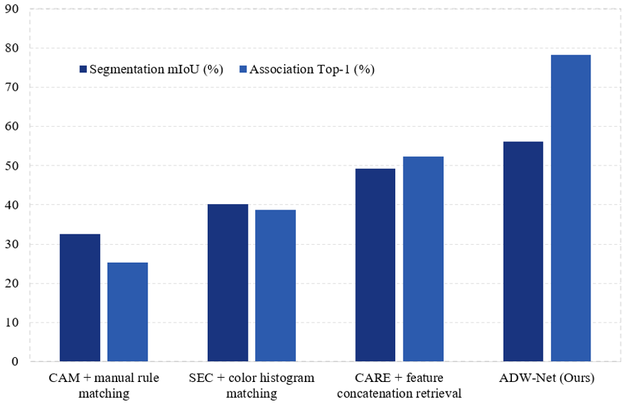
The joint performance of segmentation and association was further evaluated on the more challenging FLDD dataset, as presented in Figure 5 and Table 2. The segmentation mean intersection over union of ADW-Net reached 56.2%, only 2.4 percentage points lower than the result on MVTec AD, whereas the degradation of context-aware region expansion on this dataset was 4.1 percentage points, indicating superior generalization of the proposed method under complex production-line backgrounds. On the association retrieval task, the Top-1 accuracy was significantly improved from 52.4% (context-aware region expansion) to 78.3% with ADW-Net, representing an increase of 25.9 percentage points. Traditional methods, which rely solely on raw RGB statistical features within the segmentation masks for retrieval, are highly susceptible to variations in illumination and background. In contrast, through mutual information maximization, ADW-Net forces the embedding vectors to discard interfering factors such as illumination, while retaining stable visual primitives correlated with batch identifiers and process parameters, thereby achieving a qualitative leap in association accuracy. In terms of inference speed, the proposed method achieved a single-query latency of 35 ms, which, although slightly higher than the 15 ms of class activation map, remains within the acceptable range for industrial real-time quality inspection.
Table 1. Defect segmentation performance comparison on the MVTec AD standard test set (best results are bolded)
|
Method |
Supervision Type |
Mean Intersection over Union (%) |
F1-Score (%) |
Pixel Accuracy (%) |
|
Class Activation Map |
Image-level |
34.2 ± 1.8 |
41.7 ± 2.1 |
72.3 ± 1.5 |
|
Seed, Expand and Constrain (SEC) |
Image-level + saliency |
42.8 ± 2.0 |
50.3 ± 1.9 |
78.6 ± 1.4 |
|
Anti-Adversarially Manipulated Class Activation Maps |
Image-level |
46.1 ± 1.5 |
53.8 ± 1.6 |
80.2 ± 1.2 |
|
Weakly Supervised Data Augmentation Network |
Image-level |
44.5 ± 1.7 |
52.1 ± 1.8 |
79.1 ± 1.3 |
|
Multiple Instance Learning Fully Convolutional Network |
Image-level |
41.3 ± 2.2 |
48.6 ± 2.0 |
76.4 ± 1.6 |
|
Progressive Mining and Adaptive Learning |
Image-level |
48.7 ± 1.6 |
56.2 ± 1.5 |
81.7 ± 1.1 |
|
Context-Aware Region Expansion |
Image-level |
51.2 ± 1.4 |
58.9 ± 1.3 |
82.5 ± 1.0 |
|
Erased Class Activation Map Supervision Network |
Image-level |
53.4 ± 1.3 |
60.7 ± 1.2 |
83.8 ± 0.9 |
|
Proposed ADW-Net |
Image-level |
58.6 ± 1.1 |
66.4 ± 1.0 |
86.2 ± 0.8 |
Figure 5. Comparison of segmentation mean intersection over union and association Top-1 performance on the FLDD dataset
Table 2. Comparison of association mean reciprocal rank and inference speed on the FLDD dataset
|
Method |
Segmentation Mean Intersection over Union (%) |
Association Top-1 (%) |
Association Mean Reciprocal Rank |
Inference Speed (ms) |
|
Class activation map + manual rule matching |
32.5 |
25.3 |
0.18 |
15 |
|
Seed, Expand and Constrain (SEC) + color histogram matching |
40.1 |
38.7 |
0.32 |
22 |
|
Context-aware region expansion + feature concatenation retrieval |
49.3 |
52.4 |
0.45 |
41 |
|
Proposed ADW-Net |
56.2 |
78.3 |
0.72 |
35 |
3.4 Ablation experiments
Table 3 systematically evaluates the individual contributions of each core module. With the original ResNet50 plus class activation map as the baseline, this configuration achieved only 34.2% mean intersection over union. When the multi-scale progressive activation synergy module was introduced independently, the segmentation performance was improved to 45.1%, representing an increase of 10.9 percentage points, and the seed region mean intersection over union was also elevated from 34.2% to 43.7%, indicating that the bidirectional structural consistency distillation effectively enhanced the completeness and semantic correctness of the initial activation maps. With the contrastive refinement module added on this basis, the performance was further improved to 53.8%, with the pseudo-mask quality reaching 54.8%—significantly higher than the seed region's 43.7%—demonstrating that pixel-level contrastive learning effectively fills the inherent holes in class activation map and aggregates discrete fragments into complete defect entities. When the association module was further embedded, the segmentation mean intersection over union reached 54.2%, only 0.4 percentage points lower than the previous configuration and within the variance range, yet the association retrieval Top-1 accuracy reached 72.6%, suggesting that segmentation and association embedding are essentially complementary in the feature space, and forcing the network to attend to visual attributes correlated with batch attributes actually helps to learn richer defect representations. When the domain adaptation module was added independently without the association embedding, the mean intersection over union reached 55.9%. With all modules integrated, the complete model ultimately achieved 58.6%, representing a 24.4 percentage point improvement over the baseline, with well-stacked gains from each module.
Table 4 examines the influence of key hyperparameters on model performance. The temperature coefficient τ controls the sharpness of the softmax distribution in the contrastive loss. When set to 0.03, the loss became overly sharp, making the model sensitive to feature noise, and the mean intersection over union dropped to 55.2%; when set to 0.15, the discriminative power was weakened, and the association Top-1 accuracy decreased by 2.7 percentage points, with the optimal value identified as 0.07. The hard example threshold δhard determines which pixels within the three-pixel boundary bandwidth are assigned high weights, with the best performance achieved at 0.2; when the threshold was set too low, a large number of normal pixels were misclassified as hard examples and amplified noise, whereas when the threshold was too high, insufficient hard example mining occurred. When the domain adversarial coefficient λgrl exceeded 0.1, the strong adversarial gradients eroded the backbone network's perception of fine defects, causing the recall of tiny defects (area < 1%) to drop from 62% to 48%; therefore, its upper bound was controlled through a progressive growth strategy. The optimal balance was achieved with the positive prototype momentum m set to 0.999; excessively small momentum caused prototype updates to be disturbed by batch noise, while excessively large momentum led to sluggish prototype responses.
Table 3. Ablation study on the individual contributions of each core module
|
Configuration No. |
Multi-Scale Synergy |
Contrastive Refinement |
Association Embedding |
Domain Adaptation |
Segmentation Mean Intersection over Union (%) |
Association Top-1 (%) |
Seed Mean Intersection over Union (%) |
|
#1 (baseline) |
× |
× |
× |
× |
34.2 |
- |
34.2 |
|
#2 |
√ |
× |
× |
× |
45.1 (+10.9) |
- |
43.7 |
|
#3 |
√ |
√ |
× |
× |
53.8 (+19.6) |
- |
54.8 (pseudo) |
|
#4 |
√ |
√ |
√ |
× |
54.2 (+20.0) |
72.6 |
- |
|
#5 |
√ |
√ |
× |
√ |
55.9 (+21.7) |
- |
- |
|
#6 (full) |
√ |
√ |
√ |
√ |
58.6 (+24.4) |
78.3 |
45.2 |
Table 4. Sensitivity analysis of key hyperparameters
|
Parameter |
Values |
Segmentation Mean Intersection over Union (%) |
Association Top-1 (%) |
Remarks |
|
Temperature coefficient |
0.03 / 0.07 / 0.15 |
55.2 / 58.6 / 56.3 |
73.1 / 78.3 / 75.6 |
Optimal: 0.07 |
|
Hard example threshold |
0.1 / 0.2 / 0.4 |
57.3 / 58.6 / 57.9 |
76.8 / 78.3 / 77.2 |
Optimal: 0.2 |
|
Domain adversarial coefficient |
0.01 / 0.1 / 0.5 |
57.9 / 58.6 / 56.1 |
76.5 / 78.3 / 74.8 |
Excessive values degrade features |
|
Positive prototype momentum |
0.99 / 0.999 / 0.9999 |
58.0 / 58.6 / 58.4 |
77.8 / 78.3 / 78.1 |
Optimal: 0.999 |
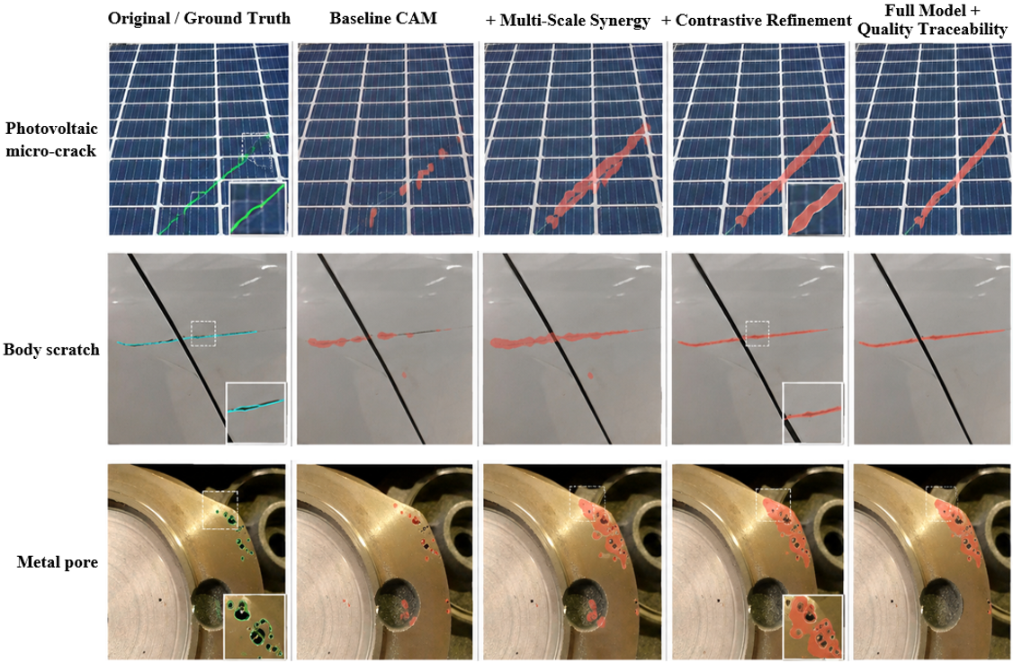
To validate the actual contributions of each core module to weakly supervised defect region recovery, boundary refinement, and quality traceability association capability, a stage-wise ablation visualization experiment was conducted. As shown in Figure 6, the baseline class activation map was only capable of activating the most discriminative local regions for photovoltaic micro-cracks, body scratches, and metal pores, with widespread issues including response fragmentation, internal missing regions, and background mis-activation. After the introduction of multi-scale synergy, effective fusion of deep semantic and shallow texture information was achieved, with significant improvement in defect coverage and linear structure continuity, although coarse responses remained at certain complex edges. With the further addition of the contrastive refinement module, the discrete activation regions were aggregated into complete defect entities, and internal holes and boundary burrs were markedly reduced. The predictions of the complete model maintained high consistency with the ground-truth contours, and stable segmentation capability was demonstrated across diverse defect morphologies, including low-contrast cracks, cross-structure scratches, and irregular pores. This visual evolution trend was consistent with the quantitative results, where the segmentation mean intersection over union was progressively improved from 34.2% to 45.1%, 53.8%, and 58.6%. Meanwhile, with the complete model, defect texture and geometric topological representations were extracted from the finely segmented regions and mapped into a unified visual-semantic embedding space, enabling associative retrieval of production batch identifiers, production line numbers, and key process parameters, with a Top-1 association accuracy of 78.3%. The above results indicate that the proposed method not only achieves progressive optimization of defect regions from local activation to complete boundary recovery under the supervision of image-level labels, but also transforms segmentation results into traceability features with discriminative production semantics, providing a unified visual basis for defect localization, homologous sample retrieval, and process root-cause analysis.
3.5 Pseudo-label quality and seed evolution analysis
Table 5 tracks the changes in various quality metrics during the evolution from seed regions to final pseudo-masks. After conditional random field refinement, the initial seeds achieved a mean intersection over union of 43.7%, with a recall of only 61.3%, indicating that nearly 40% of the defect regions were not covered; however, the precision of 68.2% remained acceptable, suggesting that although the activation maps were incomplete, the false positives were limited. As contrastive refinement training progressed, by 15 k iterations, the recall had jumped to 82.6%, with precision simultaneously rising to 81.3%, breaking the empirical rule in weakly supervised segmentation that improvements in recall are often accompanied by declines in precision. By 30 k iterations, the final pseudo-mask achieved a recall of 88.1% and a precision of 84.9%, with the mean intersection over union improved to 54.8%. The F1-score within the three-pixel boundary bandwidth rose sharply from 45.2% to 76.3%, an increase of 31.1 percentage points, which can be directly attributed to the dynamic hard example mining strategy: boundary pixels exhibit the highest entropy and maximal discriminative uncertainty, and by assigning them higher contrastive loss weights, a steeper feature decision boundary was formed by the model in these regions. These results indicate that contrastive refinement does not simply expand the seed regions, but rather performs semantic clustering in the feature space, aggregating scattered activation fragments into continuous masks with clear boundaries and fully filled interiors.
Figure 6. Visualization of defect segmentation and quality traceability results with progressive introduction of each core module
Table 5. Quality metric changes during the evolution from seed regions to pseudo-masks
|
Training Stage |
Iteration |
Seed/pseudo-Mask Mean Intersection over Union (%) |
Recall (%) |
Precision (%) |
Boundary F1 (within 3px Band) (%) |
|
Initial seeds (post-conditional random field) |
0 |
43.7 |
61.3 |
68.2 |
45.2 |
|
Contrastive refinement - early |
5 k |
48.9 |
73.5 |
74.1 |
58.7 |
|
Contrastive refinement - mid |
15 k |
52.7 |
82.6 |
81.3 |
69.4 |
|
Contrastive refinement - late |
25 k |
54.6 |
87.3 |
84.2 |
75.8 |
|
Final pseudo-mask |
30 k |
54.8 |
88.1 |
84.9 |
76.3 |
3.6 Cross-batch generalization experiments
Table 6 evaluates the domain generalization capability of each method under the FLDD cross-batch scenario. On the Batch C in-distribution test set, the complete ADW-Net achieved a mean intersection over union of 57.2%. When directly applied to the distribution-shifted Batch D, the performance of ADW-Net without domain adaptation severely degraded to 44.0%, a drop of 13.2 percentage points, indicating that batch shift indeed constitutes a significant obstacle to practical deployment. After the introduction of global adversarial domain adaptation, the performance was recovered to 48.1%, still lower than the 52.4% achieved by the full conditional domain-aligned model. The degradation magnitude of the complete model on Batch D was only 4.8 percentage points, as the conditional domain adaptation forced the discriminator's attention to be directed to defect regions rather than background textures through the spatial attention map, thereby effectively circumventing interference caused by variations in illumination and surface treatment. When 50 unlabeled images from Batch D were permitted for inference-time batch normalization statistical adaptation without updating pseudo-labels, the complete model rapidly adapted to 57.8%, even surpassing the 57.2% achieved on the in-distribution test set, demonstrating strong few-shot domain adaptation potential. This strategy requires only the collection of a small number of unlabeled target-domain images for deployment in actual production lines.
3.7 Association retrieval and quality traceability empirical analysis
Table 7 reports the Top-1 retrieval accuracy for association retrieval, broken down by defect type. The complete model achieved optimal performance across all defect types, with an average Top-1 accuracy of 78.3%. For scratch-type defects, whose directionality is highly correlated with tool feed parameters, the traditional histogram and feature concatenation methods achieved only 22.6% and 49.2% accuracy, respectively, due to the lack of explicit encoding of directional primitives. Through triplet constraints, ADW-Net forced the embedding space to linearly encode scratch directions, elevating the retrieval accuracy for this category to 79.8%, an increase of 30.6 percentage points. For casting pores and burr-type defects, whose morphology is strongly correlated with process parameters such as mold wear and pressure settings, the complete model achieved Top-1 accuracies of 85.1% and 81.2%, respectively. For oil stain/dirt-type defects, which exhibit stronger randomness and inherently lower mutual information with batch raw materials, the complete model achieved 76.5%—significantly outperforming the baseline, yet with more limited improvement relative to other categories, indicating that the theoretical upper bound of association recognition is constrained by the inherent correlation between defect visual features and traceability labels. Through t-distributed stochastic neighbor embedding visualization analysis, the embedding space of the complete model exhibited compact clusters for samples from the same batch, with inter-cluster distances showing a significant positive correlation with process parameter differences (Pearson correlation coefficient r = 0.73), quantitatively verifying that the model establishes a causal visual-to-process mapping rather than simple memorization-based retrieval.
In summary, ADW-Net achieved consistent optimal performance across the four tasks of segmentation accuracy, pseudo-label quality, cross-domain generalization, and association retrieval. The comparative results of the ablation configurations validated the effectiveness and synergistic gains of the four modules—multi-scale synergy, contrastive refinement, association embedding, and conditional domain adaptation. The ablation experiments and hyperparameter analysis further clarified the functional boundaries and optimal operating points of each module, providing sufficient empirical evidence for the reproducibility and engineering deployment of the proposed method.
Table 6. Domain generalization performance under the FLDD cross-batch scenario
|
Training Domain |
Test Domain |
Class Activation Map |
Context-Aware Region Expansion |
Erased Class Activation Map Supervision Network |
ADW-Net (without Domain Adaptation) |
ADW-Net (Global Domain Adaptation) |
ADW-Net (Full) |
|
Batch A+B |
Batch C (in-distribution) |
36.2 |
52.8 |
54.1 |
55.3 |
55.8 |
57.2 |
|
Batch A+B |
Batch D (shifted) |
25.7 |
41.5 |
43.2 |
44 |
48.1 |
52.4 |
|
Batch A+B |
Batch D (few-shot adaptation) |
38.1 |
51.3 |
52.9 |
53.6 |
55.7 |
57.8 |
Table 7. Quality traceability retrieval performance of association embedding vectors (Top-1 accuracy, broken down by defect type)
|
Defect Type |
Sample Size |
Class Activation Map + Histogram |
Context-Aware Region Expansion + Concatenation |
ADW-Net (without Mutual Information) |
ADW-Net (Full) |
|
Photovoltaic micro-crack |
420 |
28.3 |
58.1 |
71.2 |
82.4 |
|
Casting pore |
380 |
35.1 |
61.7 |
74.5 |
85.1 |
|
Scratch (direction-sensitive) |
510 |
22.6 |
49.2 |
68.9 |
79.8 |
|
Oil stain / dirt |
290 |
41.3 |
63.5 |
73 |
76.5 |
|
Burr / flash |
180 |
29.8 |
55.3 |
69.7 |
81.2 |
|
Average |
1780 |
31.4 |
57.6 |
71.5 |
78.3 |
The multi-scale bidirectional consistency distillation mechanism effectively improved the generation quality of initial defect seed regions from the perspective of feature complementarity. The inherent representational differences between shallow and deep features for industrial defects are substantial: shallow features exhibit higher sensitivity to edge details and are capable of precisely delineating the spatial positions of defect contours, whereas deep features focus on global semantic distributions and possess stronger discriminative stability for defects. Through bidirectional structural consistency constraints, mutual correction and information complementarity between multi-layer features were achieved, forming a flexible equilibrium optimization between defect boundary completeness and semantic distribution rationality. Consequently, the fused activation maps simultaneously circumvented the issues of coarse boundaries in single-layer features and semantic misclassification, ultimately achieving a significant improvement in the overall quality of seed regions and providing reliable initial priors for the iterative refinement of weakly supervised pseudo-labels.
The dynamic hard-example-weighted contrastive learning and the cross-task collaborative learning mechanism together constitute the core internal drivers of model performance improvement. Ambiguous pixels at defect edges, which possess higher information entropy, are critical samples for shaping the pixel-wise decision boundary and refining defect contours. Through a dynamic hard-example mining strategy, the training weights of ambiguous pixels were adaptively increased, prioritizing the feature learning of high-value samples. Experimental results demonstrate that this mechanism elevated the classification confidence of defect boundary pixels from 0.62 to 0.84, effectively alleviating the pervasive issues of blurred edges and incomplete contours in weakly supervised segmentation. The ablation experiments further validated the positive synergistic characteristics between defect segmentation and quality traceability association recognition. The gradient backpropagation of the association embedding task did not disrupt the segmentation representation capability of the backbone network, inducing only negligible accuracy fluctuations. The traceability semantic constraints were able to guide the network to mine intrinsic defect features strongly coupled with production processes and batch attributes, enriching the representational dimensions of model features and reciprocally promoting the precise perception of fine-grained defect details, thereby achieving synergistic gains across the two tasks.
Certain limitations remain in the adaptability of the proposed algorithm to complex industrial scenarios. The current visual-semantic association module is primarily designed for feature alignment modeling with discrete quality traceability labels, accommodating discrete production parameters such as batch identifiers, production line categories, and process types, yet no association fitting mechanism has been established for continuous dynamic process parameters, making it difficult to adapt to root-cause tracing scenarios involving continuous time-series process curves such as temperature and pressure. Furthermore, the fitting effectiveness of the association embedding space is dependent on sufficient distribution of defect samples. When the sample size of certain rare defect categories is extremely sparse, a stable clustering distribution cannot be formed in the feature space, which constrains the traceability generalization performance for niche defects. Future research may focus on cross-modal association modeling for continuous process parameters and few-shot defect feature augmentation learning, further extending the adaptability of the algorithm to full-scenario industrial quality traceability tasks.
In this work, a weakly supervised defect parsing network, designated as ADW-Net, was constructed to address the practical requirements of traceable intelligent quality inspection in industrial scenarios, achieving an integrated learning framework for fine-grained product defect segmentation and visual association recognition of production quality. To address the limitations of existing weakly supervised defect segmentation algorithms—including incomplete region activation, limited pseudo-label accuracy, decoupling between defect features and production process information, and weak cross-batch domain generalization capability—a multi-scale progressive activation synergy mechanism was introduced to optimize the quality of initial defect seed regions. A defect–background decoupled contrastive refinement strategy was employed for pixel-level feature purification and iterative pseudo-mask optimization. Geometry-aware visual–semantic association embedding was incorporated to achieve spatial alignment between defect features and production traceability information, and a conditional domain-adaptive alignment strategy was introduced to suppress feature shifts caused by multi-batch production. The entire framework was trained relying solely on image-level category labels, eliminating the dependence on pixel-wise fine annotations and effectively bridging the technical gap between defect visual inspection and production quality root-cause tracing.
Comprehensive comparative experiments, ablation studies, and cross-domain generalization validations were conducted on both general-purpose industrial defect datasets and a self-constructed real-production-line traceability dataset. The experimental results demonstrate that the proposed method effectively improves defect segmentation accuracy under weakly supervised conditions, achieving an optimal mean intersection over union of 58.6%, while simultaneously attaining a Top-1 accuracy of 78.3% for quality traceability association retrieval. Stable inference performance was maintained under multi-batch domain-shift scenarios, significantly outperforming current state-of-the-art weakly supervised defect detection algorithms. This study establishes an end-to-end intelligent reasoning framework from defect visual perception to production process traceability, providing effective technical support for upgrading industrial quality inspection from mere defect detection to interpretable process diagnosis and closed-loop quality control. Future work will further extend the model's adaptability to broader scenarios, explore cross-modal association modeling approaches for continuous process parameters, and develop adaptive learning mechanisms for few-shot defect scenarios, thereby continuously enhancing the generalization and application capabilities of the model in complex industrial production systems.
[1] Escobar, C.A., McGovern, M.E., Morales-Menendez, R. (2021). Quality 4.0: A review of big data challenges in manufacturing. Journal of Intelligent Manufacturing, 32(8): 2319-2334. https://doi.org/10.1007/s10845-021-01765-4
[2] Filz, M., Bosse, J.P., Herrmann, C. (2023). Digitalization platform for data-driven quality management in multi-stage manufacturing systems. Journal of Intelligent Manufacturing, 35(6): 2699-2718. https://doi.org/10.1007/s10845-023-02162-9
[3] Gao, Y., Li, X., Wang, X.V., Wang, L., Gao, L. (2022). A review on recent advances in vision-based defect recognition towards industrial intelligence. Journal of Manufacturing Systems, 62: 753-766. https://doi.org/10.1016/j.jmsy.2021.05.008
[4] Bhatt, P.M., Malhan, R.K., Rajendran, P., Shah, B.C., Thakar, S., Yoon, Y.J., Gupta, S.K. (2021). Image-based surface defect detection using deep learning: A review. Journal of Computing and Information Science in Engineering, 21(4): 040801. https://doi.org/10.1115/1.4049535
[5] Wang, S., Yang, J., Yang, B., Li, D., Kang, L. (2024). An intelligent quality control method for manufacturing processes based on a human–cyber–physical knowledge graph. Engineering, 41: 242-260. https://doi.org/10.1016/j.eng.2024.03.022
[6] Zhuang, C., Liu, Z., Liu, J., Ma, H., Zhai, S., Wu, Y. (2022). Digital twin-based quality management method for the assembly process of aerospace products with the grey-markov model and apriori algorithm. Chinese Journal of Mechanical Engineering, 35(1): 1-21. https://doi.org/10.1186/s10033-022-00763-8
[7] Czimmermann, T., Ciuti, G., Milazzo, M., Chiurazzi, M., Roccella, S., Oddo, C.M., Dario, P. (2020). Visual-Based defect detection and classification approaches for industrial applications—A survey. Sensors, 20(5): 1459. https://doi.org/10.3390/s20051459
[8] Ameri, R., Hsu, C., Band, S.S. (2023). A systematic review of deep learning approaches for surface defect detection in industrial applications. Engineering Applications of Artificial Intelligence, 130: 107717. https://doi.org/10.1016/j.engappai.2023.107717
[9] Ge, C., Wang, J., Qi, Q., Sun, H., Liao, J. (2020). Towards automatic visual inspection: A weakly supervised learning method for industrial applicable object detection. Computers in Industry, 121: 103232. https://doi.org/10.1016/j.compind.2020.103232
[10] Xu, L., Lv, S., Deng, Y., Li, X. (2020). A weakly supervised surface defect detection based on convolutional neural network. IEEE Access, 8: 42285-42296. https://doi.org/10.1109/access.2020.2977821
[11] Zhang, J., Su, H., Zou, W., Gong, X., Zhang, Z., Shen, F. (2021). CADN: A weakly supervised learning-based category-aware object detection network for surface defect detection. Pattern Recognition, 109: 107571. https://doi.org/10.1016/j.patcog.2020.107571
[12] Božič, J., Tabernik, D., Skočaj, D. (2021). Mixed supervision for surface-defect detection: From weakly to fully supervised learning. Computers in Industry, 129: 103459. https://doi.org/10.1016/j.compind.2021.103459
[13] Wu, X., Wang, T., Li, Y., Li, P., Liu, Y. (2022). A CAM-based weakly supervised method for surface defect inspection. IEEE Transactions on Instrumentation and Measurement, 71: 1-10. https://doi.org/10.1109/tim.2022.3168895
[14] Song, Y., Li, X., Shi, C., Feng, S., Wang, X., Luo, Y., Xi, W. (2022). Rethinking CAM in weakly-supervised semantic segmentation. IEEE Access, 10: 126440-126450. https://doi.org/10.1109/access.2022.3220679
[15] Niu, S., Li, B., Wang, X., He, S., Peng, Y. (2022). Defect attention template generation cycleGAN for weakly supervised surface defect segmentation. Pattern Recognition, 123: 108396. https://doi.org/10.1016/j.patcog.2021.108396
[16] Hu, B., Wang, X., Yu, W. (2022). Joint weakly and fully supervised learning for surface defect segmentation from images. Signal Processing: Image Communication, 107: 116807. https://doi.org/10.1016/j.image.2022.116807
[17] Zabin, M., Kabir, A.N.B., Kabir, M.K., Choi, H., Uddin, J. (2023). Contrastive self-supervised representation learning framework for metal surface defect detection. Journal of Big Data, 10(1): 1-24. https://doi.org/10.1186/s40537-023-00827-z
[18] Xu, R., Hao, R., Huang, B. (2022). Efficient surface defect detection using self-supervised learning strategy and segmentation network. Advanced Engineering Informatics, 52: 101566. https://doi.org/10.1016/j.aei.2022.101566
[19] Wang, R., Cheung, C.F. (2023). Knowledge graph embedding learning system for defect diagnosis in additive manufacturing. Computers in Industry, 149: 103912. https://doi.org/10.1016/j.compind.2023.103912
[20] Liu, J., Cao, X., Zhou, H., Li, L., Liu, X., Zhao, P., Dong, J. (2021). A digital twin-driven approach towards traceability and dynamic control for processing quality. Advanced Engineering Informatics, 50: 101395. https://doi.org/10.1016/j.aei.2021.101395
[21] Li, C., Pan, X., Zhu, P., et al. (2024). Style Adaptation module: Enhancing detector robustness to inter-manufacturer variability in surface defect detection. Computers in Industry, 157-158: 104084. https://doi.org/10.1016/j.compind.2024.104084
[22] Yan, Y., Ma, S., Song, K., Wang, Y., Tian, H., Guo, J. (2024). Uncertainty inspired domain adaptation network for rail surface defect segmentation. Engineering Applications of Artificial Intelligence, 135: 108860. https://doi.org/10.1016/j.engappai.2024.108860