Maheswaran Tamilselvan* | Cyril Mathew Oliver Kamala Karan
© 2026 The authors. This article is published by IIETA and is licensed under the CC BY 4.0 license (http://creativecommons.org/licenses/by/4.0/).
OPEN ACCESS
Glacial Lakes (GLs) in the Karakoram Mountain Range represent vital parts of the cryosphere and pose increasingly threatening hazards owing to the increase in the frequency of GL outburst floods (GLOFs), which are linked with climate change. Consequently, precise GL detection plays a significant role in assessing and mitigating such hazards. The current research proposes a method for automated extraction of GLs through Sentinel-1 Ground Range Detected Synthetic Aperture Radar (GRD SAR) images obtained for the Batura Glacier area in the Karakoram Mountain Range of northern Pakistan. The Sentinel-1 ground range detection (GRD) images acquired on 15 August 2024, IW swath mode, dual polarization VV = Vertical Transmit–Vertical Receive, VH = Vertical Transmit–Horizontal Receive and 10-m spatial resolution, have been utilized. The statistical backscatter features calculated for the two polarization modes were then used for the purpose of supervised classification. A total of 10,000 manually labelled samples, with 5,000 GL pixels and 5,000 glacier surface pixels, were obtained by interpreting Sentinel-2 imagery and were further divided into training (70%) and testing (30%) sets. Three classifiers, which include Random Forest (RF), K-Nearest Neighbour (KNN), and Maximum Likelihood Classification (MLC), have been tested. From the experiment, it was observed that RF has produced the maximum classification accuracy of 96%, then KNN has 93% and MLC has 90%. These results show that using dual-polarized SAR data together with Machine Learning (ML) techniques can be very effective for GL mapping.
Glacial Lake mapping, Sentinel-1 SAR, remote sensing, Machine Learning classification, Random Forest, Karakoram Mountain Range
Glacial Lakes (GLs) constitute an integral part of the cryosphere whose dynamics have seen great changes over the last few decades because of the fast melting of glaciers under global climate change [1]. The formation and enlargement of GLs have made high mountain areas more vulnerable to GL outburst flood (GLOF) threats due to increased risks that downstream communities, assets, and ecosystems might be at stake [2]. It is thus necessary to conduct accurate mapping and persistent monitoring of GLs. Remote sensing technologies have proved efficient for inventorying and monitoring GLs as they can generate consistent and widespread observations [3]. Deep learning approaches have been developed to achieve more accurate classifications of GLs through the integration of optical and radar remote sensing images [4]. Besides, the considerable shrinkage of glaciers within mountainous areas has resulted in faster lake development and changes to regional hydrology [5]. In order to ensure systematic inventory preparation and hazard evaluation, several classification systems for GLs have been suggested [6]. Satellite-based identification of hazardous GLs has been emphasized by various researchers [7]. High-resolution satellite images, along with deep learning, have been found to have huge potential in accurately extracting GLs [8]. Moreover, optical and Synthetic Aperture Radar (SAR) data fusion have been found to be useful in mapping glacial features under snow- and ice-covered regions [9]. Multi-source data fusion, which includes optical, SAR, and topographical data, has improved the detection capability of debris-covered glaciers and GLs [10, 11].
1.1 Contribution of the research
By using the backscatter characteristics of water surfaces, it presents a reliable methodology for the extraction of glacier lakes using Sentinel-1 Ground Range Detected Synthetic Aperture Radar (GRD SAR) data.
It offers a thorough analysis of the relative effectiveness of three classification algorithms in intricate mountainous environments: RF, K-Nearest Neighbours (KNNs), and Maximum Likelihood MLC By relying solely on SAR data, the approach overcomes limitations of optical imagery in cloud-covered and low-light conditions, enhancing GL detection capabilities year-round.
The study demonstrates that Machine Learning (ML) techniques, especially RF, can be effectively integrated into automated workflows for large-scale and near-real-time monitoring of GLs.
The findings contribute to improved hazard mapping and early warning systems related to GLOFs, which are increasingly critical under climate change scenarios.
1.2 Organization of the paper
A thorough assessment of related work is provided in Section 2, which highlights several studies on the use of SAR imaging for glacial monitoring. The suggested process for identifying GLs using Sentinel-1 ground range detection (GRD) data and ML classifiers is described in depth in Section 3. In Section 4, the dataset is thoroughly analyzed, and a number of tests and metrics are used to assess how well the developed technique performs. Section 5 wraps up the study by highlighting the main conclusions, going over the ramifications, and offering ideas for future research topics.
To describe the annual coverage of GLs from 2008 to 2017, the researchers created the HMA Glacial-Lake Inventory Database. The results indicated that the whole area grew by 90.14 km2, with the largest increase occurring at a height of 5400 m. ProGLs, such as those in the middle Himalaya and Nyainqêntanglha, have contributed significantly to recent lake development, accounting for 62.87% of the overall area growth Chen et al. [12]. To monitor the possibility of lake eruptions in the Bhutanese Himalayas using Sentinel-1 Synthetic Aperture Radar (S-1 SAR) data. Radar backscatter intensity varied seasonally and temporally, while lake stability showed cyclical oscillations. Continuous GL monitoring may be made possible by routine S-1 SAR data collecting Wangchuk et al. [13]. To get GL contours, combine SAR amplitude data with multispectral photography. To mitigate the effects of cloud cover, this technique combines the multiscale and detail-oriented features of multispectral data with SAR's high penetration and all-weather capabilities. The model and algorithm's accuracy and dependability were evaluated on 8262 GLs in southeast Tibet, which are primarily found at elevations between 4000 and 5500 meters. The suggested approach reduces misidentification and river exploitation by successfully differentiating between rivers and lakes [14].
According to Wu et al. [15], a method for rapidly generating GL contours on the southern Tibetan Plateau using Sentinel-1A/1B data. When compared to manually digitized lake contours using Gaofen-2 panchromatic multi-spectral pictures, the approach achieves 96.54% accuracy and a kappa coefficient of 0.95. An unsupervised approach for extracting GLs from the Southeastern Tibetan Plateau. Despite global climate change concerns, the approach effectively detects active and passive geometric aberrations in SAR data, enabling remote sensing picture categorization and predicting GL water storage zone during flood seasons [16]. SAR is an effective method for investigating glacier-rich terrain, notably supraGLs. The Chinese GaoFen-3 SAR, with its geographical and temporal resolution, gives dynamic information on glaciers. A deep learning network, U-Net, was utilized to recover contours and surface data from a glacier lake on Mount Everest, accurately recognizing supraglacial streams, ice crevasses, and lake segments [17].
The study extracts the extent of glacier lakes in the High Mountain Asia region between 1990 and 2020 using Landsat data. Over the last three decades, the area covered by GLs has grown by 25%, with Pamir and Hengduan Shan developing at the slowest rate and East Kun Lun rising at the highest rate. The main cause of lake water increase is precipitation. This approach may be used to create a pixel-level composited map of GLs that is free of clouds, solid snow, and ice [18]. The Otsu-Canny-Otsu (OCO) technique, a novel Google Earth Engine-based tool, provides a complete investigation of seasonal changes in Greenland's supraGLs. The OCO technique, which was used to monitor SGLs on the Petermann Glacier in 2021, takes into account variables such as lake depth, surface environment, and polarization mode, resulting in a more accurate depiction of SGL changes throughout the year [19]. Climate change has created many GLs worldwide. Bhutan's GLs were surveyed from the 1960s to 2020. Over a 60-year period, 157 GLs ceased to be filled with glaciers, accounting for 75.4% of the total increase in glacially connected lakes. Between 2016 and 2020, 19 new GLs were formed, which are growing at an average rate of 0.96 km² per year [20]. Development of GLOFs in High Mountain Asia, specifically in Kyagar Glacier Lake in August 2018. It simulates the event using the HEC-RAS hydrodynamic model and satellite data, forecasting floods in the downstream zone. The study emphasizes the need to incorporate hydrodynamic modeling and remote sensing into GLOF evaluations for disaster risk management and mitigation [21]. GLOFs, which are frequent in the Karakoram Himalayas, can cause widespread flooding. Climate change may have an effect on how frequently these natural catastrophes occur, particularly in the Indo-Gangetic Plains. The glacial mass balance decreased between 2017 and 2021, increasing the frequency of GLOF events, according to a May 7, 2022, satellite remote sensing study of the Shisper Lake breach. The study's results of a drop in snow cover and glacier debris, together with an exceptional spike in land surface temperature, may have contributed to the accelerated snow/glacial melting prior to the breach [22].
A range of sensors is being used to investigate Greenland's ice marginal lakes, a dynamic part of the continent's meltwater storage. Most of the 3347 lakes found in the 2017 inventory were found close to the ice caps and mountain glaciers of Greenland. The 5% rise in lake frequency over the west boundary of the ice sheet since 1985 indicates that ice marginal lakes must be considered in future sea level calculations. However, the adoption of a single lake detection approach may result in the exclusion of up to 56% of ice marginal lakes from worldwide estimates of ice marginal lake change [23]. Global warming has resulted in many GLOFs along the SEQTP. This study uses Sentinel-1 SAR data to investigate the temporal and geographical distribution of supraglacial lakes in Greenland. For recovering these lakes in difficult settings, a U-Net approach based on attention is proposed. Lakes around the 79°N Glacier moved inland during major melting periods between 2017 and 2021, according to the results [24, 25]. In order to enhance flood detection with multispectral and SAR images, the study created a deep convolutional neural network known as the Cross-Model Change Detection Network (CMCDNet). Additionally, it used Sentinel-1 post-disaster and Sentinel-2 pre-disaster data to generate a multivariate flood mapping dataset known as CAU-Flood. Compared to the SOTA methods, the CMCDNet had a better accuracy rate [26].
The work employs a region-adaptive RF method to map surface water using Google Earth Engine and a range of sensors. The method works well for mapping on a large scale with great temporal and geographical resolution. The acquired water body border matches the water range of the picture, and cross-validation provides outstanding accuracy with an average maximum error of 3.299% [27, 28]. The spatial-temporal dynamics of glaciers in the Himalayas, concentrating on 429 glaciers in the Kanchenjunga region. The study included multi-parametric integrated approaches, feature-based image matching, and geodetic tools to discover differences in glacier change and dominant characteristics. Between 1975 and 2015, surface elevation and glacier area changed at an average rate of -0.32 ± 0.02 m a-1 and -0.18 ± 0.07% a-1, respectively. The study also revealed that, while temperature rises from 1975 to 2015 resulted in worldwide glacier retreat, topographical considerations produced regional variance in glacier changes. In high mountain environments, earth observation methods such as automated cameras, unmanned aerial vehicles, and terrestrial laser scanning offer high-resolution data for tracking and describing geomorphic processes. High revisit time satellite data is now more widely accessible thanks to the European Space Agency's (ESA's) Sentinel missions. This study examines the state of high alpine ecosystem monitoring with the use of unmanned aerial vehicles and contemporary platforms such as Sentinel-1 and -2. Classifying landforms and defining processes for various activities, including proglacial lakes, icebergs, glacier rivers, valley-bottom processes, slope processes, and rock wall processes, are the main goals of the research. The study evaluates each method's ability to describe different geomorphic processes at both spatial and temporal resolution while accounting for method comparability, morphometric analysis, and applicability in high alpine settings. Glacier lakes are forming in topographic depressions as a result of major environmental changes brought on by climate change and glacier retreat in high-alpine regions. A new measurement-based estimate for the subglacial topography of all the glaciers in the Swiss Alps suggests that up to 683 lakes with sizes more than 5000 m2 and depths greater than 5 m might arise in the area if the glaciers melted entirely.
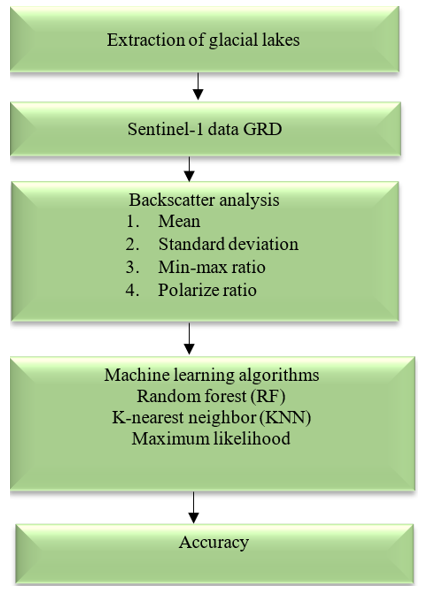
The GLs in this study were extracted using GRD data from SAR images. The goal was to properly categorize GLs using ML methods including RF, KNN, and Maximum Likelihood Classification (MLC). These algorithms were chosen because of their distinct capabilities in pattern recognition and categorization. GRD data, because of its sensitivity to surface features and ability to pierce cloud cover, is ideal for remote sensing applications in glaciated and mountainous areas. The ML models were trained on labeled data representing two basic classes lakes and glacier surfaces and then evaluated for classification accuracy. Using the spatial and backscatter information in the GRD data, these classifiers were able to discriminate between GLs and surrounding ice or snow-covered terrain with varied degrees of accuracy. Implementing these algorithms offered a robust and automated approach to GL mapping, which contributed to enhanced monitoring of cryospheric changes and prospective GLOF risk assessment shown in Figure 1.
Figure 1. Flow diagram of the proposed system
3.1 Dataset
The study was carried out in the Batura Glacier, which lies in the Karakoram Mountain Range of Gilgit Baltistan in northern Pakistan. The study site lies between approximately 36.45°N-36.65°N latitude and 74.45°E-74.85°E longitude, including the glacierized environment and its corresponding supraglacial lakes. The elevations in the study site vary from about 2500–7800 m above mean sea level. In the current study, Sentinel-1 GRD SAR images acquired on 15 August 2024 were utilized. These were captured in IW acquisition mode, dual polarization (Vertical Transmit-Vertical Receive (VV) and Vertical Transmit-Horizontal Receive (VH)), and ascending/descending orbit. The Sentinel-1 GRD SAR images have a spatial resolution of 10 m, and their imaging capacity is all-weather. The two polar-orbiting satellites that make up the Sentinel-1 mission employ C-band SAR to image at night and during the day. In enhanced SAR data, Level-1 GRD items are found. The GRD products' ellipsoidal projection is altered by the terrain height specified in the product general remark. The working terrain height is constant in range but varies in azimuth. Coordinates for the ground range are those that are projected onto the spheroid of the Earth. The observed magnitude is shown by the pixel values. Phase details are lost. The multi-look technique results in reduced speckle and almost square spatial resolution and pixel spacing. Using the thermal noise vectors included in the noise vector annotation data collection, which is a component of the product annotations, users may carry out a thermal noise correction by eliminating the noise from the power detected image. For example, the Sentinel-1 Toolbox (S1TBX) provides a function for thermal noise reduction. IW and EW GRD devices perform individual multi-origin on each burst. A single, continuous, ground-limit detected image is created by seamlessly combining the bursts from each polarization channel in each sub-square. The method of acquisition and the amount of multi-look used distinguish three resolutions of GRD products: full resolution (FR), high resolution (HR) and medium resolution (MR). Both polarizations of Sentinel-1 GRD data, that is VV and VH, have been used in this research. The use of the dual-polarization data has been made possible by the fact that the combination of VV and VH channels enhances the separability of GLs from ice- or snow-covered surfaces. In this study, 1055 pairs of co-registered VV-VH images were produced and pre-processed. The image pair includes the corresponding VV and VH backscatters from the same Sentinel-1 scene. Training samples were obtained from the manual delineation of lake and glacier surface areas on a pixel-by-pixel basis. In total, 10,000 pixels were labeled in this research. Half of them correspond to GLs and half of them to glacier surface classes shown in Table 1.
Table 1. Summary of the study area and datasets used in this study
|
Parameter |
Description |
|
Study Area |
Batura Glacier, Karakoram Range, Gilgit-Baltistan, Pakistan |
|
Geographic Coordinates |
36.45°N-36.65°N, 74.45°E-74.85°E |
|
Elevation Range |
Approximately 2500-7800 m above mean sea level |
|
Sentinel-1 Product Type |
Ground Range Detected (GRD) |
|
Acquisition Date |
15 August 2024 |
|
Satellite Mission |
Sentinel-1 |
|
Orbit Direction |
Ascending |
|
Imaging Mode |
Interferometric Wide Swath (IW) |
|
Polarization |
Dual polarization (VV and VH) |
|
Spatial Resolution |
10 m |
|
Number of Synthetic Aperture Radar (SAR) Images |
1055 co-registered VV–VH image pairs (VV + VH) |
|
Sentinel-2 Product |
Sentinel-2 Level-2A |
|
Sentinel-2 Acquisition Date |
18 August 2024 |
|
Cloud Condition |
Cloud-free (<10% cloud cover) |
|
Reference Data Source |
Sentinel-2 imagery, Google Earth imagery, and manual interpretation |
|
DEM Source |
Shuttle Radar Topography Mission (SRTM) DEM |
|
SRTM Spatial Resolution |
30 m |
3.2 Preprocessing
We used the real orbit data to guarantee accurate geolocation of Sentinel-1 VV GRD images. Boundary noise artifacts were eliminated to improve picture clarity, and thermal noise was decreased to improve signal quality. After that, radiometric calibration was used to transform the unprocessed SAR data into backscatter coefficients. To decrease speckle noise while preserving image features, the backscatter images were filtered using a Lee Sigma filter with a 3 × 3 window. Terrain correction was used to account for geometric aberrations using the SRTM 1-second HGT dataset. The adjusted SAR backscatter pictures were then converted to decibel (dB) scale for simpler comprehension. As an optical reference, Sentinel-2 imagery was used, specifically Level-2 Bottom-of-Atmosphere (BOA) corrected reflectance products with cloud cover below 10%. Sentinel-1 and Sentinel-2 datasets were co-registered using a common coordinate grid and amplitude normalization to ensure spatial alignment. The GLs and glacier surface class references were created manually using visual interpretation of clear Sentinel-2 L2A satellite images with the help of high-resolution Google Earth imagery and knowledge about the study area. The manually outlined polygons were then translated into pixel-based reference data for classifier training and validation. Both Sentinel-1 GRD images from 15 August 2024 and Sentinel-2 L2A images from 18 August 2024 were chosen to keep temporal consistency in both SAR and optical acquisitions. In order to avoid possible errors associated with seasonal differences in lake extent, snow coverage, and glacier activity, the time gap between the two datasets was kept under three days. The 1055 pairs of uint16-formatted images in the dataset were first cropped to 320 × 320 pixels and then scaled to 224 × 224 pixels to ensure compatibility with the model input. The names for GLs and glacier surfaces have been labelled using a visual interpretation process that relies on cloud-free Sentinel-2 Level-2A satellite images, along with Google Earth imagery, which is HR and based on previous knowledge of the region. These manual interpretations were then transformed to pixel samples that would train the ML models. The data preprocessing for Sentinel-1 GRD SAR images involved the use of the Sentinel Application Platform, which was produced by the ESA. In the beginning, the procedure of precise orbit correction was performed to increase the geometric accuracy of the SAR images. Then, the process of thermal noise removal was carried out to remove the additive noise that exists in the original GRD images. Radiometric calibration was then applied to transform the digital numbers into the backscatter coefficients (σ0). For the reduction of speckle noise and retention of important image characteristics, the Lee Sigma speckle filter (window size 3 × 3) was used throughout the research. Afterward, the process of Range-Doppler terrain correction was performed using the SRTM DEM (resolution 30 m). Bilinear interpolation was used as the resampling method during the process of terrain correction. Lastly, the transformation into dB using the logarithm of calibrated backscatter coefficients was done. After data preprocessing, the statistical backscatter features, such as mean, standard deviation (SD), minimum, maximum, Max-Min ratio, and Polarization Ratio (PR) were extracted from both VV and VH polarizations using 3 × 3 window size.
3.3 Feature extraction
Our research method involves the identification of two infrared polarizations: VH and VV, as well as calibration of GRD data using SAR infrared analysis. The polarization channels were analyzed using some backscatter estimators. Estimators detected by SNAP include PR, max-min ratio, mean, SD for VH and VV. Here are some of the formulas of these assessors.
3.3.1 Standard deviation
The total number of pixels in the local window is denoted by by $N$, and the backscatter coefficient of the $i^{t h}$ pixel is denoted by $\sigma_i$.
$stdev=\sqrt{\frac{1}{N} * \sum_{i=1}^N\left(10 \log _{10} \sigma_i\right)^2-\left(\frac{1}{N} * \sum_{i=1}^N 10 \log _{10} \sigma_i\right)^2}$ (1)
where, $N$ is the total number of pixels in the local window and $\sigma_i$ is the backscatter coefficient of the $i^{t h}$ pixel.
$S D=\sqrt{\frac{1}{N} \sum_{i=1}^N\left(x_i-\mu\right)^2}$ (2)
where, Eq. (2) represents N-number of pixels in the local window, $x_i$-backscatter value of pixel i, $\mu$-mean backscatter value.
3.3.2 Maximum-minimum ratio
The ratio of the two estimators is taken into consideration for the full execution of the maximum (VH and VV) and minimum (VH and VV).
$\max -\min$ ratio $=10 \log _{10}\left(\frac{\sigma^0 \operatorname{Max}}{\sigma^0 \operatorname{Min}}\right)$ (3)
where, Eq. (3) represents Max and Min are the max and min backscatters in the local window, respectively, while ε is some small value that avoids dividing by zero.
$\begin{array}{r}\sigma^0 \max -\text {sigma} 0 \text {Maxmium band} \sigma^0 \min - \text { sigma } 0 \text { Minband }\end{array}$
3.3.3 Polarization ratio
The PR was calculated using Eq. (4).
$\sigma^0 V H r V V=\left(\frac{\sigma^0 V H}{\sigma^0 V V}\right)$ (4)
where, VV and VH are the Sentinel-1 vertical transmit-vertical receive and vertical transmit-horizontal receive backscatters, respectively.
Statistical backscatter features for each pixel sample were computed for the VV and VH polarizations. Mean ($\mu$) and SD ($\sigma$) were computed in a local window to extract the distribution and textures. Minimum3 and Maximum3 were the minimum and maximum backscatter values obtained in a 3 × 3 window around the target pixel, respectively. The Max-Min ratio is computed as the ratio between the maximum and minimum backscatter values in the local window. PR was computed as the ratio of VV backscatter to VH backscatter as:
$\mathrm{PR}=\frac{V V}{V H}$ (5)
where, Eq. (5) represents (VV) and (VH) were the backscatter values of the respective Sentinel-1 polarization channels. All the computed features were normalized in the range [0, 1] before classification. The mathematical expression is shown in Table 2.
Table 2. Description of statistical backscatter features extracted from Sentinel-1 SAR data
|
Feature |
Equation |
Description |
|
Mean Backscatter |
$\mu=\frac{1}{N} \sum_{i=1}^N x_i$ |
It represents the mean SAR backscatter. intensity in a (3 × 3) window. |
|
SD |
$\sigma=\sqrt{\frac{1}{N} \sum_{i=1}^N\left(x_i-\mu\right)^2}$ |
It measures the variability and texture in SAR backscatter intensities. |
|
Minimum3 |
$\operatorname{Minimum}_3=\min \left(x_i\right), i=1, \ldots, N$ |
It represents the minimum backscatter intensity in a (3 × 3) window. |
|
Maximum3 |
$\operatorname{Maximum}_3=\max \left(x_i\right), i=1, \ldots, N$ |
It represents the maximum backscatter intensity in a (3 × 3) window. |
|
Max-Min Ratio |
$M M R=\frac{\operatorname{Maximum}_3}{\operatorname{Maximum}_3+\varepsilon}$ |
Local contrast enhancement of supraglacial lakes from the surroundings. Here, $\varepsilon$ is a small constant to avoid division by zero. |
|
PR |
$P R=\frac{\sigma_{V V}^0}{\sigma_{V H}^0}$ |
Ratio of VV to VH backscatter intensities for water body detection. |
3.4 Machine Learning classifiers
3.4.1 Random Forest
One bagging technique for decision trees is RF. A bootstrap training set of the same size is used to train decision trees. The optimal split variable is selected in each split step of decision tree training using a subset of m 0 features out of m features. The RF model's forecast is the sum of each decision tree's projections, depending on the number of votes. Specifically, the RF forecast is the label that receives the most votes.
Since we set nd = 200 in this instance, the RF has 200 decision trees. We establish m 0 = b√mc. Additionally, when training each decision tree, the frequently used Gini function is employed as the function to gauge the quality of a split. The definition of the Gini function is as follows, with pi representing the sample probability of class I in each group following the split:
$Gini =1-\sum_{i=1}^c\left(p_i\right)^2$ (6)
where, Eq. (6) represents $p_i$ is the probability of samples belonging to class i. Balanced sample weights are used to train the RF. The input data's class frequencies have an inverse relationship with the balanced sample weights.
The RF classifier is realized in this work with the number of trees being equal to 200 (nd = 200). The number of variables to be tested at each node is set to the square root of the total number of input variables (m' = √m). The Gini impurity was calculated according to Eq. (4) is selected as the splitting rule for the node and balanced sample weights are applied as a measure to resolve the problem of class imbalance. Tree depth restriction is not applied, allowing to grow trees to their maximum.
3.4.2 K-Nearest Neighbour
The KNN algorithm is a key component of the KNN method, which is one of the top five data mining approaches. The final output is a set of spatial points, which assumes that each feature in our training set represents a unique dimension at some location, and that the value of each observation for that feature corresponds to its coordinate. Therefore, we can use any suitable measure to estimate how similar two locations are based on their distance in this space. To determine which training set points are comparable enough to be taken into account when deciding which class to predict for a new observation, this method selects the data points closest to k due to its fast execution and ease of use. In this study, the Euclidean distance measure is used to calibrate KNN classifier. In order to use KNN classifier, all backscatter features are normalized to [0, 1] interval with the help of the min-max normalization method. The number of nearest neighbours is defined as k = 5, and Euclidean distance is used as the measure of similarity for finding the neighbourhood of each sample. The Euclidean distance was computed using Eq. (7), the distance between input vectors is thus found,
$D_{l j}=\sqrt{\sum_{k=1}^n\left(x_{i k}-x_{j k}\right)}$, for $k=1,2,3, \ldots$ (7)
For each data point in the dataset, the Euclidean distance between a new and current point is determined. After these separations are arranged in ascending order, the k elements with the smallest separations for the new point are selected. Once the classifier determines which of these elements is the dominant class, it resets it as the class for the newly found point. If a big enough k is chosen, KNN may effectively capture complicated and nonlinear patterns in the data while being resistant against noise and outliers. It does not need to be retuned or retrained; therefore, it is also quickly updated with fresh data.
3.4.3 Maximum Likelihood Classification
The threshold value for every class in MLC is derived from the training datasets (signature). Training signatures for the MLC Classifier are derived from the manually labelled samples of pixels representing GL and glacier surfaces. It is assumed that class statistics are distributed normally and the probability of each pixel belonging to one of the classes is computed based on the estimated mean vector and covariance matrix for each class.
A pixel's likelihood of belonging to a certain class is determined by the classifier based on the threshold value. Based on the highest likelihood of the assigned class, each pixel is categorized into a certain class.
The water pixels in this categorization are determined by:
In order to have a comparative analysis among the three classifiers used, the training and test datasets for the RF, KNN, and MLC algorithms consisted of the same input variables with a 70/30 ratio. The RF classifier used 200 decision trees, while the Gini index was adopted for splitting the nodes. The KNN algorithm used k = 5 along with Euclidean distance. And the MLC classifier used Gaussian distribution class signatures. The performance of the classifiers was measured using a wide range of class-level and total performance measures, including overall accuracy, precision, recall, F1-score, specificity, Kappa statistic, and error rate. Confusion matrices were created for all the classifiers to determine the discrimination ability of the classes in terms of GLs and glacier surface. Precision, recall, and F1-score were used to evaluate the GL class for measuring the accuracy of extracting GLs. Accuracy indicates the proportion of correct classifications, while precision and recall indicate the correctness and completeness of the GL classification, respectively. The harmonic mean of precision and recall is known as F1-score while specificity refers to the ability of the classifier to correctly classify non-class samples. The Kappa statistic is used to measure the agreement between the predicted and actual labels. As only a single polygon-level 70%/30% train/test split ratio was used, cross-validation and repeated experimentation were not conducted.
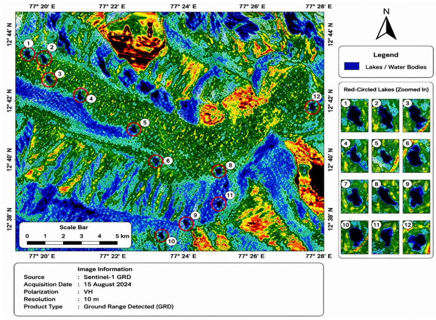
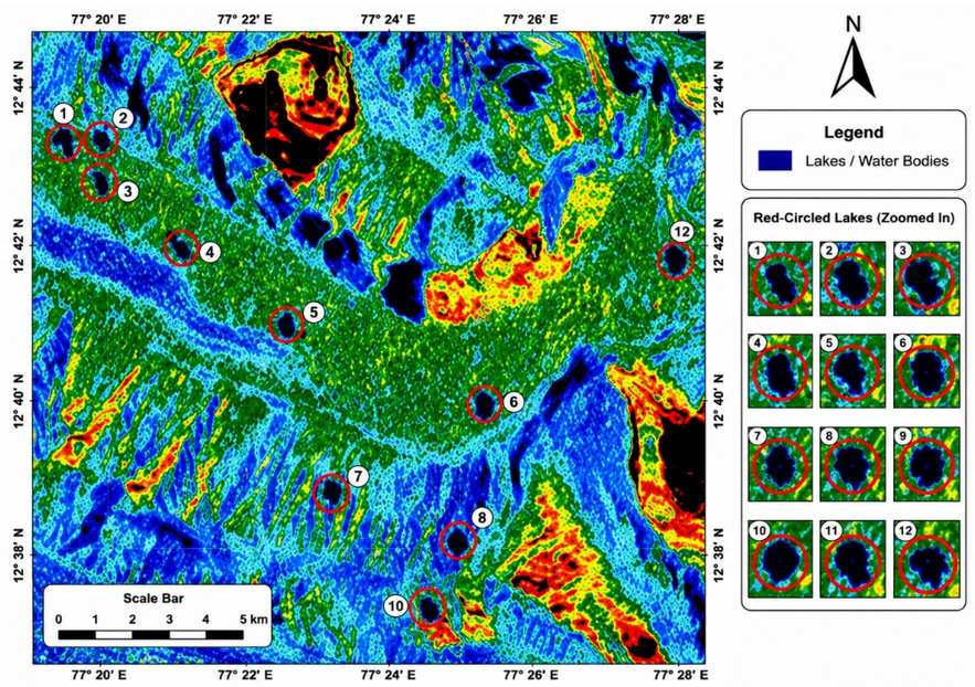
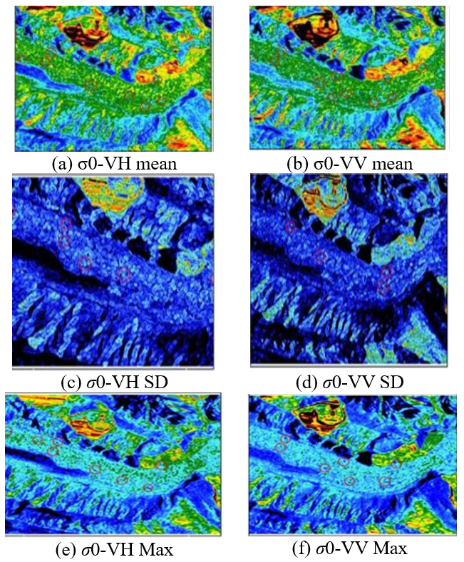
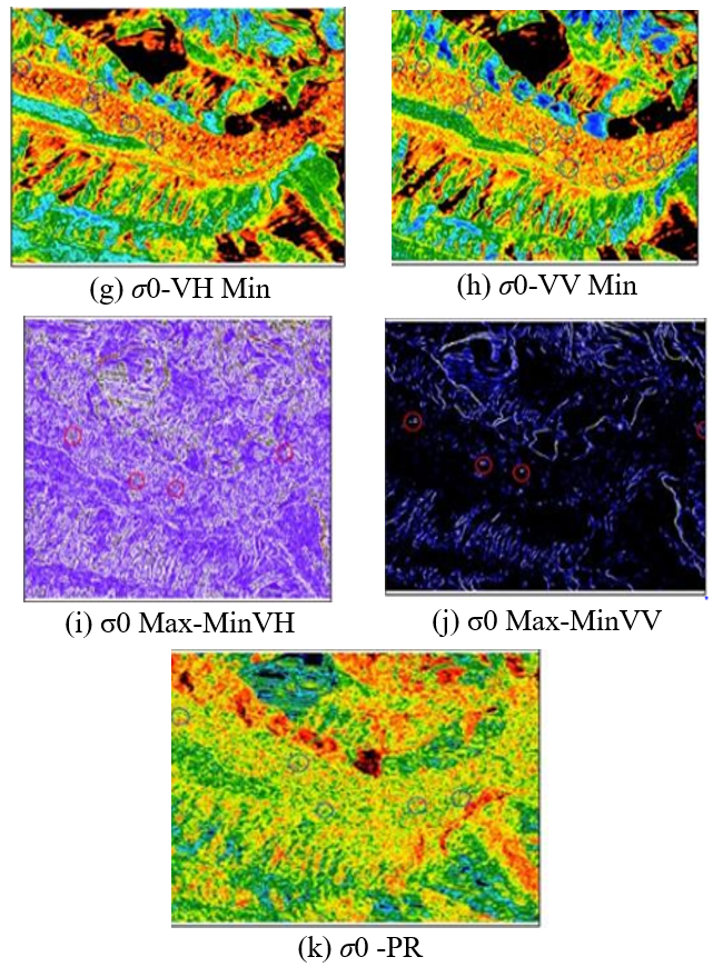
σ0-VH and σ0-VV are the two main polarized backscatter bands that are produced by the backscattering process following radiometric calibration of the GRD data. Both bands were subjected to a Lee Sigma filter (3 × 3 window) in order to reduce speckle noise and improve image clarity. By improving the visibility of surface characteristics, this filtering procedure makes it possible to identify GLs with greater accuracy. The glacier lakes on the Batura Glacier's surface are marked with red circles, as shown in Figures 2 and 3. The water bodies identified by the variations in the backscatter strengths of the VH and VV polarizations are highlighted by these circles.
For ensuring spatial independence between training and test datasets, the pixel samples obtained from the manual delineation of a particular lake or glacier polygon were allocated entirely to either the training or test dataset. Thus, neighbouring pixels that came from the same manual reference polygon were not contained in both training and test datasets. Even though an independent validation scene captured on a different date was not used in this study, future studies will explore the use of multi-date and independent scene validation approach.
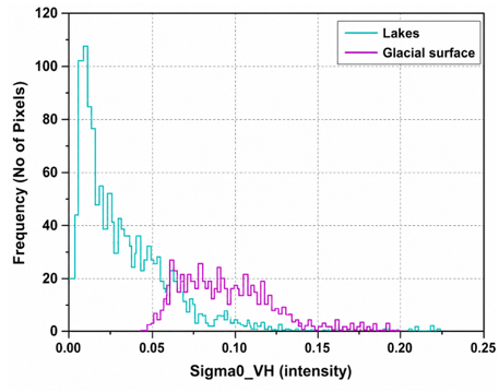
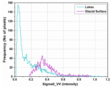
As seen in Figure 4 and Figure 5, the intensity levels of glacier lakes range from 0.05 to 0.15 for VH and from 0.2 to 0.6 for VV.
Mean backscatter analysis was performed to analyse the intensity properties of both the VH and VV polarizations with the use of a 3 × 3 moving window size. Figure 6(a) and Figure 6(b) show the mean backscatter of VH and VV polarizations, respectively. Apart from mean backscatter, SD was also used to describe the texture properties within SAR images. However, as indicated in Figure 6(c) and Figure 6(d), the SD property could not discriminate between the two features due to their similar backscatter property. Figure 6(e) and Figure 6(f) represent the maximum backscatter value while Figure 6(g) and Figure 6(h) indicate the minimum backscatter of the VH and VV polarizations. The max-min ratio is shown in Figure 6(i) and Figure 6(j), which improves the separation between water and glacier based on local backscatter contrast. Lastly, Figure 6(k) indicates the PR feature that distinguishes the GLs efficiently.
Figure 2. σ0 backscatter image of Vertical Transmit-Horizontal Receive (VH) polarization
Figure 3. σ0 backscatter image of Vertical Transmit-Vertical Receive (VV) polarization
Table 3. Classification results for performance metrics of Random Forest (RF), K-Nearest Neighbour (KNN), and Maximum Likelihood Classification (MLC) classifiers
|
Classification Algorithms |
Accuracy (%) |
Precision (%) |
Recall (%) |
F1-Score (%) |
Specificity (%) |
Kappa Coefficient |
Error Rate |
|
RF |
96 |
94 |
85 |
89 |
97 |
0.92 |
0.04 |
|
KNN |
93 |
97 |
92 |
94 |
94 |
0.89 |
0.07 |
|
MLC |
90 |
93 |
82 |
87 |
91 |
0.84 |
0.10 |
Figure 4. Performance of lakes in backscatter polarization
Figure 5. Performance of glacial surfaces in backscatter polarization
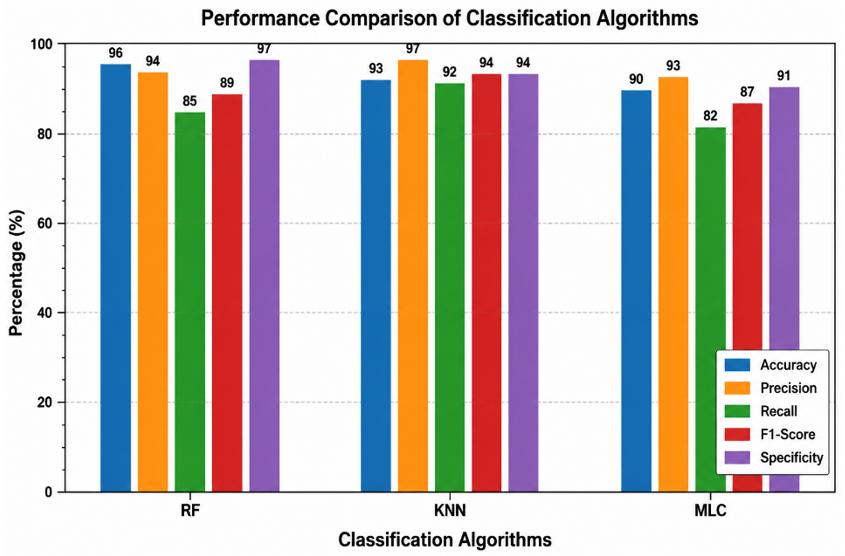
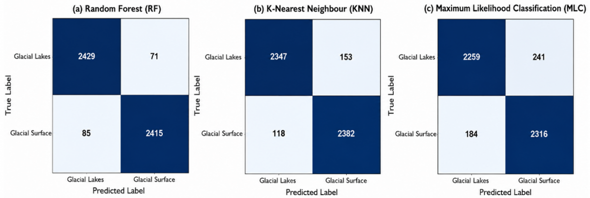
Supervised classification techniques require training samples that are representative of all relevant classes. Lakes and glacier surfaces where the two main classes for which training samples were gathered for this investigation. In total, 10,000 labelled pixels were extracted from manually annotated areas. They include 5,000 pixels of GLs and 5,000 pixels of glaciers' surfaces. The samples created based on the pixel approach were split between training (70%) and testing (30%) datasets on the polygon level to guarantee spatial independence between them. If the sample was collected from the manually outlined lake or glacier polygon, it could not be used in both the training and testing datasets because it would be included either in the training or testing dataset but never in both. In order to avoid spatial dependence between the two datasets for training and testing, the samples were stratified at the polygon level, as opposed to randomly sampling the polygons from the same image areas. Only one of each manually digitized GL or glacier polygon could be included in either the training or the testing dataset. Consequently, 3,000 samples were utilized for testing and validation, and 7,000 samples were used to train the classification models. Three particular classifiers were used in this investigation: MLC, KNN, and RF. Because it aggregates numerous decisions trees and provides better stability than a single decision tree, the RF classifier was chosen for its resilience in managing outliers. Because of its simplicity, ease of use, and benefit of not requiring a lot of training before generating predictions, KNN was selected. Lastly, because of its scalability and ability to function well with a high number of variables and data points, the MLC classifier was used. Table 3 provides a summary of each algorithm's categorization accuracy results and Figure 7.
In Figure 8, the confusion matrices of RF, KNN, and MLC are shown. These matrices give a class-by-class analysis of the performance of the classification algorithms. Out of all the classifiers, RF performed the best by having the highest number of classified samples.
Figure 6. Backscatter feature analysis of Vertical Transmit–Horizontal Receive (VH) and Vertical Transmit–Vertical Receive (VV) polarizations using a 3 × 3 moving window
Figure 7. Performance analysis of Random Forest (RF), K-Nearest Neighbour (KNN), and Maximum Likelihood Classification (MLC) classifiers
Figure 8. Confusion matrix analysis for Random Forest (RF), K-Nearest Neighbour (KNN), and Maximum Likelihood Classification (MLC) models used for GL extraction
This work shows how well Sentinel-1 GRD SAR data, in conjunction with statistical and ML classifiers, may be used to extract glacier lakes in hilly and cryospheric areas. Because of their continuously low radar returns, water bodies may be reliably identified using VV and VH backscatter analysis. The RF, KNN, and MLC methods were analysed, and the results showed that RF produced the best accuracy of 96%, KNN had an accuracy of 93%, and MLC produced an accuracy of 90%. This shows that the performance of RF is good in handling SAR backscatters in mountainous regions. The findings confirm that SAR-based lake detection is a valuable alternative to optical methods, especially under persistent cloud cover or in regions with limited daylight. Further work will focus on the use of multi-temporal SAR data and the addition of other types of optical imagery along with deep learning methods to enhance GL mapping accuracy and application.
No participation of humans takes place in this implementation process.
Human and Animal Rights: No violation of Human and Animal Rights is involved.
Competing Interests: The authors declare that they have no known competing financial interests or personal relationships that could have appeared to influence the work reported in this paper.
Funding: No funding was received for this study.
Availability of Data and Materials: The datasets are available from the corresponding author on reasonable request.
Maheswaran T led the research design, data preprocessing, and development of the Machine Learning models for automatic GL extraction using Sentinel-1 GRD SAR data. He also handled the implementation and performance evaluation of the classifiers. Cyril Mathew O contributed to data acquisition, feature engineering, validation of results, and preparation of the manuscript. Both authors collaboratively reviewed the outcomes, discussed findings, and finalized the paper for submission.
[1] Jiang, D., Li, X.W., Zhang, K., Marinsek, S., Hong, W., Wu, Y.R. (2022). Automatic supraglacial lake extraction in greenland using Sentinel-1 SAR images and attention-based U-Net. Remote Sensing, 14(19): 4998. https://doi.org/10.3390/rs14194998
[2] Tang, H.L., Lu, S.L., Baig, M.H.A., Li, M.Y., Fang, C., Wang, Y. (2022). Large-scale surface water mapping based on Landsat and Sentinel-1 images. Water, 14(9): 1454. https://doi.org/10.3390/w14091454
[3] Wangchuk, S., Bolch, T. (2020). Mapping of Glacial Lakes using Sentinel-1 and Sentinel-2 data and a random forest classifier: Strengths and challenges. Science of Remote Sensing, 2: 100008. https://doi.org/10.1016/j.srs.2020.100008
[4] Ali, S., Ali, S., Wang, L., et al. (2025). Deep learning model to detect Glacial Lakes using high-resolution optical and radar satellite images. Remote Sensing Applications: Society and Environment, 38: 101579. https://doi.org/10.1016/j.rsase.2025.101579
[5] Brun, F., Berthier, E., Wagnon, P., Kääb, A., Treichler, D. (2017). A spatially resolved estimate of High Mountain Asia glacier mass balances from 2000 to 2016. Nature Geoscience, 10: 668. https://doi.org/10.1038/NGEO2999
[6] Yao, X.J., Liu, S.Y., Han, L., Sun, M.P., Zhao, L.L. (2018). Definition and classification system of Glacial Lake for inventory and hazards study. Journal of Geographical Sciences, 28: 193-205. https://doi.org/10.1007/s11442-018-1467-z
[7] Rounce, D.R., Scott Watson, C., McKinney, D.C. (2017). Identification of hazard and risk for Glacial Lakes in the Nepal Himalaya using satellite imagery from 2000-2015. Remote Sensing, 9: 654. https://doi.org/10.3390/rs9070654
[8] Qayyum, N., Ghuffar, S., Ahmad, H.M., Yousaf, A., Shahid, I. (2020). Glacial lakes mapping using multi satellite planetscope imagery and deep learning. ISPRS International Journal of Geo-Information, 9(10): 560. https://doi.org/10.3390/ijgi9100560
[9] Chouksey, A., Thakur, P.K., Sahni, G., Swain, A.K., Aggarwal, S.P., Kumar, A.S. (2021). Mapping and identification of ice-sheet and glacier features using optical and SAR data in parts of central dronning maud land (cDML), East Antarctica. Polar Science, 30: 100740. https://doi.org/10.1016/j.polar.2021.100740
[10] Lu, Y.J., Zhang, Z., Kong, Y.R., Hu, K.H. (2022). Integration of optical, SAR and DEM data for automated detection of debris-covered glaciers over the western Nyainqentanglha using a random forest classifier. Cold Regions Science and Technology, 193: 103421. https://doi.org/10.1016/j.coldregions.2021.103421
[11] Chen, F., Zhang, M.M., Guo, H.D., et al. (2021). Annual 30 m dataset for Glacial Lakes in High Mountain Asia from 2008 to 2017. Earth System Science Data, 13(2): 741-766. https://doi.org/10.5194/essd-13-741-2021
[12] Wangchuk, S., Bolch, T., Robson, B.A. (2022). Monitoring Glacial Lake outburst flood susceptibility using Sentinel-1 SAR data, Google earth engine, and persistent scatterer interferometry. Remote Sensing of Environment, 271: 112910. https://doi.org/10.1016/j.rse.2022.112910
[13] Wu, R.Z., Liu, G.X., Zhang, R., et al. (2020). A deep learning method for mapping Glacial Lakes from the combined use of synthetic-aperture radar and optical satellite images. Remote Sensing, 12(24): 4020. https://doi.org/10.3390/rs12244020
[14] Zhang, M.M., Chen, F., Tian, B.S., Liang, D., Yang, A.Q. (2020). High-frequency Glacial Lake mapping using time series of Sentinel-1A/1B SAR imagery: An assessment for the southeastern Tibetan Plateau. International Journal of Environmental Research and Public Health, 17(3): 1072. https://doi.org/10.3390/ijerph17031072
[15] Wu, R.Z., Liu, G.X., Bao, X., et al. (2025). Eliminating geometric distortion with dual-orbit Sentinel-1 SAR fusion for accurate Glacial Lake extraction in Southeast Tibet Plateau. International Journal of Applied Earth Observation and Geoinformation, 136: 104329. https://doi.org/10.1016/j.jag.2024.104329
[16] Chen, F. (2021). Comparing methods for segmenting supra-Glacial Lakes and surface features in the mount everest region of the Himalayas using Chinese Gaofen-3 SAR images. Remote Sensing, 13(13): 2429. https://doi.org/10.3390/rs13132429
[17] Zhang, M.M., Chen, F., Guo, H.D., Yi, L., Zeng, J., Li, B. (2022). Glacial Lake area changes in High Mountain Asia during 1990-2020 using satellite remote sensing. Research, 2022: 9821275. https://doi.org/10.34133/2022/9821275
[18] Zhu, D.Y., Zhou, C.X., Zhu, Y.K., Wang, T., Zhang, C. (2023). Monitoring of supraglacial lake distribution and full-year changes using multisource time-series satellite imagery. Remote Sensing, 15(24): 5726. https://doi.org/10.3390/rs15245726
[19] Rinzin, S., Zhang, G.Q., Wangchuk, S. (2021). Glacial Lake area change and potential outburst flood hazard assessment in the Bhutan Himalaya. Frontiers in Earth Science, 9: 775195. https://doi.org/10.3389/feart.2021.775195
[20] Jiang, L., Lin, Z.Q., Zhou, Z.B., et al. (2024). Monitoring and disaster assessment of Glacier Lake outburst in High Mountains Asian using multi-satellites and HEC-RAS: A case of kyagar in 2018. Remote Sensing, 16(23): 4447. https://doi.org/10.3390/rs16234447
[21] Mondal, S.K., Patel, V.D., Bharti, R., Singh, R.P. (2023). Causes and effects of Shisper Glacial Lake outburst flood event in Karakoram in 2022. Geomatics, Natural Hazards and Risk, 14(1): 2264460. https://doi.org/10.1080/19475705.2023.2264460
[22] How, P., Messerli, A., Mätzler, E., et al. (2021). Greenland-wide inventory of ice marginal lakes using a multi-method approach. Scientific Reports, 11(1): 4481. https://doi.org/10.1038/s41598-021-83509-1
[23] Zhang, Y., Zhao, J., Yao, X.J., Duan, H.Y., Yang, J.X., Pang, W.L. (2023). Inventory of Glacial Lake in the southeastern Qinghai-Tibet Plateau derived from Sentinel-1 SAR image and Sentinel-2 MSI image. Remote Sensing, 15(21): 5142. https://doi.org/10.3390/rs15215142
[24] He, X.N., Zhang, S.C., Xue, B.W., Zhao, T., Wu, T. (2023). Cross-modal change detection flood extraction based on convolutional neural network. International Journal of Applied Earth Observation and Geoinformation, 117: 103197. https://doi.org/10.1016/j.jag.2023.103197
[25] Tang, H.L., Lu, S.L., Baig, M.H.A., Li, M.Y., Fang, C., Wang, Y. (2022). Large-scale surface water mapping based on Landsat and Sentinel-1 images. Water, 14(9): 1454. https://doi.org/10.3390/w14091454
[26] Zhao, X.R., Wang, X., Wei, J.F., Jiang, Z.L., Zhang, Y., Liu, S.Y. (2020). Spatiotemporal variability of glacier changes and their controlling factors in the Kanchenjunga region, Himalaya based on multi-source remote sensing data from 1975 to 2015. Science of the Total Environment, 745: 140995. https://doi.org/10.1016/j.scitotenv.2020.140995
[27] Avian, M., Bauer, C., Schlögl, M., et al. (2020). The status of earth observation techniques in monitoring high mountain environments at the example of Pasterze Glacier, Austria: Data, methods, accuracies, processes, and scales. Remote Sensing, 12(8): 1251. https://doi.org/10.3390/rs12081251
[28] Steffen, T., Huss, M., Estermann, R., Hodel, E., Farinotti, D. (2022). Volume, evolution, and sedimentation of future glacier lakes in Switzerland over the 21st century. Earth Surface Dynamics, 10(4): 723-741. https://doi.org/10.5194/esurf-10-723-2022