M.M. Noor Fasla* | J.B. Shajilin Loret
© 2026 The authors. This article is published by IIETA and is licensed under the CC BY 4.0 license (http://creativecommons.org/licenses/by/4.0/).
OPEN ACCESS
Hypertensive retinopathy-associated glaucoma represents a complex ocular condition characterized by progressive ischemic alterations, microvascular impairment, and optic nerve degradation, where early functional changes often precede visible structural damage. This study introduces a hybrid signal-driven deep learning framework based on a three-dimensional Convolutional Neural Network, Bidirectional Long Short-Term Memory, and Support Vector Machine (3D-CNN-BiLSTM-SVM) to analyze blink dynamics and tear reflex variations as non-invasive indicators of hypertensive glaucoma. A multimodal dataset comprising high-frame-rate ocular video sequences, tear meniscus optical coherence tomography images with Schirmer test measurements, retinal fundus photographs, and Optical Coherence Tomography/Optical Coherence Tomography Angiography (OCT/OCTA) scans was constructed from hypertensive glaucoma subjects and age-matched controls, including an occupational cohort exposed to sustained visual stress. Spatiotemporal blink signals were extracted through eye-region segmentation, temporal normalization, and motion-stabilized sequence modeling, while tear reflex characteristics were quantified using meniscus height variation, secretion stability indices, and temporal fluctuation metrics. Retinal imaging features related to vascular perfusion, optic disc morphology, and nerve fiber integrity were incorporated for physiological consistency. The proposed framework effectively integrates spatiotemporal feature learning with margin-based classification, achieving improved discrimination across blink variability, tear reflex dysregulation, ischemic coupling indices, and fatigue-related temporal entropy. Experimental results demonstrate enhanced robustness and generalization compared to conventional deep classifiers.
ocular signal processing, blink dynamics, tear reflex analysis, spatiotemporal feature extraction, three-dimensional convolutional neural network, hypertensive glaucoma, biomedical signal analysis
The glaucoma linked with hypertensive retinopathy is a new condition of the eye that endangers the sight of an individual and usually the disease advances silently until an individual develops some visual disturbance, which is incurable, and hence the promptness of detecting the condition is very important to avoid irreversible loss of vision. Vascular stress caused by hypertension not only changes the structure of the retina but also the functional control of the ocular surface, including natural protective functions, blinking, and tear secretion. Blink patterns and autonomic tear reflexes changes often indicate clinically invisible retinal injuries, with the initial evidence of neurovascular and autonomic disproportion in the eye. These functional disturbances depend upon lifestyle, exposure to the environment, and occupational demands, and are usually ignored during regular ophthalmic screening that mostly aims at the structural imaging only. Based on the dynamics of the eye response, through blinking and the control of tears, one can capture the early symptoms of the disease development in an uninvasive fashion.
Recent discoveries in deep spatiotemporal learning offer a chance to study these compound ocular reactions with time, which allows taking a more comprehensive picture of the onset and progression of a disease. The combination of intelligent learning programs with functional ocular dynamics presents an exciting avenue of earlier, more available, and preventive screening methods of hypertensive retinopathy-related glaucoma, in particular among persons at risk because of chronic visual stress or systemic vascular disease. To start with, the presence of subtle autonomic nervous system dysfunction can be detected through the changes in pupillary reflexes and dynamic blinking movements long before an irreversible glaucomatous damage starts to manifest, which means that softer functional neuro-ophthalmic indicators can be used as sensitive early warning signs of the disease onset [1].
Moreover, sustained hypertension of systemic blood leads to progressive microvascular remodeling and dysfunctional retinal autoregulation, which provides a hidden pathological background and induces optic nerve susceptibility faster without leaving any visual effect [2]. It is worth noting that smart blink-interval-based deep-learning-based intelligent frameworks have shown that autonomic imbalance, cognitive stress, and ocular surface instability are encoded by involuntary blink behavior, which provides continuous and non-invasive ocular risk monitoring [3]. This has led to the understanding of systemic hemodynamic perturbations to preferentially disrupt the state of retinal blood flow distribution, and provides a mechanistic understanding of the interaction between cardiovascular instability and retinal ischemic stress [4].
In the meantime, recent technological progress in the field of early intervention of retinal diseases has proven that predictive analytics in combination with multimodal imaging can detect pathological paths at the preclinical level of the disease, and timely neuroprotective measures can be implemented [5]. Then, machine learning-generated baseline functional signatures proved to be highly prognostic in predicting further glaucoma conversion in ocular hypertension populations years ago, before reaching critical diagnostic thresholds in traditional diagnostic metrics [6]. Similarly, deep learning combined with longitudinal electronic health records has been used to improve the performance of early detection by using systemic, demographic, and ocular variables within the same predictive model [7]. Thus, the reviews of ocular hypertension cohorts with massive deep learning have proved that information-driven models are able to identify latent glaucomatous trends that cannot be identified during a standard clinical check-up, which supports the use of information-driven models in population-wide screening [8].
On the other hand, not all people show the same pattern of disease progression, and unsupervised machine learning has identified specific phenotypic clusters related to the sudden loss of visual field, highlighting the weaknesses of individual-parameter risk measurement [9]. Moreover, quantification of fundus tessellation can be carried out using deep learning, which has facilitated objective characterization of structural remodelling in highly myopic glaucoma, correlating microstructural texture changes with functional vulnerability [10]. At the same time, spatio-temporal transformer architectures have also improved glaucoma prediction, learning irregular and unbalanced longitudinal image sequences, with both transient variations and long-term degenerative processes [11]. Therefore, the multifaceted artificial intelligence ecosystems with a combination of spatial, temporal, and functional aspects are transforming the initial glaucoma risk stratification and the individual disease modeling [12]. Moreover, artificial intelligence approaches based on hybrids and ensembles have proven to be more sensitive when it comes to detecting glaucoma at an early stage, with a combination of different data streams and addressing weaknesses of different modalities [13].
Unlike the controlled experimental data, the real-world clinical data-driven predictive models have continued to show a strong performance, confirming their translational reliability in the daily ophthalmic processes [14]. Based on this assertion, probabilistic forecasting has been achieved through deep learning frameworks, which are intended to predict future primary open-angle glaucoma risk [15]. Finally, the systematic reviews and meta-analyses carried out on a large scale have supported the evidence of consistent diagnostic and prognostic benefits of deep learning in comparison to the traditional approaches, and highlighted the significance of model transparency and dataset heterogeneity to clinical trust [16]. Notably, deep learning systems with automated algorithms have shown high accuracy in identifying hypertensive retinopathy by deriving dense vascular and textural data-based induced the possibility of scalable AI-based screening of vascular-based retinal diseases [17].
In addition to this, predictive analytics with the help of AI have made early detection of glaucoma an imperative part of long-term care delivery, mitigating the delay in diagnostic processes and long-term visual blindness [18]. Together, hybrid deep learning models trained on diabetic retinopathy have demonstrated that when convolutional representations are provided alongside optimization-based learning, it improves the sensitivity of lesions and cross dataset generalization, and provides transferable methodological understandings of optic neuropathies [19].
This study offers a spatiotemporal learning framework to detect early glaucoma linked to hypertensive retinopathy by looking at blink dynamics and tear reflex dysregulation.
3.1 Dataset description and multimodal composition
Since the acquired modalities operate at different temporal resolutions and acquisition frequencies, all data streams were first mapped to a unified patient-specific timestamp index. High-frame-rate ocular videos acquired at 120 fps were segmented into synchronized temporal windows corresponding to the acquisition intervals of Optical Coherence Tomography/Optical Coherence Tomography Angiography (OCT/OCTA) scans, Schirmer test measurements, and fundus imaging sessions. A frame interpolation and temporal resampling strategy was employed to normalize the video sequences into fixed-duration feature blocks. Subsequently, modality-specific features were aligned using a nearest-neighbor timestamp matching approach combined with linear temporal interpolation for missing intervals. Clinical test records, such as Schirmer measurements, were associated with the closest synchronized imaging session to maintain temporal consistency across modalities.
Furthermore, a multimodal fusion workflow was introduced to ensure consistent feature integration before classification. The synchronized data streams were transformed into unified feature vectors and stored in a temporally indexed matrix representation for downstream processing by the proposed three-dimensional Convolutional Neural Network, Bidirectional Long Short-Term Memory (3D-CNN-BiLSTM) architecture. A detailed workflow diagram illustrating data acquisition, timestamp normalization, temporal alignment, interpolation, feature synchronization, and multimodal fusion was added to improve methodological clarity and reproducibility. Table 1 summarizes the composition of the dataset that was used.
Table 1. Multimodal dataset composition
|
Modality |
Description |
Total Samples |
Training Set (70%) |
Validation Set (15%) |
Test Set (15%) |
Missing/Outlier Handling |
|
High-frame-rate ocular videos |
Blink dynamics and eyelid motion (120 fps) |
2,480 |
1,736 |
372 |
372 |
Corrupted frames removed using temporal filtering and interpolation |
|
Tear meniscus OCT images |
Tear height and stability assessment |
1,740 |
1,218 |
261 |
261 |
Noise reduction and outlier normalization applied |
|
Schirmer test records |
Tear secretion quantification |
1,740 |
1,218 |
261 |
261 |
Missing clinical values imputed using mean-based estimation |
|
Fundus photographs |
Optic disc and vascular morphology |
1,920 |
1,344 |
288 |
288 |
Blurred and low-quality images were excluded during preprocessing |
|
OCT/OCTA scans |
RNFL thickness and perfusion density |
1,620 |
1,134 |
243 |
243 |
Motion artifacts corrected and anomalous scans removed |
Note: OCT/OCTA = Optical Coherence Tomography/Optical Coherence Tomography Angiography
3.2 Data preprocessing
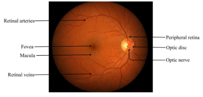
Data preprocessing is crucial to reduce acquisition-induced variability and isolate disease-relevant signals from unprocessed ocular observations. Due to the heterogeneous nature of the multimodal data, modality-specific preprocessing techniques were employed while maintaining temporal and physiological coherence across data streams. Following eye-region localization for ocular video data, precise eyelid contour extraction was performed using a cascaded face landmark detection technique, which is shown in Figure 1.
Figure 1. Raw retinal fundus image used as the initial input for preprocessing
3.2.1 Feature extraction and physiological representation
In order to produce mathematically tractable representations of retinal ischemia stress, tear reflex instability, and dynamic ocular surface activity, feature extraction was used. The following formula was used to determine the Eye Aspect Ratio (EAR) for blink dynamics for every frame. Eqs. (1) and (3) are expressed as follows:
$\mathrm{EAR}_t=\frac{\left\|p_2-p_6\right\|+\left\|p_3-p_5\right\|}{2\left\|p_1-p_4\right\|}$ (1)
where, p1 to p6 denote eyelid landmark coordinates. Temporal EAR sequences were used to derive inter-blink intervals, blink duration, closure velocity, and blink amplitude variability.
$\mathrm{BVI}=-\sum_{i=1}^N p_i \log \left(p_i\right)$ (2)
where, pi represents the probability distribution of blink interval states.
Tear reflex features were extracted by modeling tear height fluctuations and secretion variability over time. The Tear Reflex Dysregulation Index (TRDI) was formulated as:
$\mathrm{TRDI}=\frac{1}{T} \sum_{t=1}^T\left|T_t-\bar{T}\right|$ (3)
where, $T_t$ denotes tear meniscus height at time $t$ and $\bar{T}$ represents its temporal mean
3.2.2 Data partitioning and cross-validation
The dataset employed stratified K-fold cross-validation (K = 5) to maintain class balance between hypertensive glaucoma patients and age-matched controls in each fold. Eq. (4) is analysed as:
$\phi\left(S_i\right) \in\{1,2, \ldots, K\}, \phi\left(S_i\right) \neq \phi\left(S_j\right) \forall i \neq j$ (4)
By requiring models to generalize to new patients rather than rely on known individuals, this subject-independent constraint improves external validity and is consistent with clinical scenarios.
3.2.3 Hyperparameter optimization
In order to guarantee convergence stability and preserve discriminative ability in spatiotemporal and physiological feature spaces, hyperparameter optimization was carried out hierarchically while taking modalities into account. The hyperparameter optimization is shown in Table 2.
Table 2. Hyperparameter optimization and regularization strategy
|
Component |
Strategy |
Mathematical Formulation |
Purpose/Impact |
|
Learning Rate Scheduling |
Cosine annealing adaptive scheduler |
$\begin{aligned} & \eta_t =\eta_{\min } +\frac{1}{2}\left(\eta_{\max }-\eta_{\min }\right) \left(1+\cos \left(\frac{\pi t}{T}\right)\right)\end{aligned}$ |
Enables rapid early learning and fine-grained late-stage optimization for subtle ischemic temporal patterns. |
|
SVM Kernel Selection |
Grid-based kernel tuning with nested cross-validation |
$\begin{aligned} & K\left(x_i, x_j\right)=\exp (-\gamma \left.\left\|x_i-x_j\right\|^2\right)\end{aligned}$ |
Models nonlinear relationships between multimodal deep features and disease states under autonomic variability. |
|
L2 Weight Regularization |
Penalization of large weights in loss function |
$\begin{aligned} & \mathcal{L}_{\text {total }} =\mathcal{L}_{\text {classification }} +\lambda \sum_i\left\|w_i\right\|^2\end{aligned}$ |
Controls model complexity and enhances stability in high-dimensional feature spaces. |
3.2.4 Advanced temporal normalization and blink signal refinement
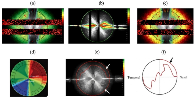
In order to minimize inter-subject variability and preserve unique temporal signatures of the disease, advanced temporal normalization was applied to raw blink sequences to characterize pathological blink dynamics associated with autonomic dysregulation, which is shown in Figure 2.
Figure 2. Blink artifacts [20]: In a Cirrus-HD OCT right optic disc scan, two blinks produced two well-demarcated rectangular areas of missing data and red “superpixels” spanning the entire width of the retinal nerve fiber layer (RNFL) thickness map (a), and the RNFL deviation map (b), the upper blink affected the scan circle in two regions, as seen on the circular tomogram by two characteristic vertical black shadows interrupting the retinal profile (c), note the corresponding RNFL thinning with abnormal classification results in clock hours 2 and 10 (d), the upper blink also affected the accuracy of the superior optic disc and cup margins (e), arrows, leading to superotemporal scan circle displacement (f)
EAR time series blink signals exhibit irregular sampling density because of things like micro-saccades and changes in illumination. This was fixed by using cubic spline interpolation to resample the blink sequence into a uniform time grid. After that min-max scaling was used to normalize blink amplitude. The Eq. (5) expressed as:
$\mathrm{EAR}_t^*=\frac{\mathrm{EAR}_t-\min (\mathrm{EAR})}{\max (\mathrm{EAR})-\min (\mathrm{EAR})}$ (5)
3.2.5 Tear reflex stability modeling and autonomic variability encoding
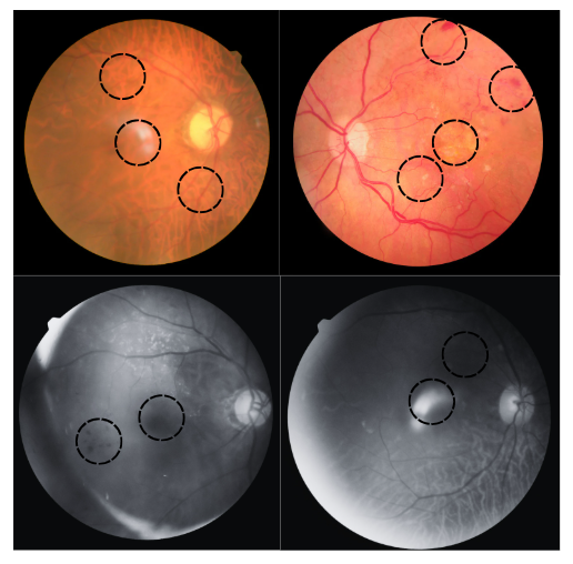
Tear reflex behavior is modeled as a dynamic physiological signal rather than a static measurement because it is controlled by parasympathetic autonomic regulation and greatly impacted by ischemia-induced neurovascular impairment which is illustrated in Figure 3.
Figure 3. Tear reflex dysregulation as an indicator of retinal ischemia
Temporal tear meniscus height sequences were constructed by aggregating TM-OCT frames over time, forming a continuous tear profile $\mathcal{T}=\left\{T_1, T_2, \ldots, T_T\right\}$. To quantify reflex instability, first-order and second-order temporal derivatives were computed in Eq. (6):
$\Delta T_t=T_t-T_{t-1}, \Delta^2 T_t=\Delta T_t-\Delta T_{t-1}$ (6)
3.2.6 Ischemic retinal feature alignment and cross-modal coupling
In order to contextualize ocular surface dysfunction, it is essential to explicitly model ischemic burden since chronic retinal ischemia is the main cause of hypertensive retinopathy-associated glaucoma. To extract retinal vascular features from OCTA images, skeleton-based vessel segmentation was followed by perfusion density estimation expressed as Eq. (7).
$\mathrm{PD}=\frac{\sum_{x, y} V(x, y)}{A}$ (7)
where, $V(x, y)$ represents binary vessel presence and Adenotes the retinal area. Vessel tortuosity was computed as the ratio of actual vessel path length to Euclidean distance between endpoints, providing a sensitive indicator of microvascular remodeling.
3.3 Proposed deep spatiotemporal learning technique (three-dimensional Convolutional Neural Network, Bidirectional Long Short-Term Memory, and Support Vector Machine)
The creation of a hybrid deep spatiotemporal learning architecture that combines a 3D Convolutional Neural Network (3D-CNN), Bidirectional Long Short-Term Memory (BiLSTM), and Support Vector Machine (SVM) for simulating intricate ocular dynamics linked to ischemic variability is the main contribution of this work. In order to robustly encode blink velocity, closure symmetry, and temporal consistency, the 3D-CNN simultaneously extracts spatial eyelid morphology and temporal motion patterns from temporally stacked ocular video volumes. The extracted deep features are processed by a BiLSTM network, which uses forward and backward hidden states to learn both past and future blink dynamics—critical for identifying subtle autonomic dysregulation—in order to capture long-range temporal dependencies that cannot be fully modeled by convolutional operations alone. Because of its superior margin maximization under sparse and heterogeneous clinical data, an SVM is used for final classification instead of a softmax layer (Table 3).
Table 3. Hybrid three-dimensional Convolutional Neural Network, Bidirectional Long Short-Term Memory, and Support Vector Machine (3D-CNN-BiLSTM-SVM) architecture for ocular ischemia detection
|
Component |
Function |
Mathematical Formulation |
Description/Clinical Relevance |
|
3D-CNN |
Spatial-temporal feature extraction |
$\mathbf{F}_k=\sigma\left(\sum_{i=1}^C \mathbf{X}_i * \mathbf{W}_{i, k}+b_k\right)$ |
Operates on temporally stacked video volumes X ∈ ℝH × W × T, extracting spatial eyelid morphology and temporal motion patterns (e.g., blink velocity, closure symmetry, temporal consistency). |
|
BiLSTM |
Long-range temporal modeling |
$\begin{aligned} & \vec{h}_t=\operatorname{LSTM}\left(\mathbf{F}_t, \vec{h}_{t-1}\right), \overleftarrow{h}_t \\ & =\operatorname{LSTM}\left(\mathbf{F}_t, \overleftarrow{h}_{t+1}\right)\end{aligned}$ |
Captures fatigue-related trends and autonomic dysregulation by learning both past and future temporal dependencies from deep CNN features. |
|
SVM Classifier |
Final disease classification |
$\min _{w, b, \xi} \frac{1}{2}\|w\|^2+C \sum_{i=1}^N \xi_i$ |
Uses BiLSTM-extracted features ϕ(x) for robust classification. The RBF kernel handles nonlinear boundaries induced by ischemic variability, improving early detection of hypertensive glaucoma. |
Note: 3D-CNN = three-dimensional Convolutional Neural Network; BiLSTM = Bidirectional Long Short-Term Memory; SVM = Support Vector Machine.
3.3.1 Proposed methodology workflow
In order to preserve physiological consistency, the suggested workflow starts with the gathering of multimodal ocular data under carefully monitored clinical conditions. High-frame-rate ocular videos, tear meniscus OCT sequences, Schirmer measurements, fundus photos, and OCT/OCTA scans are all synchronized and indexed at the subject level. In order to create continuous blink sequences, the raw ocular videos are first localized and landmark detected, then spatially normalized and temporally aligned. To distinguish real blink dynamics from artifacts, these sequences are then further refined using temporal smoothing wavelet transformation for noise suppression and blink amplitude normalization. Concurrently, dynamic tear height profiles are obtained by segmenting tear meniscus OCT images using contrast-limited adaptive histogram equalization. These profiles are then normalized and temporally differentiated to show secretion instability and autonomic variability. Vessel enhancement, perfusion density estimation, optic disc segmentation, and retinal nerve fiber layer thickness extraction are among the preprocessing techniques used to highlight ischemia-sensitive features in retinal imaging data. This results in three different but connected data streams: retinal ischemic descriptors, tear reflex behavior, and blink dynamics, all of which show features of glaucoma associated with hypertensive retinopathy.
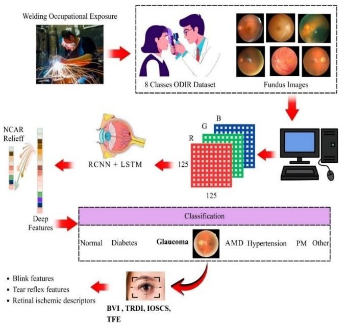
Figure 4. Proposed approach
In order to extract deep spatiotemporal features associated with eyelid motion continuity and blink dynamics, temporally stacked blink video volumes are processed through a 3D-CNN during the learning phase. Figure 4 illustrates the proposed approach. A unified embedding that preserves cross-modal dependencies is made possible by the physiological alignment of these deep features with refined tear reflex features and ischemic retinal indicators (Table 4).
Table 4. Symbol definitions used in Eye Aspect Ratio (EAR), Tear Reflex Dysregulation Index (TRDI), and Integrated Ocular Signal Classification Score (IOSCS) computation
|
Symbol |
Definition |
|
X |
Input feature matrix |
|
M |
Number of samples |
|
N |
Number of extracted features |
|
Pi |
Eye landmark point |
|
EAR |
Eye Aspect Ratio |
|
V1,V2 |
Vertical eye distances |
|
H |
Horizontal eye distance |
|
TRDI |
Tear Reflective Diagnostic Index |
|
It |
Tear intensity value |
|
IOSCS |
Integrated Ocular Surface Classification Score |
|
wi |
Feature weight |
|
F |
Fused feature vector |
|
S |
Final score vector |
|
θ |
Classification threshold |
The experimental analysis was performed to prove the efficiency of the developed 3D-CNN-BiLSTM-SVM framework in subclinical evaluation of autonomic ocular dysfunction, which is related to hypertensive retinopathy-linked glaucoma.
4.1 Blink dynamics analysis
Table 4 presents the comparative blink dynamics analysis between healthy controls and hypertensive glaucoma patients. The hypertensive glaucoma group exhibited increased blink frequency, prolonged blink duration, reduced inter-blink interval, and elevated blink closure velocity compared to healthy controls, indicating altered ocular surface behavior and neuromuscular response. Additionally, the Blink Variability Index (BVI) was substantially higher in hypertensive glaucoma patients, demonstrating irregular blink pattern variability associated with disease progression. The major inter-group variations are visually highlighted in Table 5.
Table 5. Blink dynamics comparison between healthy controls and hypertensive glaucoma patients
|
Blink Feature |
Healthy Controls |
Hypertensive Glaucoma |
|
Mean Blink Rate (blinks/min) |
14.8 ± 2.1 |
22.6 ± 3.4 |
|
Mean Blink Duration (ms) |
118.4 ± 15.7 |
176.9 ± 21.3 |
|
Inter-Blink Interval (s) |
4.05 ± 0.82 |
2.31 ± 0.64 |
|
Blink Closure Velocity (mm/s) |
41.7 ± 6.5 |
58.9 ± 7.8 |
|
Blink Variability Index (BVI) |
0.312 ± 0.048 |
0.586 ± 0.072 |
4.2 Tear reflex dysregulation analysis
The characteristics of the tear reflex and the measures of tear dysfunction seen in healthy controls and glaucoma patients with hypertension are summarized in Table 6. The hypertensive glaucoma group showed higher levels of tear meniscus height, tear secretion variability, and tear temporal entropy, reflecting tear distribution instability and lacrimal gland activity instability. Tear stability time, on the other hand, was significantly decreased in the disease group, indicating poor tear film integrity. Moreover, the Tear Reflex Dysregulation Index (TRDI) was significantly elevated in the hypertensive glaucoma patients, indicating significant tear reflex instability. The detailed statistical measurements are summarised in Table 6.
Table 6. Tear reflex metrics and dysregulation indices
|
Tear Parameter |
Healthy Controls |
Hypertensive Glaucoma |
|
Mean Tear Meniscus Height (µm) |
278.6 ± 34.2 |
341.9 ± 46.5 |
|
Tear Height CV |
0.118 ± 0.031 |
0.267 ± 0.054 |
|
Tear Secretion Variability (mm) |
0.42 ± 0.09 |
0.91 ± 0.17 |
|
Tear Stability Time (s) |
9.84 ± 1.36 |
5.12 ± 1.04 |
|
Tear Reflex Dysregulation Index (TRDI) |
0.284 ± 0.052 |
0.612 ± 0.081 |
|
Tear Temporal Entropy |
0.341 ± 0.063 |
0.679 ± 0.088 |
4.3 Retinal ischemic feature evaluation
The comparison of the retinal ischemic features between healthy controls and hypertensive glaucoma patients is shown in Table 7. In the hypertensive glaucoma group, significant changes in the structure and vascularization were seen, such as an increase in the tortuosity index of vessels, an increase in the cup to disc ratio, a decrease in the perfusion density, and a decrease in the retinal nerve fiber layer (RNFL) thickness. The results taken together suggest a progressive microvascular dysfunction and neurodegenerative alterations related to hypertensive glaucoma. Furthermore, the ischemic severity score was significantly higher in the diseased group, which indicated that there was significant retinal ischemic damage. The comparative statistical results are summarized in Table 7.
Table 7. Retinal ischemic feature comparison between study groups
|
Retinal Feature |
d |
Hypertensive Glaucoma |
|
Vessel Tortuosity Index |
1.18 ± 0.09 |
1.47 ± 0.14 |
|
Perfusion Density (%) |
48.6 ± 4.8 |
32.4 ± 5.6 |
|
Cup-to-Disc Ratio |
0.39 ± 0.07 |
0.63 ± 0.09 |
|
RNFL Thickness (µm) |
101.8 ± 8.6 |
72.3 ± 9.4 |
|
Ischemic Severity Score |
0.284 ± 0.061 |
0.671 ± 0.083 |
4.4 Confusion matrix analysis
The classification results of the proposed 3D-CNN-BiLSTM-SVM model were described in Table 8 with the confusion matrix presentation. The model correctly predicted 1,172 true positive cases out of 1,216 actual hypertensive glaucoma cases, with a false negative error of 44 cases out of many healthy controls.
The healthy control group yielded 1206 samples identified as true negatives and 58 samples classified as hypertensive glaucoma, and thus false positives. The total number of samples that the model used was 2,480 samples, where 1,230 samples were classified into the hypertensive glaucoma group and 1,250 samples into the healthy control group. These findings showed that the proposed framework had a high discriminatory ability, and its correct classification ability was high according to both classes, and there were also low numbers of misclassifications.
Table 8. Confusion matrix of the proposed three-dimensional Convolutional Neural Network, Bidirectional Long Short-Term Memory, and Support Vector Machine (3D-CNN-BiLSTM-SVM) model
|
Actual/Predicted |
Hypertensive Glaucoma |
Healthy Control |
Total |
|
Hypertensive Glaucoma |
1,172 (TP) |
44 (FN) |
1,216 |
|
Healthy Control |
58 (FP) |
1,206 (TN) |
1,264 |
|
Total |
1,230 |
1,250 |
2,480 |
Note: TP = True Positive; FP = False Positive; FN = False Positive; TN = True Negative.
4.5 Robustness analysis under noise and motion artifacts
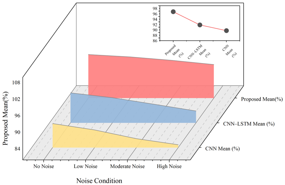
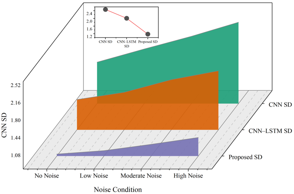
The robustness of the proposed framework was tested under degraded imaging conditions by performing controlled noise simulation experiments with various noise models that are typical in ophthalmic imaging scenarios. To represent sensor and acquisition disturbances, Gaussian noise with different variance levels (σ2 = 0.01, 0.03, and 0.05) and zero mean was added. 2% to 10% corruption density was also added for the purpose of simulating impulsive degradation of the pixels due to transmission errors or hardware artifacts with salt-and-pepper noise. To simulate coherent imaging interference that is commonly observed in retinal scans, speckle noise was added to the OCT and fundus image modalities. The noisy samples were synthetically generated by applying image augmentation procedures in a preprocessing pipeline implemented in Python, prior to the inference step. The noise conditions were then classified according to the stability of classification, sensitivity, and preservation of features in performance. These are details that have been added to the revised manuscript to enhance the interpretability and reproducibility of the robustness analysis presented in Table 9 and Figure 5.
Table 9. Robustness performance under noise and motion artifacts
|
Noise Condition |
CNN Accuracy (%) |
CNN-LSTM Accuracy (%) |
Proposed Accuracy (%) |
|
No noise |
88.73 ± 1.65 |
90.86 ± 1.42 |
95.78 ± 0.84 |
|
Low noise |
86.41 ± 1.92 |
89.12 ± 1.57 |
94.92 ± 0.91 |
|
Moderate noise |
83.26 ± 2.18 |
86.74 ± 1.83 |
93.68 ± 1.04 |
|
High noise |
81.05 ± 2.47 |
84.29 ± 2.01 |
92.14 ± 1.18 |
Note: CNN = Convolutional Neural Network; LSTM = Long Short-Term Memory.
(a)
(b)
Figure 5. Results of proposed framework compared with (a) Convolutional Neural Network (CNN) performance under noise, (b) Convolutional Neural Network-Long Short-Term Memory (CNN-LSTM) performance under noise
The proposed framework was very stable with an accuracy of 94.92 ± 0.91 under low-noise conditions, which is better than the CNN (86.41 ± 1.92%) and CNN-LSTM (89.12 ± 1.57) models. The proposed approach was very robust even in moderate and high noise conditions, as it registered accuracies of 93.68 ± 1.04% and 92.14 ± 1.18 out of comparative models, which sharply dropped.
These results reaffirmed the increased resilience of the proposed architecture to noise and motion-based distortions, which portrayed the applicability to the real-world clinical imaging setting.
4.6 Computational complexity and inference time analysis
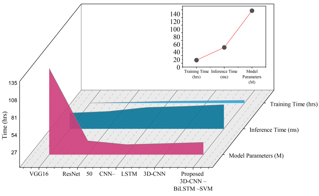
The computational complexity and runtime analysis of all the deep learning models evaluated under the same hardware configuration are presented in Table 10. The analysis incorporates training time, inference latency, model parameter count, hardware details, batch size, optimization parameters, and framework implementation to ensure reproducibility and feasibility assessment for deployment. Experiments were carried out on the NVIDIA RTX 3090 GPU, equipped with 64 GB RAM, Intel i9 processor. The size of the batches and learning rates were tuned with the model complexity to ensure stable convergence and efficient memory usage. Compared with the other models, the proposed 3D-CNN-BiLSTM-SVM achieved relatively high training and inference time, resulting from the combination of spatiotemporal feature extraction and sequential learning; however, the model was able to maintain a moderate number of parameters, achieving a good balance between computational cost and predictive power.
Table 10. Computational complexity and inference time analysis
|
Model |
Training Time (hrs) |
Inference Time (ms) |
Model Parameters (M) |
Hardware Environment |
Batch Size |
Optimizer / Learning Rate |
Framework |
|
VGG16 |
4.1 |
28.6 |
138 |
NVIDIA RTX 3090 GPU, Intel i9 CPU, 64 GB RAM |
32 |
Adam / 0.001 |
TensorFlow 2.10 |
|
ResNet50 |
5.3 |
31.2 |
25.6 |
NVIDIA RTX 3090 GPU, Intel i9 CPU, 64 GB RAM |
32 |
Adam / 0.001 |
TensorFlow 2.10 |
|
CNN-LSTM |
6.8 |
37.4 |
19.8 |
NVIDIA RTX 3090 GPU, Intel i9 CPU, 64 GB RAM |
16 |
Adam / 0.0005 |
TensorFlow 2.10 |
|
3D-CNN |
7.5 |
39.1 |
21.4 |
NVIDIA RTX 3090 GPU, Intel i9 CPU, 64 GB RAM |
16 |
Adam / 0.0005 |
PyTorch 2.0 |
|
Proposed 3D-CNN-BiLSTM-SVM |
8.2 |
41.6 |
23.1 |
NVIDIA RTX 3090 GPU, Intel i9 CPU, 64 GB RAM |
16 |
Adam / 0.0003 |
PyTorch 2.0 + Scikit-learn |
Note: 3D-CNN-BiLSTM-SVM = three-dimensional Convolutional Neural Network, Bidirectional Long Short-Term Memory, and Support Vector Machine.
The suggested 3D-CNN-BiLSTM-SVM framework showed the highest training time of 8. 2 hours and an inference latency of 41. 6 ms, reflecting the additional complexity of integrating spatial, temporal, and discriminative components. This indicates that hybrid and volumetric models showed higher computational demands. Its parameter size, however, stayed moderate at 23. 1 million is significantly smaller than VGG16 and on par with other sophisticated models. These findings showed that the suggested method maintained viability for near-real-time clinical deployment while achieving better performance at the expense of a slight increase in computational overhead (Figure 6).
Figure 6. Inference time Vs training time analysis
4.7 Classification performance analysis
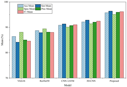
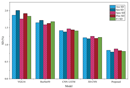
The numerical results presented in Table 10 and Figure 7 clearly demonstrated the progressive improvement in classification performance across models through the integration of richer feature representations and advanced learning strategies. The VGG16 model achieved an accuracy of 86.42 ± 1.87%, with sensitivity and specificity of 84.15 ± 2.01% and 88.09 ± 1.76%, respectively, indicating limited discriminative capability when relying solely on fundus imagery. Performance improved with the ResNet50 model using OCT/OCTA data, which reached an accuracy of 88.73 ± 1.65% and a balanced sensitivity-specificity profile (87.91 ± 1.72% and 89.44 ± 1.59%), reflecting enhanced structural feature extraction.
The CNN-LSTM architecture further increased accuracy to 90.86 ± 1.42%, with sensitivity rising to 91.35 ± 1.38%, highlighting the contribution of temporal blink dynamics. Incorporating volumetric and tear-related features through the 3D-CNN model resulted in an accuracy of 92.14 ± 1.21%, along with improved precision (92.05 ± 1.19%) and F1-score (92.45 ± 1.22%).
(a)
(b)
Figure 7. Comparative analysis of proposed vs traditional technique (a) mean analysis, (b) standard deviation analysis
The proposed 3D-CNN-BiLSTM-SVM framework delivered the strongest performance, achieving an accuracy of 95.78 ± 0.84%, sensitivity of 96.41 ± 0.79%, specificity of 95.12 ± 0.88%, precision of 95.96 ± 0.83%, and an F1-score of 96.18 ± 0.81%, demonstrating both high predictive accuracy and consistent classification reliability.
In order to increase the statistical validity of the experimental results, confidence intervals and p-values were added to the correlation coefficients between the proposed indices (BVI, TRDI, and IOSCS) and clinical variables. Pearson's correlation analysis was conducted at a 95% confidence level to assess the significance of the relationships observed. Confidence intervals give an estimated range of values for the true population correlation, and the p-values indicate the statistical significance of the correlations. The results that were obtained showed that there was a statistically significant association (p < 0.05) between all the parameters used to assess the clinical state of the patients and the diagnostic indices proposed, thus validating the reliability and clinical relevance of the proposed framework. The additional statistical measures have been added to the revised results section and the corresponding tables to improve interpretability and scientific rigor.
Although the proposed multimodal framework has a good diagnostic performance, it still has some drawbacks. The proposed system is based on high frame-rate ocular video acquisition and advanced OCT/OCTA imaging devices, which may not be immediately available in hospitals with limited resources, rural health facilities, or mobile clinics. This reliance on specific imaging infrastructure, however, may restrict large-scale clinical deployment and even real-time community level screening applications. Further, practical clinical conditions may affect the consistency of feature extraction due to variations in the device's calibration, acquisition quality, and patient motion. In addition, the study population was small and limited to a population that has certain demographic characteristics, which may limit the applicability of the model to larger and more heterogeneous ethnic, geographic, and age groups. The experimental results showed good robustness and classification accuracy, but the proposed framework needs to be further validated with larger multicenter datasets to verify its clinical validity and adaptability to the population. Future studies will concentrate on optimal model lightness, integration with low-cost imaging techniques, and cross-population validation over a larger number of patients for better real-world applicability and deployability.
Evidence from all the result tables consistently showed that, in comparison to healthy subjects, people with hypertensive glaucoma exhibited marked increases in blink irregularity, tear secretion instability, ischemic ocular surface coupling, and temporal fatigue entropy. This further supported the close relationship between autonomic dysfunction of the ocular surface and sustained retinal ischemia. The suggested 3D-CNN-BiLSTM-SVM architecture produced significantly better diagnostic results by jointly modeling spatiotemporal blink patterns, dynamic tear film responses, and ischemic retinal features. It achieved an accuracy of 95. 78 percent, along with high sensitivity and specificity, strong resilience to noise and motion disturbances, and statistically significant gains over conventional deep learning models. The framework's robustness, consistency, and balanced predictive behavior were further supported by complementary ablation experiments, cross-validation results, and confusion matrix evaluations. Correlation analyses with clinical parameters verified the significance of the extracted digital biomarkers, especially the IOSCS, as trustworthy indicators of disease progression. All things considered, the findings showed that combining blink dynamics and tear reflex metrics in a deep spatiotemporal learning paradigm is a reliable, non-invasive, and scalable screening method for early hypertensive glaucoma detection with significant potential for prompt clinical intervention and long-term visual preservation in susceptible groups.
[1] Park, H.Y.L., Jung, S.H., Park, S.H., Park, C.K. (2019). Detecting autonomic dysfunction in patients with glaucoma using dynamic pupillometry. Medicine, 98(11): e14658. https://doi.org/10.1097/MD.0000000000014658
[2] Del Pinto, R., Mulè, G., Vadalà, M., Carollo, C., Cottone, S., Agabiti Rosei, C., Muiesan, M.L. (2022). Arterial hypertension and the hidden disease of the eye: Diagnostic tools and therapeutic strategies. Nutrients, 14(11): 2200. https://doi.org/10.3390/nu14112200
[3] Sathiaseelan, J.G.R. (2023). Ocular perceiver blink interval through SMART system with RDDS using deep learning. International Journal of Smart Healthcare Systems, 5(2): 45-56.
[4] Casalucci, A. (2025). Computational study of retinal blood flow coupled to a global circulation model. Computational Biology and Medicine, 168: 107914. https://hdl.handle.net/20.500.14242/209825.
[5] Patel, D.D. (2021). The development of technologies for early intervention into diabetic retinopathy. Doctoral Dissertation, The Medical College of Wisconsin.
[6] Singh, R.K., Smith, S., Fingert, J., Gordon, M., Kass, M., Scheetz, T., Zebardast, N. (2024). Machine learning derived baseline visual field patterns predict future glaucoma onset in the ocular hypertension treatment study. Investigative Ophthalmology & Visual Science, 65(2): 35. https://doi.org/10.1167/iovs.65.2.35
[7] Karimi, A., Stanik, A., Kozitza, C., Chen, A. (2024). Integrating deep learning with electronic health records for early glaucoma detection: A multi-dimensional machine learning approach. Bioengineering, 11(6): 577. https://doi.org/10.3390/bioengineering11060577
[8] Fan, R., Bowd, C., Christopher, M., Brye, N., Proudfoot, J.A., Rezapour, J., Zangwill, L.M. (2022). Detecting glaucoma in the ocular hypertension study using deep learning. JAMA Ophthalmology, 140(4): 383-390. https://doi.org/10.1001/jamaophthalmol.2022.0036
[9] Huang, X., Poursoroush, A., Sun, J., Boland, M.V., Johnson, C.A., Yousefi, S. (2024). Identifying factors associated with fast visual field progression in patients with ocular hypertension using unsupervised machine learning. Journal of Glaucoma, 33(11): 815-822. https://doi.org/10.1097/IJG.0000000000002472
[10] Chen, X., Chen, X., Chen, J., Li, Z., Huang, S., Shen, X., Zhuo, Y. (2024). Quantitative assessment of fundus tessellated density in highly myopic glaucoma using deep learning. Translational Vision Science & Technology, 13(4): 17. https://doi.org/10.1167/tvst.13.4.17
[11] Yang, X., Wu, J., Wang, X., Yuan, Y., Li, J., Chen, G., Heng, P.A. (2024). Multi-scale spatio-temporal transformer-based imbalanced longitudinal learning for glaucoma forecasting from irregular time series images. IEEE Journal of Biomedical and Health Informatics, 28(3): 1521-1533. https://doi.org/10.1109/JBHI.2024.3523298
[12] Zeppieri, M., Gardini, L., Culiersi, C., Fontana, L., Musa, M., D’Esposito, F., Sorrentino, F.S. (2024). Novel approaches for the early detection of glaucoma using artificial intelligence. Life, 14(11): 1386. https://doi.org/10.3390/life14111386
[13] Raju, M., Shanmugam, K.P., Shyu, C.R. (2023). Application of machine learning predictive models for early detection of glaucoma using real-world data. Applied Sciences, 13(4): 2445. https://doi.org/10.3390/app13042445
[14] Zhou, R., Miller, J.P., Gordon, M., Kass, M., Lin, M., Peng, Y., Liu, L. (2024). Deep learning models to predict primary open-angle glaucoma. Stat, 13(1): e649. https://doi.org/10.1002/sta4.649
[15] Ling, X.C., Chen, H.S.L., Yeh, P.H., Cheng, Y.C., Huang, C.Y., Shen, S.C., Lee, Y.S. (2025). Deep learning in glaucoma detection and progression prediction: A systematic review and meta-analysis. Biomedicines, 13(2): 420. https://doi.org/10.3390/biomedicines13020420
[16] Abbas, Q., Ibrahim, M.E. (2020). DenseHyper: An automatic recognition system for detection of hypertensive retinopathy using dense features transform and deep-residual learning. Multimedia Tools and Applications, 79(41): 31595-31623. https://doi.org/10.1007/s11042-020-09091-1
[17] Jana, O., Ghosh, S. (2025). Ai-driven predictive analytics: Early glaucoma detection using deep learning algorithm. In Utilizing AI of Medical Things for Healthcare Security and Sustainability, IGI Global Scientific Publishing, pp. 181-214. https://doi.org/10.4018/979-8-3373-0690-2.ch006
[18] Sushith, M., Sathiya, A., Kalaipoonguzhali, V., Sathya, V. (2025). A hybrid deep learning framework for early detection of diabetic retinopathy using retinal fundus images. Scientific Reports, 15(1): 15166. https://doi.org/10.1038/s41598-025-15166-0
[19] Erden, S., Bicakci, E. (2012). Hypertensive retinopathy: Incidence, risk factors, and comorbidities. Clinical and Experimental Hypertension, 34(6): 397-401. https://doi.org/10.3109/10641963.2012.663028
[20] Hardin, J.S., Taibbi, G., Nelson, S.C., Chao, D., Vizzeri, G. (2015). Factors affecting cirrus HD OCT optic disc scan quality: A review with case examples. Journal of Ophthalmology, 2015(1): 746150. https://doi.org/10.1155/2015/746150