Aboubakr Missaoui | Fatima Chouireb | Boubakeur Latreche | Abdelkerim Souahlia | Abdelaziz Rabehi* | Mawloud Guermoui | Messaoud Linani | Amel Ali Alhussan | Doaa Sami Khafaga | Marwa M. Eid | El-Sayed M. El-Kenawy
© 2026 The authors. This article is published by IIETA and is licensed under the CC BY 4.0 license (http://creativecommons.org/licenses/by/4.0/).
OPEN ACCESS
Voice disorders represent a significant healthcare burden worldwide, affecting communication and quality of life. To address this issue, some recent research has turned to automated acoustic analysis, relying on the Gammatone spectrum which mimics human hearing. However, these studies did not use a comprehensive methodology to select the optimal parameters for generating these spectra. In this research paper, we present an automated system for detecting voice disorders through a structured, systematic framework that identifies the optimal parameters for Gammatone spectrograms, where audio signals are converted into grayscale visual representations. Our fundamental contribution lies in moving beyond mere parameter adjustment to selecting the best parameters and creating specialized auditory representations for the task of voice pathology detection. This study involved a comprehensive systematic analysis of frequency range, window length, overlap amount, number of filters, and color scale. The system was evaluated using data from the Saarbrücken Voice Database (SVD), where it achieved a detection accuracy of 88.44 ± 1.17, demonstrating the effectiveness of our optimization approach and highlighting the crucial importance of parameter selection for achieving optimal performance in clinical voice assessment.
acoustic signal processing, voice disorder detection, Gammatone spectrogram, parameter optimization, Convolutional Neural Network, SqueezeNet, deep learning, acoustic analysis, Saarbrücken Voice Database
Voice disorders represent a significant clinical challenge affecting millions worldwide, with diverse etiologies spanning organic, neurological, and functional origins [1]. Traditional diagnostic approaches primarily involve clinical evaluations, including laryngeal endoscopic examinations and auditory-perceptual assessments conducted by speech-language pathologists. While these methods are considered the clinical gold standard, they present limitations such as high costs, dependency on specialist expertise, and variable accuracy due to subjective interpretation [2]. Consequently, increasing attention is being paid to the development of automated, objective methodologies for vocal disorder assessment, aiming to provide reliable and consistent evaluations
Automatic acoustic analysis of the voice is based on the principle that any dysfunction in the human phonatory system, such as irregular vocal fold vibrations, leaves measurable imprints in the resulting audio signal. The relationship between the physiology of the vocal tract and the characteristics of the acoustic signal has been comprehensively documented in the scientific literature, forming the basis for both voice engineering and analysis [3].
While traditional spectral analysis methods are widely used to extract features from speech signals, recent research suggests that approaches inspired by the human auditory system may be more effective at detecting subtle irregularities associated with voice disorders. Gammatone spectrograms represent a computationally sophisticated model of human cochlear sound processing, where their resolution and response vary non-linearly across different frequencies in a way that mimics the human ear [4-6]. Recent studies have shown that features based on Gammatone filters are particularly effective in detecting and classifying voice disorders, even outperforming other fundamental features [3-8].
Despite these advancements, a significant research gap remains: current investigations lack a comprehensive systematic analysis of how fundamental parameters in spectrogram generation affect detection accuracy [7, 8]. To address this critical research gap, this study introduces an optimized framework for voice disorder detection that utilizes Gammatone spectrograms as visual input to a pre-trained SqueezeNet convolutional neural network [9].
This work presents four key contributions to the field of automated voice pathology detection: First, we introduce a Systematic Parameter Optimization Framework that identifies the optimal Gammatone spectrogram configuration through physiologically-guided analysis. Second, we develop an Integrated Detection System combining optimized spectrograms with an efficient deep learning architecture. Third, we provide a Practical Reference Framework with ready-to-use optimal parameters for researchers. Fourth, we conduct rigorous Cross-Gender and Statistical Robustness Validation, ensuring full statistical transparency and reliable performance across diverse populations.
The field of automatic voice disorder detection has evolved through several methodological stages. Initially, systems relied on the extraction of acoustic features such as Mel-frequency Cepstral Coefficients (MFCCs) [10, 11] and physiological characteristics like fundamental frequency (F0) and jitter [12, 13]. These features were then used as inputs for traditional machine learning classifiers like Support Vector Machines (SVMs) [14, 15] and Random Forests (RF) [16]. Although demonstrating effectiveness, these methods showed limitations in capturing complex vocal patterns, as evidenced by studies such as Verde et al. [17] achieved a binary accuracy of 85.77%, while Al-Dhief et al. [18] reached 81.48% in a similar task.
The advancement of deep learning has shifted focus toward spectrogram-based analysis, where audio signals are treated as visual inputs for Convolutional Neural Networks (CNNs) [8, 19] and Recurrent Neural Networks (RNNs) [20, 21]. In this context, researchers began exploring auditory-inspired spectral plots. For instance, the work of Zhou et al. [7] introduced innovative features called Gammatone Spectral Latitude (GTSL), which achieved an accuracy of 89.9%using traditional classifiers. However, this study provided limited statistical validation, lacking standard deviation measures and detailed performance analysis.
Research combining auditory-inspired representations with deep learning shows promise but reveals methodological considerations. For instance, Islam et al. [8] presented a different perspective using Cochleagrams as inputs to a VGG16 CNN, achieving a detection accuracy of 100% on a dataset of 200 voice samples, though the limited dataset size requires attention. Similarly, Arias-Vergara et al. [6] employed multi-channel spectral plots including Gammatone representations, achieving an F1-score of 0.84 using data from 107 Cochlear Implant users and 94 healthy speakers, with the sample size noted as a consideration.
Validation methodologies vary substantially across studies, ranging from fixed data splits (80%/20% [18, 22] or 75%/25% [23, 24]) to cross-validation approaches (10-Fold [17], 4-Fold). Computational requirements significantly influence methodological choices, with less complex classifiers typically employing cross-validation for statistical reliability. A notable concern involves inconsistent reporting of performance variability, as many studies omit standard deviation values [11, 17, 25], limiting assessment of result stability. Computationally intensive models such as deep CNNs [23, 24, 26] frequently utilize fixed data splits due to resource constraints, potentially affecting statistical assessment. Some studies demonstrate improved practices, as seen in Yagnavajjula et al. [27], who reported both mean and standard deviation for 10-Fold cross-validation results.
While existing research establishes the value of deep learning and auditory-inspired spectrograms, a significant research gap remains regarding systematic parameter optimization for spectrogram generation in voice pathology detection. This study addresses this gap through comprehensive parameter analysis while maintaining statistical rigor via 5-Fold cross-validation with complete performance metrics reporting.
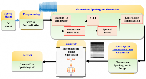
Figure 1 illustrates the complete workflow of the proposed system, from audio signal acquisition to the classification of voice disorders.
The proposed system utilizes a multi-stage methodology for detecting voice disorders. This approach centers on converting raw audio signals into information-rich visual representations (Gammatone spectrograms), which subsequently serve as inputs to a deep learning model designed for visual classification. The following sections describe each stage of this processing and analysis pipeline in detail.
Figure 1. Flowchart of the proposed system in voice pathology detection
3.1 Database
The study, in its detection phase, relied on the Saarbrücken Voice Database (SVD), which is considered an important reference in voice pathology research due to its rich diversity. This collection is distinguished by providing a wide variety of voice recordings for both healthy and pathological individuals, along with precise clinical details. It also includes speakers of both genders and various age groups, making it a valuable resource for building robust diagnostic systems.
To focus on voice disorders with complex or unknown etiologies (e.g., inflammations, tumor diseases, and neurological disorders), Thus, we excluded cases with clear and specific causes, such as those resulting from accident-related injuries (e.g., endotracheal tube damage) or surgical resections. The final dataset included 522 healthy voice samples (304 female and 218 male) and 585 pathological samples (277 female and 308 male), resulting in a total of 1107 samples. These pathological samples were classified into 15 distinct subcategories, reflecting the great diversity of the complex voice disorders that were analyzed.
3.2 Pre-processing
The audio signals were processed according to the following steps to ensure the quality and reliability of the data input into the spectral analysis system. This study focused on analyzing the acoustic properties of the sustained vowel /a/, a choice attributed to several factors: the vocal stability it provides, its ease of pronunciation for most individuals, and its widespread use as a standard in pathological voice assessment protocols [28].
To ensure the analysis is confined to the relevant vocal segments, the following steps were applied:
(1) Voice Activity Detection (VAD) and silent Removal: An algorithm was employed to identify and remove silent segments or non-vocal noise from the beginning and end of each recording. This algorithm relied on energy thresholds [29] to ensure that subsequent analysis focused exclusively on the active voice portion of the signal.
(2) Signal Amplitude Normalization: The amplitude of each processed audio signal was normalized to the dynamic range of [−1, 1]. This procedure aimed to reduce the variation in recording levels across different samples and facilitate faster convergence during CNN training.
3.3 Gammatone spectrogram generation
The Gammatone-based spectrogram is an effective tool for analyzing audio signals in the time-frequency domain [7, 8]. This approach is inspired by our understanding of how the human auditory system processes complex sounds [4, 5, 7]. The methodology for converting an audio signal into a Gammatone spectrogram involves the following key steps:
(1) Framing & Windowing: The processed audio signal is segmented into short, overlapping frames using an analysis window of length L samples and an overlap of H samples between consecutive windows. This framing process is essential for analyzing the signal’s properties over short durations, while the windowing aims to reduce spectral leakage. Mathematically, the $i^{\text {th }}$ framed signal, $x_i[m]$, with a window function $w[m]$ applied to the original signal $x[n]$ can be expressed as:
$x_i[m]=x[i \cdot H+m] \cdot w[m]$ (1)
(2) Gammatone Filter bank: To accurately model the nonlinear frequency resolution of the human auditory system, a bank of Gammatone filters is designed [7, 8]. First, linear frequencies (in Hz) are mapped to the Equivalent Rectangular Bandwidth (ERB) scale using the following equation:
$\operatorname{ERB}(f)=21.4 \times \log _{10}\left(1+\frac{f}{229}\right)$ (2)
Subsequently, a Gammatone filter is designed for each center frequency $\left(f_c\right)$, with its impulse response, $g_i(t)$, defined as:
$g_i(t)=a t^{n-1} e-^{2 \pi b t} \cos \left(2 \pi f_c t+\phi\right)$ (3)
where, B is the bandwidth coefficient associated with the ERB scale. The processed audio signal x(t) is then passed through the filter bank to obtain the output of each filter, $y_i(t)$:
$y_i(t)=x(t) * g_i(t)=\int_{-\infty}^{\infty} x(\tau) \cdot g_i(t-\tau) d \tau$ (4)
(1) Short-Time Fourier Transform (STFT): The STFT is then applied to the output of each filter, $y_i(t)$, to obtain its time-frequency representation. This step is crucial for converting the filtered time-domain signal into its spectral form, which is necessary for calculating the spectral power.
(2) Spectral Power: Following the STFT, the spectral power ($S_i[t, f]$) is computed by taking the squared magnitude of the filter's output.
(3) Logarithmic Normalization: Finally, a logarithmic transformation is applied to the spectral power values. This normalization step is vital for compressing the wide dynamic range and making the resulting spectrogram, $P_i[t, f]$, align more closely with the logarithmic perception of sound intensity in the human auditory system.
$P_i[t, f]=10 \log _{10}\left(S_i[t, f]+\epsilon\right)$ (5)
Here, a small constant $\epsilon=10^{-6}$, is added to the spectral power values to prevent a mathematical error when computing the logarithm of zero.
3.3.1 Spectrogram parameterization
A Gammatone filter bank consisting of N frequency channels was used. This type of filter is known for its ability to simulate the frequency response of the human cochlea. The filter's frequency range was defined to extend from $f_{\text {low }}$ to $f_{\text {high }}=f s / 2$ (the Nyquist frequency, where $f_s$ is the sampling frequency). An analysis window with a length of L samples and an overlap ratio of H between consecutive windows were used. The method for determining the number of frequency channels (filters) N is a crucial design parameter, and two primary approaches were explored to determine this number:
The Fixed (Manual) Approach. This method relies on a pre-defined and fixed number of filters, they are usually values of multiples of 2 (e.g., 32, 64, 128). This approach allows for evaluating the model's performance at various levels of frequency resolution, without taking human auditory perception characteristics into account.
The Dynamic (Auditory-Based) Approach. Two dynamic approaches will be explored to automatically calculate the number of filters based on the characteristics of human hearing. Both methods rely on the ERB scale or the concept of Critical Bands, which simulates the frequency response of the human ear.
(1) The ERB-Based Approach: In this approach, the number of filters is calculated based on the difference between the ERB values for the maximum (fhigh) and minimum (flow) frequency limits using the following equation:
$N=[ E R B($fhigh$)-E R B($flow$)]$ (6)
(2) The Critical Bands Approximation Approach: In this approach, the number of filters is calculated based on an approximation formula for the Critical Bands in human hearing using the sampling frequency (fs):
$N={round}\left(21.4 \times \log _{10}\left(0.00437 \times\left(\frac{f s}{2}\right)+1\right)\right)$ (7)
Note: The optimal values for the parameters N, flow, L, and H were determined through a series of systematic experiments that will be detailed in the "Results and Experiments" section.
3.4 Spectrogram visualization and conversion
The Gammatone spectrogram was converted into a visual image using a plot configured to be suitable as an input for a CNN. These settings included removing the horizontal and vertical axis ticks, hiding the color bars, and setting the plot's background to white. The optimal color map for representing the spectral amplitude intensity is selected through a systematic study, with the aim of improving classification performance.
The visualization and image preparation process involves two main steps to ensure compatibility with the deep learning model:
(1) Capturing the Plot Frame: The get frame function in the programming environment was used to capture a bitmap image from the generated Gammatone spectrogram plot.
(2) Image Pre-processing: The captured image was resized to a fixed dimension of 227 × 227 pixels to meet the input size requirements of the SqueezeNet network. The image was then converted into three color channels (RGB) and saved in JPG format with appropriate encoding to ensure compatibility.
3.5 Classifier
For the final classification stage, the pre-trained SqueezeNet model was employed [9]. The selection of this lightweight architecture is a crucial choice for deployment on embedded devices or resource-constrained systems [9, 30]. SqueezeNet was chosen for its exceptional efficiency and compact size, as it was specifically designed to achieve AlexNet level accuracy while reducing the parameter count by approximately 50x. The model's core architecture relies on "Fire Modules," which utilize the squeeze and expand strategy to drastically minimize parameters without compromising classification performance [9].
The model's compact size, standing at only 1.24 M parameters [4] and 5.20 MB storage, ensures a fast inference time [31], which aligns perfectly with the requirement for rapid processing and limited memory. As shown in Table 1, SqueezeNet offers superior efficiency compared to heavy standard models like ResNet-50 [32] (25.56 M parameters) and VGG-16 [33] (138 M parameters).
The following table illustrates the comparison between SqueezeNet and key alternatives, highlighting SqueezeNet's decisive advantage in size and the efficiency required for constrained systems.
Table 1. Focused Convolutional Neural Network (CNN) model comparison for efficiency
|
Model |
Number of Parameters (M) |
Storage Size (MB) |
Computational Cost (Flops/M) |
|
SqueezeNet [9] |
1.24 |
5.20 |
839 |
|
EfficientNet [34] |
5.3 |
19.9 |
385.88 |
|
ShuffleNet [31] |
1.40 |
5.20 |
150 |
|
ResNet-50 [32] |
25.56 |
96.0 |
4133.74 |
|
VGG-16 [33] |
138 |
515 |
15,300 |
In this study, the SqueezeNet model was utilized through a fine-tuning approach. This involved modifying the network's final classification block. Specifically, the three final layers of the SqueezeNet architecture were replaced and re-initialized. A new fully connected layer was configured for the binary classification task (Normal/Pathological) and integrated into the network, along with a new Softmax layer and the final classification output layer. Furthermore, the weights of the initial layers (up to the fire9-expand1x1 module) were frozen to preserve the general feature extraction capabilities. Only the weights of the replaced and re-trained final layers were updated during the training process.
A set of hyperparameters was meticulously calibrated to ensure the optimal performance of the SqueezeNet model. As detailed in Table 2, these parameters were selected to achieve the best balance between training efficiency and classification accuracy.
Table 2. SqueezeNet training parameters
|
Parameter |
Value |
|
Optimizer |
Adam |
|
Mini-Batch size |
20 |
|
Max epochs |
20 |
|
Initial learning rate |
1e-4 |
|
Learn rate schedule |
Piecewise |
|
Learn rate drop factor |
0.5 |
|
Learn rate drop period |
10 |
The evaluation was conducted using a Two-Stage Methodology designed to balance computational efficiency with statistical rigor.
Stage 1: Sequential Parameter Optimization (Sections 4.1 to 4.5): To efficiently explore the parameter space and ensure consistent comparison across configurations, a Fixed Split validation protocol (80% Training/20% Validation) was applied. This approach allowed for the strategic identification of the best-performing parameters without the prohibitive computational cost of repeated cross-validation.
Stage 2: Final Robustness Assessment and Verification: The final, optimal system configuration was subjected to a rigorous 5-Fold Cross-Validation (5-Fold CV) protocol (utilized in Section 4.6 and the Final Results). Crucially, to counter the limitation of Sequential Optimization (risk of local optima), Section 4.6 was dedicated to systematically verifying the optimal configuration against five alternative, nearby configurations. This approach ensures comprehensive testing across the entire dataset, with all final performance metrics reported as the Mean ± Standard Deviation (SD), thereby confirming the system's generalizability and statistical reliability.
4.1 Frequency range's effect
The precise determination of the frequency bandwidth is a pivotal factor in vocal pathology classification, particularly for sustained vowels like /a/, where diagnostic information is concentrated in the fundamental frequency F0 and formant structures (F1, F2, F3). This study aimed for a methodical assessment of the effect of various frequency ranges on model performance, striving for an optimal balance between preserving essential acoustic information and reducing noise. This evaluation was performed using fixed settings, including a 20 ms window, a 50% overlap, 41 ERB-based filters, and a grayscale representation.
Table 3 shows the results of the voice classification performance evaluation across the tested frequency ranges, in addition to the results of experiments combining the best-performing ranges for each gender.
The empirical data reveal that excluding the lowest frequency components generally enhanced classification outcomes relative to the baseline 50–25000 Hz band. This suggests that spectral components below 60–80 Hz likely consist of ambient noise or artifacts that do not contribute meaningfully to the identification of laryngeal disorders in the vowel /a/. This finding underscores the necessity of tailoring the frequency window to the relevant acoustic biomarkers.
Regarding the aggregate performance across genders, the 80–25000 Hz band delivered the superior overall accuracy of 90.58%, establishing it as the most effective configuration. Although supplementary tests attempted to fuse gender-specific optimal ranges, these hybrid approaches failed to yield an aggregate improvement. While specific narrow bands might favor one gender marginally, employing a unified 80–25000 Hz range proved to be the most robust strategy for the overall system. Consequently, this frequency band was selected as the fixed parameter for the subsequent optimization phases.
Table 3. Evaluation of frequency range performance
|
$f_{ {low }}-f_{ {high }}$ |
Gender |
F1 (%) |
R (%) |
Pr (%) |
Acc (%) |
|
50–25000 |
Male |
90.72 |
84.62 |
97.78 |
91.51 |
|
Female |
90.00 |
88.52 |
91.53 |
89.66 |
|
|
Both |
89.08 |
90.27 |
87.93 |
88.79 |
|
|
60–25000 |
Male |
91.43 |
92.31 |
90.57 |
91.51 |
|
Female |
89.08 |
86.89 |
91.38 |
88.79 |
|
|
Both |
89.96 |
91.15 |
88.79 |
89.69 |
|
|
70–25000 |
Male |
90.20 |
88.46 |
92.00 |
90.57 |
|
Female |
90.76 |
88.52 |
93.10 |
90.52 |
|
|
Both |
88.89 |
92.04 |
85.95 |
88.34 |
|
|
80–25000 |
Male |
88.68 |
90.38 |
87.04 |
88.68 |
|
Female |
90.00 |
88.52 |
91.53 |
89.66 |
|
|
Both |
90.99 |
93.81 |
88.33 |
90.58 |
|
|
Combined (50–25000 M 70–25000 F) |
Both |
90.76 |
95.58 |
86.40 |
90.13 |
|
Combined (60–25000 M 70–25000 F) |
Both |
88.21 |
89.380 |
87.07 |
87.89 |
4.2 Overlap amount effect
This section systematically investigates the influence of varying temporal overlap rates during Gammatone spectral generation on the efficacy of the pathology detection model. Three distinct overlap ratios 25%, 50%, and 75%, were selected to evaluate the trade-off between spectral temporal stability and the high temporal resolution required to resolve rapid dynamic fluctuations in the vocal signal. These tests were executed using the previously optimized 80–25000 Hz frequency range, a 20 ms window, and 41 ERB-based Gammatone filters.
Table 4 presents the quantitative performance metrics for the voice classification task across the tested overlap configurations.
The assessment of overlap variations demonstrated a clear trend: model efficacy improved in correlation with increased overlap percentages. The system attained its peak overall classification accuracy of 91.93% utilizing a 75% overlap. Gender-specific analysis revealed a progressive enhancement in male voice classification, with accuracy climbing from 87.74% to 89.62%. These findings imply that a higher overlap rate generates a denser temporal representation, facilitating the capture of transient and subtle acoustic irregularities indicative of pathology.
Table 4. Evaluation of overlap length performance
|
Overlap Length |
Gender |
F1 (%) |
R (%) |
Pr (%) |
Acc (%) |
|
25% |
Male |
87.85 |
90.38 |
85.45 |
87.74 |
|
Female |
90.62 |
95.08 |
86.57 |
89.66 |
|
|
Both |
90.83 |
96.46 |
85.83 |
90.13 |
|
|
50% |
Male |
88.68 |
90.38 |
87.04 |
88.68 |
|
Female |
90.00 |
88.52 |
91.53 |
89.66 |
|
|
Both |
90.99 |
93.81 |
88.33 |
90.58 |
|
|
75% |
Male |
89.52 |
90.38 |
88.68 |
89.62 |
|
Female |
90.00 |
88.52 |
91.53 |
89.66 |
|
|
Both |
92.31 |
95.58 |
89.26 |
91.93 |
Conversely, female classification performance exhibited remarkable stability, maintaining a constant accuracy of 89.66% across all tested levels. This observation suggests that the critical acoustic features for female pathology detection in this dataset may be less sensitive to increments in temporal resolution compared to their male counterparts. Based on the superior aggregate accuracy, a 75% overlap was designated as the optimal setting for the final system configuration.
4.3 Window length's effect
The STFT window is a crucial parameter in acoustic signal analysis, as it directly affects the temporal and frequency resolution of the spectrogram. This study aimed to determine the optimal window length that achieves the best balance for capturing the acoustic features necessary for disease classification. This experiment was conducted by fixing the parameters identified in previous studies: a frequency range from 80 Hz to 25000 Hz, 41 Gammatone filters, a 75% overlap rate, and using a grayscale representation.
Three different window lengths were tested: 20 ms, 30 ms, and 50 ms. Table 5 displays the results of the voice classification performance evaluation for each tested window length.
Table 5. Evaluation of window length performance
|
Window Length |
Gender |
F1 (%) |
R (%) |
Pr (%) |
Acc (%) |
|
20 ms |
Male |
89.52 |
90.38 |
88.68 |
89.62 |
|
Female |
90.00 |
88.52 |
91.53 |
89.66 |
|
|
Both |
92.31 |
95.58 |
89.26 |
91.93 |
|
|
30 ms |
Male |
89.91 |
94.23 |
85.96 |
89.62 |
|
Female |
92.06 |
95.08 |
89.23 |
91.38 |
|
|
Both |
90.00 |
95.58 |
85.04 |
89.24 |
|
|
50 ms |
Male |
90.57 |
92.31 |
88.89 |
90.57 |
|
Female |
92.19 |
96.72 |
88.06 |
91.38 |
|
|
Both |
92.64 |
94.69 |
90.68 |
92.38 |
The results showed that window length has a significant effect on model performance, as selecting a longer window led to a clear improvement in accuracy. A window length of 50 ms achieved the highest overall combined accuracy of 92.38% for both genders. This improvement reflects the trade-off between temporal and frequency resolution inherent in window length. Longer windows (e.g., 50 ms) provide higher frequency resolution, allowing the model to capture fine details in spectral patterns (such as formant characteristics) that may be crucial for distinguishing between healthy and pathological voices. In contrast, shorter windows (e.g., 20 ms) offer higher temporal resolution at the expense of frequency resolution. In this study, the better frequency resolution provided by the 50 ms window length appeared to be more critical for classification performance.
On an individual level, the 50 ms window length achieved the highest accuracy for males (90.57%) and also recorded the highest accuracy for females (91.38%), which was identical to the performance of the 30 ms window. Based on these findings, the 50 ms window length was identified as the optimal value for this parameter, due to its superior performance in the male category and the highest overall combined performance for both genders.
4.4 Number of filters' effect
To evaluate the effect of the number of filters on system performance, an experimental study was conducted using the optimal parameters determined previously: a frequency range from 80 to 25000 Hz, an analysis window length of 50 ms, and a 75% overlap rate. This study aimed to compare the performance of the voice classification model when using different numbers of Gammatone filters. These numbers included fixed values (32, 64, 128), in addition to two dynamic values derived from computational methodologies based on the characteristics of human hearing: the ERB-based approach (41 filters) and the Critical Bands approach (44 filters). Table 6 illustrates the results of this evaluation.
Table 6. Evaluation of the performance of the number of filters
|
Number of Filters |
Gender |
F1 (%) |
R (%) |
Pr (%) |
Acc (%) |
|
32 |
Male |
87.38 |
86.54 |
88.24 |
87.74 |
|
Female |
91.20 |
93.44 |
89.06 |
90.52 |
|
|
Both |
90.30 |
94.69 |
86.29 |
89.69 |
|
|
64 |
Male |
89.11 |
86.54 |
91.84 |
89.62 |
|
Female |
89.83 |
86.89 |
92.98 |
89.66 |
|
|
Both |
89.92 |
94.69 |
85.60 |
89.24 |
|
|
128 |
Male |
87.38 |
86.54 |
88.24 |
87.74 |
|
Female |
91.38 |
86.89 |
96.36 |
91.38 |
|
|
Both |
91.23 |
92.04 |
90.43 |
91.03 |
|
|
ERB-based (41) |
Male |
90. 57 |
92.31 |
88.89 |
90.57 |
|
Female |
92.19 |
96.72 |
88.06 |
91.38 |
|
|
Both |
92.64 |
94.69 |
90.68 |
92.38 |
|
|
Critical Bands (44) |
Male |
94.12 |
92.31 |
96.00 |
94.34 |
|
Female |
92.31 |
98.36 |
86.96 |
91.38 |
|
|
Both |
91.23 |
92.04 |
90.43 |
91.03 |
|
|
Hybrid (44M, 41F) |
Both |
91.77 |
93.81 |
89.83 |
91.48 |
The results showed that dynamic methodologies for determining the number of filters were more effective than fixed numbers. When analyzing the overall performance for both genders, the dynamic approach based on the ERB scale (41 filters) achieved the highest overall accuracy of 92.38%, outperforming other methodologies.
However, a gender-based performance analysis revealed that the optimal methodology may differ. The dynamic approach based on Critical Bands (44 filters) achieved the highest accuracy for males (94.34%), while the ERB-based approach (41 filters) recorded the highest accuracy for females (91.38%). To understand the impact of this variation, a hybrid combination of the best settings for each gender was tested, but this hybrid experiment achieved a lower overall accuracy (91.48%). This indicates that applying a single parameter (41 filters) provides the best-balanced overall performance for the system.
4.5 Visual representation's effect
This study aimed to systematically evaluate the effect of visual representation on the efficiency of the voice disease classification model. Three color representations were selected: Jet, Hot, and Gray Scale. In this experiment, an analysis window length of 50 ms, a 75% overlap, and a fixed number of 41 Gammatone filters were used. Table 7 displays the results of the voice classification performance evaluation across the three visual representations.
The results clearly demonstrated that the visual representation used had a significant impact on the classification model's performance. As shown in Table 7, the Gray Scale representation achieved the highest overall accuracy of 92.38%, notably outperforming the other two representations.
Table 7. Evaluation of visual representation performance
|
Visual Representation |
Gender |
F1 (%) |
R (%) |
Pr (%) |
Acc (%) |
|
Jet |
Male |
85.96 |
94.23 |
79.03 |
84.91 |
|
Female |
91.20 |
93.44 |
89.06 |
90.52 |
|
|
Both |
88.79 |
91.15 |
86.55 |
88.34 |
|
|
Hot |
Male |
86.44 |
98.08 |
77.27 |
84.91 |
|
Female |
86.44 |
83.61 |
89.47 |
86.21 |
|
|
Both |
88.00 |
87.61 |
88.39 |
87.89 |
|
|
Gray scale |
Male |
90. 57 |
92.31 |
88.89 |
90.57 |
|
Female |
92.19 |
96.72 |
88.06 |
91.38 |
|
|
Both |
92.64 |
94.69 |
90.68 |
92.38 |
This superiority reflects that spectrograms based on grayscale gradients provide a more effective representation of the acoustic data. While color maps like Jet and Hot add visual complexity that may not be directly related to the fundamental acoustic characteristics, the grayscale gradient focuses solely on displaying the intensity of the frequency energy. This reduces visual noise and makes it easier for the model to extract the most critical features. This suggests that the model primarily relies on differences in spectral intensity rather than on the pseudo-colors that could confuse the classification process.
On an individual level, the grayscale representation's performance was superior for both males and females, confirming that it is the optimal choice for achieving the highest balanced system performance. Although colored representations may appear more appealing to the human eye, the experimental results prove that a simpler representation focused on the essential data is best for tasks relying on machine learning algorithms. Based on these findings, the grayscale representation was identified as the optimal value for this parameter.
4.6 Verification of optimal parameters interaction
The Sequential Optimization Methodology adopted in this study, despite its computational efficiency, carries the inherent risk of converging to a local optimum rather than the absolute global optimum, as it does not explicitly account for complex parameter interactions. To address this methodological limitation and confirm the statistical stability and robustness of the final configuration, a focused verification experiment was conducted using the 5-Fold CV protocol. For this verification stage, six configurations were systematically selected Table 8 to test key parameter variations around our optimal set.
Table 8. Configurations selected for robustness validation
|
Config |
$f_{ {low }}$ |
L(ms) (Samples) |
Overlap (%) |
Number of Filters |
|
1 |
80 Hz |
50 (2500) |
75% |
41 |
|
2 |
80 Hz |
50 (2500) |
75% |
44 |
|
3 |
80 Hz |
50 (2500) |
50% |
41 |
|
4 |
80 Hz |
30 (1500) |
75% |
41 |
|
5 |
50 Hz |
50 (2500) |
75% |
42 |
|
6 |
80 Hz |
40 (2000) |
60% |
41 |
The displayed performance values (F1, R, Pr, Acc) represent the mean scores obtained from the cross-validation process, with the accompanying Standard Deviation used as the basis for the discussion of robustness. The results presented in Table 9 provide empirical and statistical support for this comparison.
Table 9. Results of optimal parameter interaction verification
|
Config |
Gender |
F1 (%) |
R (%) |
Pr (%) |
Acc (%) |
|
1 |
Male |
90.30 ±1.36 |
88.95 ± 3.16 |
91.96 ±4.93 |
88.78 ±1.83 |
|
Female |
87.49 ± 1.83 |
84.85 ± 4.50 |
90.46 ± 1.73 |
88.47 ± 1.42 |
|
|
Both |
88.68 ± 1.25 |
85.81 ± 2.54 |
91.81 ± 1.61 |
88.44 ± 1.17 |
|
|
2 |
Male |
90.08 ±2.33 |
90.90 ± 0.94 |
89.39 ± 4.84 |
88.21 ±3.07 |
|
Female |
88.38 ± 2.14 |
85.60 ± 7.01 |
92.10 ± 5.90 |
89.33 ± 1.78 |
|
|
Both |
88.09 ± 1.53 |
84.96 ± 4.04 |
91.65 ± 2.49 |
87.90 ± 1.32 |
|
|
3 |
Male |
90.60 ± 2.31 |
87.98 ± 3.93 |
93.48 ± 2.09 |
89.35 ± 2.48 |
|
Female |
87.67 ± 2.80 |
85.23 ± 5.68 |
90.48 ± 1.85 |
88.64 ± 2.28 |
|
|
Both |
87.02 ± 1.80 |
83.76 ± 2.96 |
90.59 ± 1.58 |
86.81 ± 1.64 |
|
|
4 |
Male |
90.34 ± 1.11 |
87.98 ± 3.71 |
92.99 ± 3.71 |
88.98 ± 1.42 |
|
Female |
88.08 ± 3.89 |
83.41 ± 6.70 |
93.63 ± 2.97 |
89.34 ± 3.10 |
|
|
Both |
89.20 ± 1.41 |
87.52 ± 2.46 |
91.03 ± 2.68 |
88.78 ± 1.47 |
|
|
5 |
Male |
87.96 ± 2.13 |
87.96 ± 4.32 |
92.53 ± 1.62 |
88.78 ±2.07 |
|
Female |
85.10 ± 3.06 |
77.99 ± 6.85 |
94.29 ± 4.53 |
87.09 ± 2.18 |
|
|
Both |
88.49 ± 1.26 |
85.30 ± 1.11 |
91.97 ± 2.76 |
88.26 ± 1.41 |
|
|
6 |
Male |
90.17 ± 2.56 |
88.95 ± 2.96 |
91.62 ± 5.31 |
88.59 ± 3.15 |
|
Female |
88.33 ± 2.97 |
87.74 ± 5.96 |
89.29 ± 4.38 |
88.99 ± 2.66 |
|
|
Both |
88.49 ± 1.53 |
86.32 ± 3.92 |
90.95 ± 2.52 |
88.17 ± 1.32 |
4.6.1 Analysis of optimal performance and robustness in the male category
The six configurations demonstrated generally comparable performance for the male category. Configuration 3 achieved the highest absolute mean performance in the F1-Score at 90.60% (±2.31%) and the highest Precision (Pr) at 93.48% (±2.09%). However, Configuration 4 exhibited superior overall robustness compared to the other settings. Configuration 4 achieved the best stability in the F1-Score with a mean of 90.34% and a minimal Standard Deviation (SD) of just ±1.11%. It also demonstrated the best robustness in Accuracy (Acc) with a mean of 88.98% and an SD of ±1.42%. The exceptional robustness of this configuration (using a 30 ms time window) highlights a critical optimization point in the time-frequency resolution trade-off. For male voice pathology detection, the 30 ms window length provides the ideal compromise: it offers sufficient temporal resolution to capture the micro-perturbations associated with vocal fold disorders, while maintaining adequate frequency resolution to preserve the harmonic and formant structures essential for accurate pathological feature extraction from the Gammatone spectrogram.
4.6.2 Analysis of performance and critical variance in the female category
Configurations 2 and 4 achieved the highest mean accuracy (89.33% and 89.34%, respectively) for female voice classification. However, the primary challenge emerged from substantial performance variance across different data folds, with the Standard Deviation for Recall (R SD) reaching critically high values (e.g., ±7.01% in Configuration 2 and ±6.70% in Configuration 4), indicating limited model robustness. This instability stems from fundamental physiological characteristics of female voices, which exhibit higher fundamental frequencies (approximately 160 to 250 Hz) and greater natural acoustic variability. These inherent fluctuations create spectral ambiguity that masks pathological signatures, complicating the model's ability to distinguish between healthy physiological variations and genuine vocal fold disorders. The demonstrated variance underscores the critical necessity for the 50 ms window length employed in Configuration 1, which provides enhanced spectral resolution to stabilize formant tracking, potentially the most reliable acoustic feature for pathology detection in higher-frequency female voices amid their natural variability.
4.6.3 Analysis of overall performance (both) and final configuration selection
The comprehensive evaluation across both genders reveals critical insights for optimal system configuration. While Configuration 4 achieved the highest overall mean performance (F1: 89.20%, Acc: 88.78%) and Configuration 5 achieved the best absolute overall Recall stability (Recall SD: ±1.11%), Configuration 1 emerges as the superior choice when considering the essential balance between mean performance and cross-gender robustness. This strategic selection is supported by two key validations:
(1) Cross-Gender Stability: Although Configuration 4 showed slightly better stability in overall Recall (Recall SD: ±2.46%) compared to Configuration 1 (Recall SD: ±2.54%), the 50 ms window length in Configuration 1 proves critically better in the challenging female category (Female Recall SD: ±4.50%) compared to Configuration 4 (Female Recall SD: ±6.70%). This stability is paramount for avoiding clinically unexpected False Negatives (FN).
(2) Low-Frequency Cutoff: The 80 Hz lower frequency cutoff in Configuration 1 proves essential. While Configuration 5 (50 Hz cutoff) showed degradation in overall performance (F1: 88.49%), Configuration 1 (F1: 88.68%) maintains a necessary balance, confirming the critical role of the 80 Hz cutoff in suppressing low-frequency noise while preserving diagnostically relevant spectral features.
Consequently, Configuration 1 (80 Hz, 50 ms, 75% overlap, 41 filters) is established as the final operating point, representing the optimal compromise between high male-category performance and cross-gender stability required for reliable clinical deployment.
Male-category performance and cross-gender stability are required for reliable clinical deployment.
4.7 Error analysis and system limitations
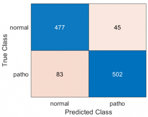
To assess the model's robustness and identify the limitations of its decision boundaries and areas for future improvement, a focused error analysis was conducted on the samples that were incorrectly classified during the cross-validation process. FN, which represent pathological samples the system failed to detect, constitute the primary challenge for detailed analysis in this section. Figure 2 presents the Confusion Matrix (summarizing the overall system performance for voice pathology detection), which outlines the classification results on the unified validation dataset.
Figure 2. Confusion matrix for voice pathology detection
It is observed from the matrix that 83 samples were incorrectly classified as normal (FN), while 45 normal samples were incorrectly classified as pathological (FP). Although the number of FN errors (83) is higher than the number of FP errors (45), indicating a system bias towards specificity, our subsequent analysis will primarily focus on the FN errors. This focus is maintained because the risk of missing a diagnosis (FN) is clinically considered far more critical than the risk of over-referral (FP). Table 10 (Analysis of FN Error Rates and Sample Distribution by Gender) provides the statistical basis for this analysis, offering a detailed breakdown of the FN errors across 15 pathological classifications, specifying the relative contribution of each gender to the overall error rate.
The model demonstrates robust performance and high confidence in detecting pathologies characterized by strong, clear acoustic signatures, resulting in an Overall FN Rate of ≤10% for ten out of fifteen subcategories. This success is primarily driven by the ability to isolate radical acoustic deviations from the normal vocal range.
Table 10. Analysis of false negative error rates and sample distribution by gender (15 pathologies)
|
Pathology |
Total Male Samples |
Male (FN) |
Male FN Rate (%) |
Total Female Samples |
Female (FN) |
Female FN Rate (%) |
Overall FN Rate (%) |
|
Dysodia |
12 |
7 |
58.33 |
10 |
3 |
30.00 |
45.45 |
|
Functional Dysphonia |
23 |
6 |
26.09 |
17 |
5 |
29.41 |
27.50 |
|
Contact Pachydermia |
41 |
7 |
17.07 |
1 |
1 |
100.00 |
19.05 |
|
Hyperfunctional Dysphonia |
25 |
2 |
8.00 |
60 |
15 |
25.00 |
20.00 |
|
Psychogenic Dysphonia |
13 |
4 |
30.77 |
21 |
3 |
14.29 |
20.59 |
|
Laryngitis |
52 |
4 |
7.69 |
27 |
5 |
18.52 |
11.39 |
|
Presbyphonia (Vox Senilis) |
11 |
0 |
0.00 |
14 |
3 |
21.43 |
12.00 |
|
Dysphonia |
28 |
4 |
14.29 |
20 |
0 |
0.00 |
8.33 |
|
Reinke's Edema |
7 |
2 |
28.57 |
43 |
1 |
2.33 |
6.00 |
|
Leukoplakia |
27 |
1 |
3.70 |
6 |
2 |
33.33 |
8.82 |
|
Recurrent laryngeal nerve (RLN) |
53 |
5 |
9.43 |
75 |
8 |
10.67 |
10.16 |
|
Spasmodic Dysphonia |
20 |
2 |
10.00 |
18 |
1 |
5.56 |
7.89 |
|
Vocal Fold Carcinoma |
19 |
1 |
5.26 |
1 |
0 |
0.00 |
5.00 |
|
Vocal Fold Polyp |
22 |
3 |
13.64 |
11 |
0 |
0.00 |
9.09 |
|
Central Laryngeal Movement Disorder (CLMD) |
7 |
0 |
0.00 |
1 |
0 |
0.00 |
0.00 |
|
Total |
360 |
88 |
24.44 |
325 |
47 |
14.46 |
19.71 |
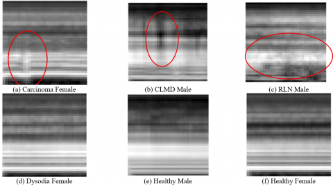
Figure 3. Visual comparison of Gammatone Spectrograms for pathological cases (a, b, c, d) versus healthy samples (e, f). Circles highlight key regions of the pathological acoustic signature in each case: severe noise and harmonic loss in (a) Carcinoma, rapid F0 modulations in (b) Central Laryngeal Movement Disorder (CLMD), broadband noise from air escape in (c) Recurrent laryngeal nerve (RLN) Palsy, and subtle instability in (d) Dysodia
(1) Exceptional Clarity and Detection of Mass Lesions (FN Rate ≤10%): The highest performance is achieved in conditions that induce severe structural or stiffness deviations. This includes Vocal Fold Carcinoma (5%)-where the mass lesion causes severe stiffness, leading to a severe failure in the periodicity of vibration (Figure 3(a)) and Central Laryngeal Movement Disorder (CLMD) (0%), where the severe neurological signature lies outside the normal vocal range (Figure 3(b)). Importantly, while Vocal Fold Polyp (9.09%) is also a mass lesion, its slightly higher FN rate (compared to Carcinoma) suggests that the model is highly sensitive to the stiffness component of the lesion. Polyps, being more compliant (less stiff) than carcinoma, present a moderate challenge. Reinke's Edema (6%) and Leukoplakia (8.82%) also fall into this high-confidence category due to the visible mass/thickness of the vocal folds.
(2) High Confidence in Dynamic Signatures: Excellent performance is also noted for dynamic, prominent signatures. The low FN rate for Recurrent Laryngeal Nerve (RLN) (10.16%) is attributed to Glottal Incompetence, resulting in air escape that the model detects as a broad, broadband noise pattern (Figure 3(c)). Spasmodic Dysphonia (7.89%) and Dysphonia (8.33%) also show high detection rates due to the distinctive acoustic breaks and overall voice disturbance.
(3) Acceptable Performance: Laryngitis (11.39%) and Presbyphonia (Vox Senilis) (12%) demonstrate acceptable performance, with their FN rates slightly exceeding the 10% threshold but remaining within the highly detectable range. This suggests the model successfully captures the acoustic markers associated with generalized inflammation (Laryngitis) and age-related vocal atrophy (Presbyphonia).
4.7.2 Limitations: Ambiguity and functional overlap
The primary vulnerability of the system lies in classifying conditions that either have ambiguous, functional, or overlapping acoustic signatures, leading to a significantly higher FN rate (ranging from 19.05% to 45.45%).
(1) F0 Discrimination Failure in Functional Disorders: The highest error rates are consistently found in functional and soft-acoustic disorders. Dysodia (45.45%) represents the most significant failure. This is due to the subtle pitch change (F0) characterizing Dysodia falling within the wide natural range of healthy vocal variation, preventing the model from setting an accurate decision boundary (Figure 3(d) compared to the healthy control (e) and (f)). Functional Dysphonia (27.50%) and Psychogenic Dysphonia (20.59%) also belong to this group due to the highly variable and effort-driven nature of their vocal signatures, causing significant overlap with normal voice production.
(2) Acoustic Overlap in Tension (Hyperfunctional Dysphonia): The high FN rate for Hyperfunctional Dysphonia (20%) suggests the model confuses the high harmonic energy resulting from pathological hyper-adduction with the high harmonic energy generated by normal vocal effort. This confusion is particularly acute with the Female FN Rate 25%.
4.7.3 Gammatone dependency limits
This analysis confirms that the model relies fundamentally on spectral characteristics reflecting acute and specific physiological lesions (mass or gap), and fails where high accuracy is required to differentiate subtle changes in F0 or minor noise energy from the acoustic characteristics of the normal voice [1].
4.8 Computational efficiency for clinical deployment
To meet the requirements of clinical application demanding high efficiency and maximum inference speed, the system relies on the lightweight SqueezeNet architecture. The model's performance was measured on a standard CPU environment (Intel(R) Core (TM) i5-4300M CPU @ 2.60 GHz with RAM 12.0 GB). To ensure statistical reliability, the inference time was accurately calculated using MATLAB based on the average of 1000 iterations. The measurements resulted in a rapid inference time of 2.06±0.0035 ms for classifying one voice sample. This superior speed confirms that the system is perfectly suited for integration into clinical pre-screening protocols and meets the requirements for real-time or near real-time deployment.
4.9 Performance comparison with others
This comparative analysis aims to evaluate the performance of our proposed system against previous studies in the field of voice pathology detection, with a focus on research that utilized the SVD. This database is considered a fundamental benchmark for system evaluation, and the comparison aims to highlight the effectiveness of our innovative approach in data processing and classification.
Methodological Justification for Comparison: We acknowledge the inherent limitations of cross-study comparisons in our field due to the absence of a unified benchmark, leading to heterogeneity in dataset sizes, pathology types, and evaluation protocols. The primary purpose of Table 11 is not to claim absolute superiority, but rather to contextualize our performance within the broader research landscape and demonstrate that our methodology is highly competitive against recent state-of-the-art approaches. The true reliability of our system is anchored in the rigorous internal validation supported by the 5-Fold Cross-Validation protocol and the reporting of the Mean± Standard Deviation (SD).
The comparative analysis in Table 11 demonstrates that our proposed system achieves a superior performance over previous research, thanks to its strategy of parameter optimization and the use of an efficient neural network. With an overall accuracy of 92.38% (achieved using the Fixed Split Subject-Mixed protocol), our work surpasses all other methods listed. However, it is crucial to note that the final operating point for the system based on the robust 5-Fold CV (Subject-Mixed) protocol achieved an overall accuracy of 88.68 ± 1.25% (F1 Score) and 88.44 ± 1.17% (Accuracy). This final configuration (Configuration 1) was intentionally selected to ensure maximal statistical stability and minimal variance (±1.25% is for F1-score) across all performance metrics, prioritizing robust generalization over the potentially unstable highest recorded accuracy. This confirms that our systematic selection of the optimal parameters for generating Gammatone spectrograms has significantly enhanced the model's ability to detect voice pathologies.
While many previous studies have yielded good results, our system outperforms them. A focused comparison with the highest reported accuracies using the Subject-Mixed protocol highlights our superiority: we significantly outperform the recorded accuracy of 85.77% achieved by Verde et al. [17] (using SVMs and traditional features) and 85.71% achieved by Latiff et al. [22]. Furthermore, our system surpasses complex, state-of-the-art approaches like that of Atmaja and Sasou [36], who utilized an XGBoost Ensemble with advanced SSL features (wav2vec 2.0, HuBERT), yet only achieved an F1 Score of 87.39%. While studies such as Vavrek et al. [35] and Wu et al. [23, 24] achieved accuracies ranging between 71% and 82%, our use of Gammatone spectrograms in conjunction with the SqueezeNet CNN classifier has led to a substantial improvement in performance.
This superiority can be attributed to two key factors:
(1) Innovative Methodology: We employed a sequential optimization study to determine the optimal parameters for the spectrograms, allowing the model to be trained on information-rich and less noisy data.
(2) Classifier Efficiency: The SqueezeNet CNN was chosen for its compact size and high efficiency, ensuring robust performance without requiring a massive number of parameters.
Table 11. Comparison of the proposed system vs. previous works
|
Study |
Healthy Samples |
Pathological Samples & Diagnosis |
Vocal Tasks |
Feature Domains |
Classifier |
Statistical Validation |
Acc% |
|
Verde et al. [17] |
685 |
685 (All types of pathology) |
/a/ |
F0, Jitter, Shimmer, HNR, MFCC |
SVM |
10-Fold CV |
85.77 |
|
Won and Kim [25] |
869Augmented by using MUSAN and MIT IR Survey |
520 (105 Laryngitis, 41 Leukoplakia, 63 Edema, 205 Paralysis, 62 SD, 44 Polyp) (Augmented using MUSAN and MIT IR Survey) |
/a/ |
Mel Spectrogram |
CNN Few-shot Transfer Learning (Pretrained ResNet-18) |
Few-Shot Meta-Testing |
73.7 |
|
Al-Dhief et al. [18] |
687 |
1354 (71 Pathologies) |
/a/, /i/, /u/ |
MFCCs |
OSELM |
Fixed Split |
81.48% |
|
Wu et al. [23, 24] |
482 |
482 (140 Laryngitis, 41 Leukoplakia, 68 Reinke's Edema, 213 RLNP, 22 Carcinoma, 45 Polyps) |
/a/ |
spectrograms |
CNN CNN-CDBN |
Fixed Split |
77 |
|
Ding et al. [26] |
595 |
1090 |
/a/ |
MFSC |
CNN (DCA ResNet) |
Fixed Split |
81.6 |
|
Vavrek et al. [35] |
506 |
506 Organic Dysphonia (Laryngitis, Leukoplakia, Reinke's Edema, Carcinoma, VFP) |
/a/, /i/, /u/ |
spectrograms |
CNN VGG16 |
Fixed Split |
82 |
|
Yagnavajjula et al. [27] |
60 |
60 SD, 60 RLNP |
/a/, /i/, /u/, Sentence |
(WST)-based Features |
feed-forward NN |
10-Fold CV |
82.58 ± 3.02 78.64 ± 3.55 |
|
Tirronen et al. [14] |
587 |
231 (146 Hyperfunctional Dysphonia, 85 VFP) |
/a/ |
wav2vec 2.0 |
SVM |
5-Fold CV |
M. 75.65 F. 74.50 |
|
Javanmardi et al. [11] |
357 |
357 |
/a/ |
Mel Spectrogram |
2D CNN + specAugmenter |
4-Fold CV |
73,4 |
|
Zhou et al. [7] |
687 |
207 structural disease, and 287 neuromuscular disease |
/a/ /i/ and/u/ |
Gammatone Spectral Latitude (GTSL), |
MLP, SVM and RF |
10-Fold CV |
89.9 |
|
Latiff et al. [22] |
140 (SVD), 130 (MVPD |
140 (SVD: various types), 130 (MVPD: unspecified types) |
/a/ |
Mel-Frequency Cepstral Coefficients (MFCC |
OSELM, SVM, DT, NB |
Fixed Split |
85.71 |
|
Atmaja and Sasou [36] |
687 |
1345 (Organic and non-organic voice disorders) |
/a/, /i/, /u/, /aiu/ |
Handcrafted: open SMILE, Praat SSL: wav2vec 2.0, HuBERT, WavLM |
XGBoost Ensemble |
Fixed Split |
F1 Score 87.39 |
|
Ours |
522 |
585 |
/a/ |
Grayscale Gammatone Spectrograms |
CNN SqueezeNet |
Fixed Split
5-Fold CV |
92.38
88.44 ± 1.17 |
Overall, this analysis confirms that the combination of a refined visual representation of acoustic features and the selection of a powerful and efficient classifier has allowed our system to achieve the best overall performance, making it a promising solution for clinical applications.
This study presents a comprehensive methodological framework for identifying the optimal Gammatone spectrogram configuration for vocal fold pathology detection using the SqueezeNet model. This framework has enabled us to determine the optimal combination comprising a frequency range of 80-25000 Hz, a window length of 50 ms, an overlap ratio of 75%, and 41 ERB scale-based filters with grayscale representation.
Although the sequential methodology employed may not guarantee absolute optimality due to parameter interactions, it provided a practical solution balancing accuracy and computational efficiency. To enhance the credibility of the results, we conducted six additional experiments testing configurations near the optimal values, confirming the robustness of performance and reliability of the proposed configuration.
The proposed system achieved remarkable competitive performance, with an accuracy of 92.38% under fixed data split conditions and 88.44 ± 1.17% under five-fold cross-validation, the system demonstrated clinical efficiency due to the selection of the lightweight SqueezeNet classifier, achieving an ultra-fast Inference Time of 2.06 ms, making it highly suitable for real-time preliminary screening applications in clinical settings.
Based on the results and observed methodological challenges, this study opens up promising research avenues:
(1) Gender-Specific Optimization and Separate Modeling: The detailed performance analysis revealed a notable variation between male and female performance, suggesting that unified diagnostic models may be suboptimal. Given the fundamental physiological differences in vocal fold structure, we strongly recommend that future studies adopt a gender-separated parameter optimization methodology from the outset. This approach aims to build two parallel classification systems (one for males and one for females), allowing parameters (e.g., frequency range, number of ERB filters) to be precisely tuned to the unique acoustic characteristics of each physiological group, thereby maximizing overall accuracy and reliability.
(2) Clinical Robustness and Noise Resistance: Clinical deployment necessitates validating the system's robustness against real-world challenges such as variability in recording equipment and background noise interference. Specific simulation experiments should be conducted, including the addition of various types of clinical and environmental noise, to test the system's ability to maintain its performance in non-ideal environments.
(3) Addressing Functional Disorders: The model should be enhanced in the future to better address complex functional disorders that may lack clear acoustic signatures in the spectrogram. This could involve integrating additional acoustic features sensitive to muscle tension or articulatory dynamics.
(4) Exploring Advanced Optimization Techniques: Future studies can leverage more sophisticated global optimization techniques, such as Bayesian Optimization or Genetic Algorithms, to more effectively evaluate parameter interactions and avoid potential local optimization traps.
This work confirms that the integration of refined visual representation of acoustic features with efficient, lightweight deep learning classifiers represents a fertile field for research and development, emphasizing the need for standardized benchmarks and precise statistical evaluations to ensure the successful deployment of these systems in practical clinical applications.
Princess Nourah bint Abdulrahman University Researchers Supporting Project number (PNURSP2025R754), Princess Nourah bint Abdulrahman University, Riyadh, Saudi Arabia.
[1] am Zehnhoff-Dinnesen, A., Neumann, K., Wiskirska-Woźnica, B., Nawka, T. (2020). Phoniatrics I. Springer. https://doi.org/10.1007/978-3-662-46780-0
[2] Maskeliūnas, R., Kulikajevas, A., Damaševičius, R., Pribuišis, K., Ulozaitė-Stanienė, N., Uloza, V. (2022). Lightweight deep learning model for assessment of substitution voicing and speech after laryngeal carcinoma surgery. Cancers, 14(10): 2366. https://doi.org/10.3390/cancers14102366
[3] Morrison, M., Rammage, L., Nichol, H., Pullan, B., May, P., Salkeld, L. (1994). Anatomy and physiology of voice production. The Management of Voice Disorders, pp. 161-200. https://doi.org/10.1007/978-1-4899-2903-7_10
[4] Chaurasiya, H. (2020). Time-frequency representations: Spectrogram, cochleogram and correlogram. Procedia Computer Science, 167: 1901-1910. https://doi.org/10.1016/j.procs.2020.03.209
[5] Sivapatham, S., Kar, A., Christensen, M.G. (2022). Gammatone filter bank-deep neural network-based monaural speech enhancement for unseen conditions. Applied Acoustics, 194: 108784. https://doi.org/10.1016/j.apacoust.2022.108784
[6] Arias-Vergara, T., Klumpp, P., Vasquez-Correa, J.C., Nöth, E., Orozco-Arroyave, J.R., Schuster, M. (2021). Multi-channel spectrograms for speech processing applications using deep learning methods. Pattern Analysis and Applications, 24(2): 423-431. https://doi.org/10.1007/s10044-020-00921-5
[7] Zhou, C., Wu, Y., Fan, Z., Zhang, X., Wu, D., Tao, Z. (2022). Gammatone spectral latitude features extraction for pathological voice detection and classification. Applied Acoustics, 185: 108417. https://doi.org/10.1016/j.apacoust.2021.108417
[8] Islam, R., Abdel-Raheem, E., Tarique, M. (2024). Cochleagram to recognize dysphonia: Auditory perceptual analysis for health informatics. IEEE Access, 12: 59198-59210. https://doi.org/10.1109/ACCESS.2024.3392808
[9] Iandola, F.N., Han, S., Moskewicz, M.W., Ashraf, K., Dally, W.J., Keutzer, K. (2016). SqueezeNet: AlexNet-level accuracy with 50x fewer parameters and< 0.5 MB model size. arXiv preprint arXiv:1602.07360. https://doi.org/10.48550/arXiv.1602.07360
[10] Abdulmajeed, N.Q., Al-Khateeb, B., Mohammed, M.A. (2022). A review on voice pathology: Taxonomy, diagnosis, medical procedures and detection techniques, open challenges, limitations, and recommendations for future directions. Journal of Intelligent Systems, 31(1): 855-875. https://doi.org/10.1515/jisys-2022-0058
[11] Javanmardi, F., Kadiri, S.R., Alku, P. (2024). A comparison of data augmentation methods in voice pathology detection. Computer Speech & Language, 83: 101552. https://doi.org/10.1016/j.csl.2023.101552
[12] Ankışhan, H., İnam, S.Ç. (2021). Voice pathology detection by using the deep network architecture. Applied Soft Computing, 106: 107310. https://doi.org/10.1016/j.asoc.2021.107310
[13] Li, G., Hou, Q., Zhang, C., Jiang, Z., Gong, S. (2021). Acoustic parameters for the evaluation of voice quality in patients with voice disorders. Annals of Palliative Medicine, 10(1): 13036-13136. https://doi.org/10.21037/apm-20-2102
[14] Tirronen, S., Kadiri, S.R., Alku, P. (2023). Hierarchical multi-class classification of voice disorders using self-supervised models and glottal features. IEEE Open Journal of Signal Processing, 4: 80-88. https://doi.org/10.1109/OJSP.2023.3242862
[15] Souissi, N., Cherif, A. (2016). Speech recognition system based on short-term cepstral parameters, feature reduction method and artificial neural networks. In 2016 2nd International Conference on Advanced Technologies for Signal and Image Processing (ATSIP), Monastir, Tunisia, pp. 667-671. https://doi.org/10.1109/ATSIP.2016.7523163
[16] Guo, C., Chen, F., Chang, Y., Yan, J. (2022). Applying random forest classification to diagnose autism using acoustical voice-quality parameters during lexical tone production. Biomedical Signal Processing and Control, 77: 103811. https://doi.org/10.1016/j.bspc.2022.103811
[17] Verde, L., De Pietro, G., Sannino, G. (2018). Voice disorder identification by using machine learning techniques. IEEE Access, 6: 16246-16255. https://doi.org/10.1109/ACCESS.2018.2816338
[18] Al-Dhief, F.T., Latiff, N.M.A., Malik, N.N.N.A., Baki, M.M., Sabri, N., Albadr, M.A.A. (2022). Dysphonia detection based on voice signals using naive bayes classifier. In 2022 IEEE 6th International Symposium on Telecommunication Technologies (ISTT), Johor Bahru, Malaysia, pp. 56-61. https://doi.org/10.1109/ISTT56288.2022.9966535
[19] Kwon, I., Wang, S.G., Shin, S.C., Cheon, Y.I., Lee, B.J., Lee, J.C., Shin, B.J. (2025). Diagnosis of early glottic cancer using laryngeal image and voice based on ensemble learning of convolutional neural network classifiers. Journal of Voice, 39(1): 245-257. https://doi.org/10.1016/j.jvoice.2022.07.007
[20] Abd El Aal, H.A., Taie, S.A., El-Bendary, N. (2021). An optimized RNN-LSTM approach for parkinson’s disease early detection using speech features. Bulletin of Electrical Engineering and Informatics, 10(5): 2503-2512. https://doi.org/10.11591/eei.v10i5.3128
[21] Hidaka, S., Lee, Y., Wakamiya, K., Nakagawa, T., Kaburagi, T. (2020). Automatic estimation of pathological voice quality based on recurrent neural network using amplitude and phase spectrogram. In Interspeech, pp. 3880-3884. http://doi.org/10.21437/Interspeech.2020-3228
[22] Latiff, N.M.A.A., Al-Dhief, F.T., Sazihan, N.F.S.M., Baki, M.M., Malik, N.N.N.A., Albadr, M.A.A., Abbas, A.H. (2025). Voice pathology detection using machine learning algorithms based on different voice databases. Results in Engineering, 25: 103937. https://doi.org/10.1016/j.rineng.2025.103937
[23] Wu, H., Soraghan, J., Lowit, A., Di Caterina, G. (2018). Convolutional neural networks for pathological voice detection. In 2018 40th Annual International Conference of the IEEE Engineering in Medicine and Biology Society (EMBC), Honolulu, USA, pp. 1-4. https://doi.org/10.1109/EMBC.2018.8513222
[24] Wu, H., Soraghan, J., Lowit, A., Di-Caterina, G. (2018) A deep learning method for pathological voice detection using convolutional deep belief networks. Proceedings Interspeech 2018, 446-450. https://doi.org/10.21437/Interspeech.2018-1351
[25] Won, J.H., Kim, D.H. (2024). Metric-based few-shot transfer learning approach for voice pathology detection. IEEE Access, 12: 159226-159238. https://doi.org/10.1109/access.2024.3480523
[26] Ding, H., Gu, Z., Dai, P., Zhou, Z., Wang, L., Wu, X. (2021). Deep connected attention (DCA) ResNet for robust voice pathology detection and classification. Biomedical Signal Processing and Control, 70: 102973. https://doi.org/10.1016/j.bspc.2021.102973
[27] Yagnavajjula, M.K., Mittapalle, K.R., Alku, P., Mitra, P. (2024). Automatic classification of neurological voice disorders using wavelet scattering features. Speech Communication, 157: 103040. https://doi.org/10.1016/j.specom.2024.103040
[28] Patel, R.R., Awan, S.N., Barkmeier-Kraemer, J., Courey, M., Deliyski, D., Eadie, T., Hillman, R. (2018). Recommended protocols for instrumental assessment of voice: American speech-language-hearing association expert panel to develop a protocol for instrumental assessment of vocal function. American journal of Speech-Language Pathology, 27(3): 887-905. https://doi.org/10.1044/2018_AJSLP-17-0009
[29] Adjila, A., Ahfir, M., Ziadi, D. (2021). Silence detection and removal method based on the continuous average energy of speech signal. In 2021 International Conference on Information Systems and Advanced Technologies (ICISAT), Tebessa, Algeria, pp. 1-5. https://doi.org/10.1109/ICISAT54145.2021.9678476
[30] Ma, N., Zhang, X., Zheng, H.T., Sun, J. (2018). ShuffleNet V2: Practical guidelines for efficient CNN architecture design. In European Conference on Computer Vision, pp. 122-138. https://doi.org/10.1007/978-3-030-01264-9_8
[31] Li, D., Cao, W., Hu, Y., Qian, M., Chen, Y., Wei, X. (2025). Lightweight CNN-based algorithm for weld defect recognition. Engineering Research Express, 7(4): 045276. https://doi.org/10.1088/2631-8695/ae1081
[32] He, K., Zhang, X., Ren, S., Sun, J. (2016). Deep residual learning for image recognition. In Proceedings of the IEEE Conference on Computer Vision and Pattern Recognition, pp. 770-778. https://openaccess.thecvf.com/content_cvpr_2016/papers/He_Deep_Residual_Learning_CVPR_2016_paper.pdf.
[33] Simonyan, K., Zisserman, A. (2014). Very deep convolutional networks for large-scale image recognition. arXiv preprint arXiv:1409.1556. https://doi.org/10.48550/arXiv.1409.1556
[34] Tan, M., Le, Q. (2019). EfficientNet: Rethinking model scaling for convolutional neural networks. In International Conference on Machine Learning, pp. 6105-6114. https://doi.org/10.48550/arXiv.1905.11946
[35] Vavrek, L., Hires, M., Kumar, D., Drotár, P. (2021). Deep convolutional neural network for detection of pathological speech. In 2021 IEEE 19th World Symposium on Applied Machine Intelligence and Informatics (SAMI), Herl'any, Slovakia, pp. 000245-000250. https://doi.org/10.1109/SAMI50585.2021.9378656
[36] Atmaja, B.T., Sasou, A. (2025). Pathological voice detection from sustained vowels: Handcrafted vs. self-supervised Learning. In 2025 IEEE International Conference on Acoustics, Speech, and Signal Processing Workshops (ICASSPW), Hyderabad, India, pp. 1-5. https://doi.org/10.1109/ICASSPW65056.2025.11011272