Yong Shi*![]() | Hao Zhang
| Hao Zhang![]()
© 2026 The authors. This article is published by IIETA and is licensed under the CC BY 4.0 license (http://creativecommons.org/licenses/by/4.0/).
OPEN ACCESS
Hyperspectral Image (HSI) classification is a pivotal task in remote sensing. Patch-based methods aim to integrate spatial and spectral information for accurate classification of the central pixel. However, the inherent high dimensionality of HSI data and complex spectral-spatial correlations often lead to substantial parameter counts and high computational costs in existing models. To address these challenges, this paper proposes a novel Lightweight Central pixel-guided Coordinate Attention Network (Lite-C2ANet). The framework introduces three key innovations: First, a Spectral Group Reduction and Interaction (SGRI) module is designed to group adjacent bands and facilitate inter-group information exchange. This effectively reduces spectral redundancy and enables efficient encoding of high-dimensional spectral data. Second, a Central pixel-guided Coordinate Attention (CPCA) module is developed to capture long-range spatial dependencies. It separately aggregates features along horizontal and vertical directions using lightweight shared convolutions, explicitly incorporating spatial coordinate information. Finally, within the CPCA, an Adaptive Central Similarity Guidance (ACSG) mechanism is proposed with negligible parameter overhead. This mechanism adaptively fuses spatial similarity metrics centered on the pivotal central pixel of the patch, guiding the model to focus on the most classification-relevant contextual regions and enhancing the spatial discriminability of class-related attention. Extensive experiments on three public HSI benchmark datasets demonstrate that Lite-C2ANet achieves highly competitive classification accuracy. Crucially, these results are attained with significantly fewer parameters and lower computational overhead compared to state-of-the-art methods, underscoring the effectiveness and efficiency of the proposed lightweight design.
Hyperspectral Image (HSI) classification, lightweight network, Spectral Group Reduction and Interaction, coordinate attention, central pixel guidance
Hyperspectral images (HSIs) can cover a larger spectral range and are widely used to detect visually indistinguishable substances [1-5]. HSIs have extensive applications in precision agriculture, environmental monitoring, urban planning, military reconnaissance, and other fields. HSI classification benefits from rich spectral and spatial information, constituting fundamental research in the field of remote sensing. It can precisely identify ground objects pixel by pixel and detect substances [6-8].
Deep learning has superseded traditional machine learning as the mainstream approach for HSI classification [9]. Meanwhile, the main implementation approach of deep learning methods is to comprehensively combine the spatial-spectral information of the input patch and assign a specific category to the central pixel of the patch [10]. Convolutional neural networks (CNNs), Transformer [11], and more recently Mamba [12] have demonstrated remarkable success in this patch-based classification paradigm. Effective spectral feature extraction is regarded as the critical factor that this paradigm primarily considers, as rich spectral information is crucial for distinguishing different materials with similar textures. Hong et al. [13] extracted local spectral details by generating grouped spectral embeddings in adjacent spectral bands. Similarly, Mei et al. [14] extracted discriminative spatial–spectral features from nonoverlapping subchannels. He et al. [15] performed spectral information in the form of adjacent-interval groups and extracted spatial multidirectional features through hierarchical structures. However, these methods typically process all spectral bands uniformly without considering the varying importance and inter-band correlations, leading to computational redundancy and suboptimal feature representation.
The spatial context reduces the spectral variability within the same class (e.g., the "same object with different spectra" phenomenon) [16]. Consequently, how to effectively capture the spatial distribution relationship of features is another factor that needs to be considered. Wang et al. [17] proposed the contour-adaptive homogeneous region scheme and used Transformer to capture the spatial relationships between regions. Li et al. [18] introduced learnable refocusing parameters to dynamically adjust the key spatial features. Zhang et al. [19] added multiscale and coordinate information in the spatial patch to effectively highlight useful information and weaken useless information. Notably, the ultimate goal of patch-based classification is to accurately assign a label to the central pixel [15]. Undeniably, this central pixel should be the primary focus, as it holds the most decisive spectral signature for the classification decision. However, the above-mentioned methods, in their pursuit of broader contextual information, adopt a holistic approach to feature extraction from the entire patch. This isotropic treatment can inadvertently marginalize the influence of the central pixel, leading to suboptimal feature representation where the contribution of the most informative part of the input is weakened. Some methods pay additional attention to the central pixel. Feng et al. [20] designed a multiple stratified random sampling module to generate features at different levels from the central pixel. Zhang et al. [21] proposed the center-scan mechanism to capture correlations between the central pixel and its surrounding pixels. Yu et al. [22] introduced a center-specific perception Transformer to highlight the spatial weight of class-related attention. Then, the central pixel focus of the above methods often relies on additional sampling strategies or incurs a huge computational burden.
While the challenges of spectral redundancy and central pixel marginalization are often discussed separately in the literature, they are intrinsically intertwined in the context of patch-based HSI classification. The high dimensionality of hyperspectral data forces most existing methods to operate on spatial-spectral patches, where computational constraints lead to uniform processing of all spectral bands. This uniform treatment not only introduces redundancy but also dilutes the discriminative contribution of the central pixel, whose spectral signature is the primary determinant of the classification label. Conversely, attempts to emphasize the central pixel—such as through additional sampling strategies or complex attention mechanisms—often further exacerbate the computational burden, creating a trade-off between accuracy and efficiency. Addressing these interconnected challenges therefore requires a unified framework that simultaneously reduces spectral redundancy while explicitly reinforcing the central pixel’s role in the classification decision.
To address these interconnected challenges, we propose Lightweight Central pixel-guided Coordinate Attention Network (Lite-C2ANet), a unified lightweight architecture in which three components are designed to work in concert rather than as independent modules. The core insight is that effective central pixel guidance becomes computationally feasible only after spectral redundancy is reduced, while the reduced spectral representation itself benefits from being spatially refined with explicit focus on the central pixel. Accordingly, our Spectral Group Reduction and Interaction (SGRI) module first compresses the high-dimensional spectral data through intelligent grouping and cross-group interaction, creating a compact yet discriminative spectral representation. Building upon this compact representation, the Central pixel-guided Coordinate Attention (CPCA) module efficiently captures long-range spatial dependencies by explicitly anchoring its computation around the central pixel and incorporating coordinate information—a strategy that would be computationally prohibitive without prior spectral reduction. Finally, the Adaptive Central Similarity Guidance (ACSG) mechanism fuses the central pixel features with the spatially refined representation using an extremely lightweight gating operation (introducing only a single learnable scalar), adaptively emphasizing class-relevant spatial regions while incurring negligible parameter overhead. Together, these three components form an organic whole where spectral reduction enables efficient spatial attention, and spatial attention in turn enhances the discriminability of the compact spectral features.
The main contributions of this work can be summarized as follows:
(1) We propose Lite-C2ANet, a unified lightweight architecture that jointly addresses spectral redundancy and central pixel marginalization—two intrinsically linked challenges in patch-based HSI classification. Unlike existing methods that treat these issues separately, our framework achieves synergy through a carefully orchestrated pipeline where spectral compression enables efficient spatial attention, and spatial attention in turn enhances the discriminability of central pixel features.
(2) We design a SGRI module that reduces spectral dimensionality through intelligent grouping and enables cross-group information exchange, effectively mitigating computational redundancy while preserving discriminative spectral features.
(3) We develop a CPCA module that efficiently captures long-range spatial dependencies by explicitly anchoring attention computation around the central pixel and incorporating coordinate information. This module’s efficiency is enabled by the prior spectral reduction from SGRI, making it computationally feasible without sacrificing accuracy.
(4) We introduce an ACSG mechanism that adaptively fuses central pixel features with global spatial-spectral representations using an extremely lightweight gating operation. This mechanism further reinforces the central pixel’s role in the classification decision while incurring negligible parameter overhead (only one learnable scalar). Extensive experiments on multiple benchmark datasets demonstrate that Lite-C2ANet achieves state-of-the-art performance with significantly reduced computational costs compared to existing methods.
The rest of this paper is structured as follows: Section 2 reviews related work, Section 3 details our methodology, Section 4 presents experimental results and analysis, and Section 5 concludes this study.
2.1 Convolutional neural network-based hyperspectral image classification
CNN has brought substantial paradigms to HSI classification due to its powerful local feature extraction capability. Pan et al. [23] constructed a dual-branch MugNet by applying 1D convolution to investigate spectral information and 2D convolution to extract spatial information. Chen et al. [24] employed several 3D convolutional layers to extract spectral-spatial features. Roy et al. [25] created an enhanced 3D convolutional network called A2S2K by combining spectral attention with residual connections to increase the accuracy. Yang et al. utilized the depth-wise convolution to capture the local spatial–spectral fusion representations. Zhang et al. [26] introduced the spatial-spectral cross-attention module in order to inject global information while extracting local features. Li et al. [27] combined the multiscale regional growth search method to provide multiscale features for CNN. Although CNN-based methods are successful at capturing local spatial patterns, their limited receptive fields and incapacity to describe long-range dependencies without stacking multiple layers limit their usefulness.
2.2 Transformer-based hyperspectral image classification
Transformer-based methods have garnered significant attention in HSI classification for their superior capability in capturing long-range dependencies through the self-attention mechanism. Peng et al. [28] introduced spatial-spectral semantic tokens with different granularities in the Transformer to enhance classification performance. Fang et al. [29] proposed a unique cluster attention mechanism to improve homogenous local details and discriminative long-range features of Transformer. Sun et al. [30] achieved efficient classification by injecting a Gaussian-weighted feature tokenizer into the Transformer encoder. Huang et al. [31] created local and global Transformer branches and fused them through adaptive weights to make up for the deficiency of the Transformer's ability to extract local features. Ding et al. [32] designed the multi-head spectral-spatial depth attention by integrating depth-separable convolution to replace the standard self-attention in the Transformer. Despite their strengths, the high computational complexity of Transformer poses challenges for HSI applications. Moreover, because the self-attention mechanism inherently treats all tokens equally, it can dilute the critical influence of the central pixel, which is a cornerstone of patch-wise HSI classification, which may ultimately hinder classification performance.
2.3 Mamba-based hyperspectral image classification
Building on the global modeling strength of Transformers while aiming to circumvent their computational complexity, recent studies have begun exploring the Mamba model, which leverages a selective state space mechanism for efficient long-range dependency modeling. Li et al. [33] designed a spatial and spectral Mamba block to simultaneously model long-range interactions of the HSI. He et al. [34] proposed a 3D-spectral–spatial selective scanning to adapt the high-dimensional characteristics of HSI. Yang et al. [35] introduced a position mamba block by fusing multi-stage initial features from the ConvNext backbone. Sheng et al. [36] designed dynamic positional embedding for Mamba and combined CNN with Mamba through two parallel branches to alleviate the computational burden. Mamba is often highlighted for its linear computational complexity compared to the quadratic scaling of Transformer's self-attention, presenting a theoretical advantage for large-scale data. In the context of HSI classification, this architecture shows strong potential for modeling long-range spectral dependencies due to its efficient sequence modeling capability. However, the practical deployment of Mamba-based methods faces two main considerations. First, their parameter size tends to be relatively large, which may be a limiting factor in resource-constrained scenarios. Second, like many deep learning approaches, their performance can be sensitive to the availability of annotated training samples—a common challenge in HSI applications where labeled data are often scarce. These characteristics suggest that while Mamba-based methods are well-suited for scenarios with abundant training data and sufficient computational resources, lightweight architectures remain a practical necessity for applications with limited samples and strict efficiency requirements.
3.1 Overview of the Lightweight Central pixel-guided Coordinate Attention Network
In this study, we propose Lite-C2ANet for HSI classification, which presents a lightweight yet powerful framework for HSI classification. The overall architecture of the proposed Lite-C2ANet is illustrated in Figure 1. Our objective is to predict the class label of the central pixel by effectively leveraging both spectral and spatial information while maintaining computational efficiency. Routinely, given an HSI patch $I \in \mathbb{R}^{C \times H \times W}$, where $H \times W$ refers to spatial size and $C$ is the spectral dimension. First, the SGRI module addresses the spectral redundancy by grouping adjacent bands and enabling inter-group communication, thereby obtaining $F_{\text {spe }} \in \mathbb{R}^{D \times H \times W}$. Subsequently, the CPCA module captures long-range spatial dependencies through a lightweight coordinate-aware mechanism combined with multiscale information. Finally, the ACSG mechanism adaptively emphasizes class-relevant contextual information centered around the pivotal central pixel. The entire framework can be formulated as follows:
$F_{\text {spe}}=\operatorname{SGRI}(I)$ (1)
$F_{\text {spa}}=C P C A\left(F_{\text {spe}}\right)$ (2)
$\hat{y}=\operatorname{Classifier}\left(F_{\text {spa}}\right)$ (3)
where, $\hat{y}$ denotes the predicted class label, and each module is meticulously designed to ensure both effectiveness and efficiency.

Figure 1. Illustration of the Spectral Group Reduction and Interaction (SGRI) module
3.2 Spectral Group Reduction and Interaction
High-dimensional spectral data in HSIs often contain significant redundancy due to high correlation between adjacent bands. To address this challenge, we propose the SGRI module as shown in Figure 1, which strategically reduces spectral dimensionality while preserving discriminative information through intelligent grouping and inter-group communication.
1) Group Reduction. Formally, given an input HSI path $I \in \mathbb{R}^{C \times H \times W}$, we specify the adjacent $g_c$ consecutive bands as a group, generating a total of $G=\left\lfloor\frac{C}{g_c}\right\rfloor$ groups. If there is a part that is insufficient for $g_c$, the remaining channels are $R= C \bmod g_c:$
$X=\left\{I_{g_c}^1, I_{g_c}^2, \ldots, I_{g_c}^G, I_{R, \mathbb{I}_{R>0}}^{G+1}\right\}$ (4)
For the G groups, 1×1 group-wise depthwise convolution layer followed by a BN and a ReLU function is applied to achieve highly efficient parallel computing. The channel numbers in each group have been reduced to half of the original (i.e., $g_c / 2$):
$X_1=\operatorname{ReLU}\left(B N\left(\operatorname{GroupConv}_{1 \times 1}\left(\left\{I_{g_c}^1, I_{g_c}^2, \ldots, I_{g_c}^G\right\}\right)\right)\right)$ (5)
Similarly, for the G+1 group, 1×1 convolution layer followed by a BN and a ReLU function is applied, and the number of output channels is also $g_c / 2$:
$X_2=\operatorname{ReLU}\left(\operatorname{BN}\left(\operatorname{Conv}_{1 \times 1}\left(\left\{I_R^{G+1}\right\}\right)\right)\right)$ (6)
Subsequently, $X_1 \in \mathbb{R}^{G \times \frac{g_c}{2} \times H \times W}$ and $X_2 \in \mathbb{R}^{\frac{g_c}{2} \times H \times W}$ are concatenated to obtain the spectrally-reduced feature $X_r \in \mathbb{R}^{D \times H \times W}, D=\left(G+\mathbb{I}_{R>0}\right) \times \frac{g_c}{2}$ and the $3 \times 3$ convolution is used to supplement the initial spatial information:
$X_r=\operatorname{ReLU}\left(\operatorname{BN}\left(\operatorname{Conv}_{3 \times 3}\left(X_r\right)\right)\right)$ (7)
This reduction strategy ensures that spectral information is compressed in a structured manner, preserving discriminative features while eliminating redundancy.
2) Group Interaction. Following the group reduction phase, the SGRI module incorporates a novel group interaction mechanism that facilitates information exchange between spectrally distinct groups. Specifically, we reshape the $X_r$ to emphasize the group structure for obtaining $Q \in \mathbb{R}^{\hat{G} \times \frac{g_c}{2} \times H \times W}$, $\widehat{G}=G+\mathbb{I}_{R>0}$.
Then, we reorganize the arrangement of the $\hat{G}$ grouped spectral information to enable effective cross-group communication. Specifically, we restructure the feature representation by regrouping features across different spectral groups. More precisely, we extract features from the same spectral position across different spectral groups and reorganize them into new functional groups:
$\widehat{Q}^i=\left[Q_0^i, Q_1^i, \ldots, Q_{\hat{G}}^i,\right], i \in\left[1, \frac{g_c}{2}\right]$ (8)
where, $\widehat{Q} \in \mathbb{R}^{\frac{g_c}{2} \times \widehat{G} \times H \times W}$. Then, we perform convolution operations on the features of each new group respectively to further extract spatial features while obtaining cross-group interaction information:
$F_{\text {spe }}=\operatorname{ReLU}\left(\operatorname{BN}\left(\operatorname{Conv}_{3 \times 3}^i\left(\hat{Q}^i\right)\right)\right)$ (9)
Finally, we reshape the $F_{\text {spe }}$ to $D \times H \times W$. The group interaction allows the model to learn complementary spectral relationships across different band groups, enhancing the discriminative power of the extracted features.
In conclusion, the SGRI module significantly reduces computational complexity through spectral group reduction and it maintains discriminative ability through group interaction. These advantages make the SGRI module particularly suitable for resource-constrained HSI classification.
3.3 Central pixel-guided Coordinate Attention
To capture long-range spatial dependencies while maintaining computational efficiency, we introduce the CPCA module as shown in Figure 2. Unlike conventional attention mechanisms that compute global relationships with quadratic complexity, CPCA decomposes the spatial attention into separate horizontal and vertical directions, achieving linear complexity with respect to spatial dimensions.

Figure 2. Structure of the Central pixel-guided Coordinate Attention (CPCA) module and Adaptive Central Similarity Guidance (ACSG)
Given the spectrally-reduced feature $F_{\text {spe }} \in \mathbb{R}^{D \times H \times W}$, we first compute directional average pooling along each spatial axis to acquire spatial coordinate information:
$X_h=\frac{1}{W} \sum_{j=1}^W F_{\text {spe }}(:,:, j)$ (10)
$X_w=\frac{1}{H} \sum_{i=1}^H F_{\text {spe }}(:, i,:)$ (11)
where, $X_h \in \mathbb{R}^{D \times H} \quad$ and $\quad X_w \in \mathbb{R}^{D \times W}$ represent the horizontally and vertically pooled features, respectively. To capture the multiscale spatial distribution and context information, we split the average pooled features of each spatial dimension into four sub-features of different scales. This process is as follows:
$X_h^i=X_h\left[(i-1) \times \frac{D}{4}: i \times \frac{D}{4},:\right]$ (12)
$X_w^i=X_w\left[(i-1) \times \frac{D}{4}: i \times \frac{D}{4},:\right]$ (13)
where, $X_h^i \in \mathbb{R}^{\frac{D}{4} \times H}$ and $X_w^i \in \mathbb{R}^{\frac{D}{4} \times W}$ represent the $i$-th subfeature of each spatial dimension, where $i \in[1,4]$. Then, we respectively applied the depth-wise 1D convolutions to the four sub-features to obtain multiscale information. In addition, to maintain spatial consistency after decoupling the $H$ and $W$ dimensions, we implicitly model the dependency relationship between the two dimensions using lightweight shared convolution. The entire implementation process is defined as follows:
$\hat{X}_h^i=D W \operatorname{Conv1D}\left(X_h^i, K_i\right)$ (14)
$\hat{X}_w^i=D W \operatorname{Conv} 1 D\left(X_w^i, K_i\right)$ (15)
where, $K_i$ denotes the convolution kernel applied to the $i$-th sub-feature, and its value is [1, 3, 5, 7] to capture multiscale information. To obtain spatial coordinate attention containing different semantics, we concatenate different semantic sub-features and generate spatial attention using group normalization and Sigmoid activation functions. The calculation of the output features is as follows:
$A_h=\sigma\left(G N\left(\operatorname{Concat}\left(\hat{X}_h^i\right)\right)\right)$ (16)
$A_w=\sigma\left(G N\left(\operatorname{Concat}\left(\hat{X}_w^i\right)\right)\right)$ (17)
where, $\sigma$ denotes the sigmoid function, GN represents Group Normalization with 4 groups. The final spatial attention map is obtained through outer product combination:
$A_{s p a}=A_h \odot A_w \odot F_{s p e}$ (18)
At this point, the obtained $A_{s p a}$ lacks the guidance of the critical central pixel features, which may lead to the marginalization of the central pixel. To avoid this problem, we adopt the ACSG module to guide $A_{s p a}$ so that the central pixel can efficiently query the spatial semantic information. Specifically, we extracted the central pixel $P_c \in \mathbb{R}^{1 \times D}$ of $F_{\text {spe }}$ and refined its features using Conv1D convolution, as illustrated in Figure 3. Ultimately, we obtained the refined central pixel $\hat{P}_c \in \mathbb{R}^{1 \times D}$ and input it into the ACSG module for further use.

Figure 3. Overall accuracy (%) with different patch sizes on the three datasets
3.4 Adaptive Central Similarity Guidance
Recognizing that the central pixel contains the most critical information for patch-based classification, we propose the parameter-free ACSG mechanism as shown in Figure 2 to adaptively emphasize class-relevant contextual relationships centered around the pivotal central pixel. Let $\hat{P}_c \in \mathbb{R}^{1 \times D}$ represent the central pixel, and $A_{s p a} \in \mathbb{R}^{D \times H \times W}$ denote the feature map from the previous CPCA module. The ACSG mechanism computes two complementary similarity metrics between the central pixel and all spatial positions. First, we calculate the Euclidean distance-based similarity:
$S_{e u c}(i, j)=\frac{1}{1+\left\|A_{s p a}(i, j)-\hat{P}_c\right\|_2+\epsilon}$ (19)
where, $\epsilon$ is a small constant for numerical stability. Second, we compute the cosine similarity to capture angular relationships:
$S_{c o s}(i, j)=\frac{A_{s p a}(i, j) \cdot \hat{P}_c}{\left\|A_{s p a}(i, j)\right\|_2 \cdot\left\|\hat{P}_c\right\|_2}$ (20)
The adaptive fusion of these similarity measures is achieved through a learnable parameter $\lambda$:
$S=\lambda \cdot \operatorname{softmax}\left(S_{e u c}\right)+(1-\lambda) \cdot \operatorname{softmax}\left(S_{c o s}\right)$
where, $\lambda$ is constrained to [0,1] using a sigmoid function, allowing the network to automatically balance the contribution of each similarity metric based on the input characteristics. The final feature refinement is performed through element-wise multiplication with the fused similarity map:
$F_{s p a}=A_{s p a} \otimes S+A_{s p a}$ (21)
The ACSG mechanism is designed to be effectively parameter-free, as it introduces only a single scalar parameter λ for adaptive similarity fusion, while all other components rely solely on mathematical operations applied to existing feature representations. The ACSG explicitly addresses the fundamental challenge in patch-based classification by ensuring that the central pixel, which contains the most critical information for classification decisions.
4.1 Datasets and experimental settings
1) Datasets: In this study, we conduct experiments on three publicly available HSI datasets to fairly demonstrate the effectiveness and efficiency of the proposed method, including Pavia University (PU), WHU-Hi-LongKou (WHU-LK), and Salinas Valley (SV). In addition, Table 1 and Table 2 report the detailed information of each dataset. In addition, we apply the controlled random sampling technique to prevent patch overlap-related information leaking [37]. To prevent potential model overfitting brought on by the small number of training examples, we also use the data augmentation technique [14]. Furthermore, we only use 1% of PU and SV datasets, and 0.25% of the WHU-LK dataset as a training set.
2) Evaluation Metrics: Three common evaluation indicators are employed to quantitatively compare the classification performance of all methods, including Overall Accuracy (OA), Average Accuracy (AA), and Kappa Coefficient (k). To demonstrate the efficiency of the proposed Lite-C2ANet, we additionally apply four evaluation indicators to exploit the computational cost and efficiency of the model, including the Training Time (Train), Inference Time (Infer), Number of Parameters (Params), and Floating Point Operations (FLOPs).
3) Implementation Details: All experiments are conducted on a PC equipped with an Intel(R) Xeon(R) Silver 4310 CPU and an NVIDIA GeForce RTX 3090 24 GB GPU, utilizing PyTorch 2.5.1 and Python 3.10. The epoch and batch size are set to 100 and 64, respectively. The optimizer and learning rate are identical to the most suitable parameters in the study that we compared in order to guarantee the model's optimal performance. We employ the Adam optimizer for the suggested approach, setting $\beta_1$ to 0.9 and $\beta_2$ to 0.999. To keep things simple, the learning rate is set at 0.001.
4) Competitive Approaches: To comprehensively validate the effectiveness of our proposed Lite-C2ANet, three types of representative HSI classification architectures are chosen: CNN-based (A2S2K [25], CSCANet [26]), transformer-based (ELS2T [19], LRDTN [32]), and Mamba-based (IGroupSSMamba [15], MambaHSI [33], 3DSSMamba [34]). We compare the three HSI datasets both quantitatively and qualitatively using the same distribution of training samples while keeping the best settings from the original published code for each approach.
Table 1. Sample numbers of training set, validation set, and test set of each class on Pavia University dataset and WHU-Hi-LongKou dataset
|
No. |
Pavia University |
WHU-Hi-LongKou |
||||||
|
Name |
Training |
Validation |
Test |
Name |
Training |
Validation |
Test |
|
|
1 |
Asphalt |
66 |
66 |
6499 |
Corn |
86 |
86 |
34339 |
|
2 |
Meadows |
186 |
187 |
18276 |
Cotton |
21 |
21 |
8332 |
|
3 |
Gravel |
21 |
21 |
2057 |
Sesame |
7 |
8 |
3016 |
|
4 |
Trees |
30 |
31 |
3003 |
Broad-leaf soybean |
158 |
158 |
62896 |
|
5 |
Metal sheets |
14 |
13 |
1318 |
Narrow-leaf soybean |
11 |
10 |
4130 |
|
6 |
Bare Soil |
50 |
50 |
4929 |
Rice |
30 |
29 |
11795 |
|
7 |
Bitumen |
13 |
14 |
1303 |
Water |
167 |
168 |
66721 |
|
8 |
Bricks |
37 |
37 |
3608 |
Roads and houses |
18 |
18 |
7088 |
|
9 |
Shadows |
10 |
9 |
928 |
Mixed weed |
13 |
13 |
5203 |
|
- |
Total |
427 |
428 |
41921 |
Total |
511 |
511 |
203520 |
Table 2. Sample numbers of training set, validation set, and test set of each class on Salinas Valley dataset
|
No. |
Salinas Valley |
|||
|
Name |
Training |
Validation |
Test |
|
|
1 |
Broccoli green weeds 1 |
20 |
20 |
1969 |
|
2 |
Broccoli green weeds 2 |
37 |
37 |
3652 |
|
3 |
Fallow |
20 |
20 |
1936 |
|
4 |
Fallow rough plow |
14 |
14 |
1366 |
|
5 |
Fallow smooth |
27 |
27 |
2624 |
|
6 |
Stubble |
39 |
40 |
3880 |
|
7 |
Celery |
36 |
36 |
3507 |
|
8 |
Grapes untrained |
113 |
112 |
11046 |
|
9 |
Soil vinyard develop |
62 |
62 |
6079 |
|
10 |
Corn senesced green weeds |
33 |
33 |
3212 |
|
11 |
Lettuce romaine 4wk |
11 |
10 |
1047 |
|
12 |
Lettuce romaine 5wk |
19 |
20 |
1888 |
|
13 |
Lettuce romaine 6wk |
9 |
9 |
898 |
|
14 |
Lettuce romaine 7wk |
10 |
11 |
1049 |
|
15 |
Vinyard untrained |
73 |
72 |
7123 |
|
16 |
Vinyard vertical trellis |
18 |
18 |
1771 |
|
- |
Total |
541 |
541 |
53047 |
4.2 Parameter analysis
1) Different Input Patch Size: The spatial size of the patch affects the amount of spatial neighbor information it includes, which influences the model's performance in patch-based HSI classification. We set H equal to W, and within the range of spatial sizes from $5 \times 5$ to $15 \times 15$, find the optimal spatial sizes for three datasets. Figure 3 presents the corresponding experimental results. It is evident that on PU and WHU-LK, the OA typically exhibits a trend of initially rising and then declining as spatial size increases. The accuracy curve either drops or rises slowly when the spatial dimension exceeds $9 \times 9$. This indicates that as spatial information becomes richer, the classification performance of the model is getting better and better. On the SV datasets, there is a positive correlation between the OA trend and the classification accuracy and patch size. However, when the spatial size is too large, it will lead to overfitting of the model. Taking into account the model performance and computational cost comprehensively, in the following experiment, we set the patch size to $9 \times 9$.

Figure 4. Overall accuracy (%) with different numbers of $g_c$ in Spectral Group Reduction and Interaction (SGRI)
2) Different Numbers of $g_c$ in SGRI: In the proposed Lite-C2ANet, the number of adjacent bands $g_c$ in each group of SGRI should be determined. As shown in Figure 4, we conduct experiments on three datasets with {8, 16, 24, 32, 40}. It is obvious that when the number of adjacent bands $g_c$ selected is relatively small, the input spectral information is too fragmented, resulting in poor model performance. Similarly, when $g_c$ is too large, the increase in spectral-independent information leads to varying degrees of performance degradation on different datasets. When the parameter $g_c$ is set to be 16, our proposed method can obtain the highest classification on PU and SV datasets. On the WHU-LK dataset, the model performs best when $g_c$=24. The possible reason is that this dataset contains more extensive spectral information. Taking into account the generalization of the model on different datasets and its performance comprehensively, we adopt $g_c$=16 in practical applications.
4.3 Classification results and visual evaluation
We perform evaluations on the PU, WHU-LK, and SV datasets. The quantitative results from all approaches on OA, AA, and Kappa metrics are presented in Tables 3-5. To lessen the experiment's contingency and variability, five different tests are carried out to find the average results and standard deviation for each model. Additionally, corresponding visualization maps were produced by choosing the approach with the highest OA for each of the five tests, as shown in Figures 5-7.
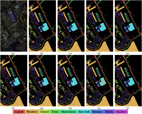
1) The PU dataset: Table 3 and Figure 5 present the classification results and visualization maps of different methods on the PU dataset. As can be shown, the suggested Lite-C2ANet exhibits significant efficacy and superiority when compared to other researched methods. The CNN-based methods include A2S2K and CSCANet, which incorporate attention mechanisms while utilizing local receptive fields, resulting in competitive outcomes. However, compared with the proposed Lite-C2ANet, they still demonstrate a substantial accuracy reduction. Transformer-based and Mamba-based architectures establish long-range dependencies, but there are varying degrees of overfitting when the amount of data is limited. While recent ELS2T and LRDTN approaches incorporate multiscale features into the transformer network, they still fall short of Lite-C2ANet in terms of performance. Comparatively, Lite-C2ANet performs global contextual modeling with central pixel guidance with spectral group information. The coordinate attention in CPCA can efficiently capture long-distance relationships of different scales while remaining lightweight. The IGroupSSMamba and MambaHSI combined the group information of the spectrum in different ways, but showed poorer results in categories with less data volume, such as gravel and bitumen. In contrast, the group dimension reduction and interaction strategy of Lite-C2ANet can retain most of the spectral information with fewer parameters. Compared with the 3DSSMamba approach, the quantitative improvements of OA, AA, and Kappa up to 7.62%, 10.5%, and 10.14%, respectively, were observed. The visualization maps of several comparison techniques are shown in Figure 3 to further highlight the variations in categorization outcomes. It is evident that the suggested Lite-C2ANet achieves unambiguous category borders with few artifacts and shows the most consistent findings with the ground truth.
Table 3. Classification results obtained by different methods for Pavia University dataset
|
Class |
Convolutional Neural Network-Based |
Transformer-Based |
Mamba-Based |
Lightweight Central pixel-guided Coordinate Attention Network |
||||
|
Attention-based 2-Stage Spectral-Spatial Kernel |
Convolutional Spatial–Channel Attention Network |
Enhanced Lightweight Spectral-Spatial Transformer |
Low-Rank Deep Tensor Network |
Iterative Group Spectral–Spatial Mamba Network |
Multi-Attention Mamba for Hyperspectral Image |
3D Spectral–Spatial Mamba Network |
||
|
1 |
98.10±1.23 |
98.40±1.01 |
98.51±0.77 |
98.34±0.77 |
97.32±0.72 |
95.26±0.90 |
94.72±0.41 |
97.95±1.32 |
|
2 |
99.46±0.41 |
99.87±0.10 |
99.34±0.46 |
99.45±0.41 |
99.32±0.50 |
98.94±0.55 |
96.14±1.33 |
99.94±0.05 |
|
3 |
90.25±7.02 |
86.81±5.21 |
90.43±3.78 |
91.45±5.49 |
86.67±3.52 |
87.35±4.02 |
67.38±3.76 |
94.34±2.11 |
|
4 |
98.16±0.93 |
98.24±0.20 |
95.29±2.88 |
97.39±0.90 |
97.96±0.47 |
93.38±2.64 |
94.00±4.38 |
97.64±0.52 |
|
5 |
99.98±0.03 |
100.00±0.00 |
99.71±0.50 |
99.71±0.27 |
100.00±0.00 |
100.00±0.00 |
93.99±5.03 |
100.00±0.00 |
|
6 |
99.18±0.72 |
99.12±0.47 |
99.31±0.92 |
98.16±1.34 |
96.46±2.45 |
95.08±1.73 |
79.06±4.46 |
99.45±0.41 |
|
7 |
92.33±5.08 |
95.55±1.14 |
91.08±7.25 |
73.83±37.12 |
93.14±1.56 |
88.21±6.65 |
73.66±6.24 |
98.66±1.92 |
|
8 |
96.98±2.43 |
95.25±2.41 |
94.87±3.03 |
91.92±2.97 |
96.20±1.70 |
97.51±1.24 |
90.10±1.66 |
96.14±1.33 |
|
9 |
99.63±0.25 |
95.11±4.31 |
97.76±1.47 |
98.45±1.27 |
99.29±0.42 |
97.03±2.33 |
99.40±0.41 |
98.84±0.64 |
|
Overall Accuracy (%) |
98.26±0.25 |
98.16±0.26 |
97.81±0.58 |
97.13±1.19 |
97.52±0.44 |
96.48±0.40 |
91.13±0.95 |
98.75±0.17 |
|
Average Accuracy (%) |
97.12±0.65 |
96.48±0.81 |
96.25±1.17 |
94.30±4.07 |
96.26±0.34 |
94.75±0.62 |
87.61±1.66 |
98.11±0.17 |
|
Kappa Coefficient ×100 |
97.69±0.33 |
97.56±0.35 |
97.10±0.77 |
96.18±1.59 |
96.71±0.58 |
95.33±0.54 |
88.20±1.30 |
98.34±0.23 |
Figure 5. Classification maps using different classification methods on the Pavia University (PU) dataset: (a) False-color image, (b) Ground-truth map, (c) Attention-based 2-Stage Spectral-Spatial Kernel (A2S2K), (d) Convolutional Spatial–Channel Attention Network (CSCANet), (e) Enhanced Lightweight Spectral-Spatial Transformer (ELS2T), (f) Low-Rank Deep Tensor Network (LRDTN), (g) Iterative Group Spectral–Spatial Mamba Network (IGroupSSMamba), (h) Multi-Attention Mamba for Hyperspectral Image (MambaHSI), (i) 3D Spectral–Spatial Mamba Network (3DSSMamba), (j) Proposed Lightweight Central pixel-guided Coordinate Attention Network (Lite-C2ANet)
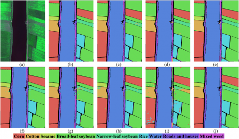
2) The WHU-LK dataset: Table 4 and Figure 6 present the classification results and visualized maps obtained of different methods on the WHU-LK dataset. The results demonstrate that the proposed Lite-C2ANet consistently exceeds other competitive methods by significant margins, exhibiting the largest amounts across all three parameters. Compared to A2S2K and CSCANet, the proposed Lite-C2ANet performs better in OA by 0.57% and 0.39%, respectively, which achieves competitive performance with fewer parameters and higher efficiency. Due to the limitation of sample size, the Transformer-based methods perform poorly in classifying categories such as sesame, soybean, and mixed weed. The AA is reduced by 3.82% and 2.15%, respectively, compared with the proposed method. Thanks to the effective spectral extraction of SGRI and the CPCA module, Lite-C2ANet shows an improvement of 1.12%, 1.17%, and 5.77% in OA and 3.27%, 3.09%, and 22.18% in the Kappa compared to Mamba-based methods. In contrast, the proposed method achieves excellent performance even with a limited sample size due to its lightweight design and efficient feature extraction strategy, with OA, AA, and Kappa values of 99.46%, 98.11%, and 99.29%, respectively. From the qualitative results shown in Figure 6, in comparison with these methods, the Lite-C2ANet obtains clean and more accurate classification results with better object integrity and clearer boundaries.
Table 4. Classification results obtained by different methods for WHU-Hi-LongKou (WHU-LK) dataset
|
Class |
Convolutional Neural Network-Based |
Transformer-Based |
Mamba-Based |
Lightweight Central pixel-guided Coordinate Attention Network |
||||
|
Attention-Based 2-Stage Spectral-Spatial Kernel |
Convolutional Spatial–Channel Attention Network |
Enhanced Lightweight Spectral-Spatial Transformer |
Low-Rank Deep Tensor Network |
Iterative Group Spectral–Spatial Mamba Network |
Multi-Attention Mamba for Hyperspectral Image |
3D Spectral–Spatial Mamba Network |
||
|
1 |
99.83±0.07 |
99.97±0.01 |
99.50±0.56 |
99.89±0.08 |
99.70±0.36 |
99.88±0.11 |
98.09±1.17 |
99.91±0.03 |
|
2 |
98.49±1.22 |
98.76±1.60 |
95.91±2.32 |
98.51±0.79 |
98.90±0.60 |
96.99±2.82 |
88.90±3.96 |
99.64±0.27 |
|
3 |
89.66±4.32 |
89.53±2.22 |
93.36±2.92 |
91.84±3.01 |
91.37±6.89 |
92.25±1.43 |
19.62±12.39 |
97.60±3.09 |
|
4 |
99.29±0.41 |
99.36±0.18 |
98.86±0.49 |
99.45±0.18 |
98.36±0.80 |
98.49±0.99 |
96.63±0.85 |
99.77±0.11 |
|
5 |
91.24±3.59 |
95.87±1.97 |
88.07±5.03 |
91.57±4.01 |
86.05±2.52 |
90.45±4.54 |
33.40±8.92 |
96.52±1.85 |
|
6 |
99.43±0.36 |
99.84±0.07 |
98.10±1.97 |
98.96±0.99 |
98.87±0.79 |
97.86±1.56 |
87.85±7.42 |
99.79±0.10 |
|
7 |
99.96±0.03 |
99.97±0.03 |
99.67±0.53 |
99.84±0.28 |
99.94±0.07 |
99.82±0.24 |
99.94±0.09 |
99.94±0.03 |
|
8 |
94.46±2.76 |
93.90±3.01 |
89.21±4.48 |
90.61±4.15 |
93.19±3.28 |
91.12±4.39 |
81.58±7.46 |
95.37±1.41 |
|
9 |
90.93±3.71 |
92.10±3.62 |
85.97±4.55 |
92.97±3.27 |
87.18±2.37 |
88.33±6.00 |
77.35±9.81 |
94.47±1.27 |
|
Overall Accuracy (%) |
98.89±0.13 |
99.07±0.13 |
98.10±0.42 |
98.84±0.17 |
98.34±0.23 |
98.29±0.42 |
93.69±0.47 |
99.46±0.02 |
|
Average Accuracy (%) |
95.92±0.86 |
96.59±0.49 |
94.29±1.34 |
95.96±0.66 |
94.84±1.05 |
95.02±0.90 |
75.93±1.27 |
98.11±0.30 |
|
Kappa Coefficient ×100 |
98.54±0.17 |
98.78±0.17 |
97.50±0.55 |
98.47±0.22 |
97.82±0.30 |
97.75±0.55 |
91.67±0.63 |
99.29±0.02 |
Figure 6. Classification maps using different classification methods on the WHU-Hi-LongKou (WHU-LK) dataset: (a) False-color image, (b) Ground-truth map, (c) Attention-based 2-Stage Spectral-Spatial Kernel (A2S2K), (d) Convolutional Spatial–Channel Attention Network (CSCANet), (e) Enhanced Lightweight Spectral-Spatial Transformer (ELS2T), (f) Low-Rank Deep Tensor Network (LRDTN), (g) Iterative Group Spectral–Spatial Mamba Network (IGroupSSMamba), (h) Multi-Attention Mamba for Hyperspectral Image (MambaHSI), (i) 3D Spectral–Spatial Mamba Network (3DSSMamba), (j) Proposed Lightweight Central pixel-guided Coordinate Attention Network (Lite-C2ANet)
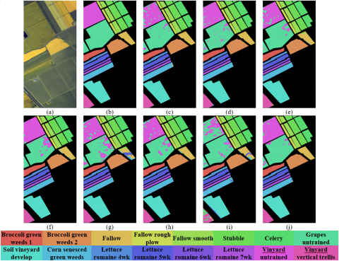
3) The SV dataset: Table 5 and Figure 7 present the classification results and visualized maps obtained by different methods for the SV dataset. The results illustrate that the proposed Lite-C2ANet performs superior in classification when compared to other approaches. In contrast to the CNN-based methods, the OA of Lite-C2ANet is 0.54% higher than A2S2K and 0.08% higher than CSCANet, which illustrates the powerful representation ability of our method. Furthermore, compared to Transformer-based methods, Lite-C2ANet gains about 1.76% and 1.55% improvement in OA, respectively. further revealing the effectiveness of our coordinate attention and central similarity guidance. Compared to Mamba-based methods, Lite-C2ANet demonstrates notable improvements in OA by 4.44%, 1.68%, and 10.68%, respectively, proving the advantages of the proposed model under the condition of limited data volume. In addition, the corresponding classification maps generated by comparison approaches are visualized in Figure 7. The proposed Lite-C2ANet delivers the high-quality classifications and well-maintained boundaries across most regions.
Table 5. Classification results obtained by different methods for Salinas Valley (SV) dataset
|
Class |
Convolutional Neural Network-Based |
Transformer-Based |
Mamba-Based |
Lightweight Central pixel-guided Coordinate Attention Network |
||||
|
Attention-Based 2-Stage Spectral-Spatial Kernel |
Convolutional Spatial–Channel Attention Network |
Enhanced Lightweight Spectral-Spatial Transformer |
Low-Rank Deep Tensor Network |
Iterative Group Spectral–Spatial Mamba Network |
Multi-Attention Mamba for Hyperspectral Image |
3D Spectral–Spatial Mamba Network |
||
|
1 |
98.60±2.22 |
99.90±0.10 |
99.70±0.27 |
99.24±1.47 |
99.74±0.48 |
99.47±0.65 |
91.76±5.22 |
99.89±0.15 |
|
2 |
99.96±0.08 |
99.61±0.18 |
99.76±0.21 |
99.99±0.02 |
99.76±0.30 |
99.99±0.01 |
99.73±0.15 |
100.00±0.00 |
|
3 |
97.20±2.65 |
99.95±0.08 |
95.08±3.44 |
95.61±6.01 |
85.10±18.88 |
95.74±2.96 |
79.97±6.95 |
99.96±0.05 |
|
4 |
99.74±0.23 |
99.21±0.55 |
98.29±1.28 |
99.11±0.44 |
97.82±1.38 |
96.40±3.22 |
98.68±0.63 |
98.52±0.64 |
|
5 |
98.12±0.66 |
98.25±1.07 |
96.17±4.41 |
98.59±1.90 |
97.15±3.08 |
99.05±1.63 |
95.35±2.18 |
98.56±2.14 |
|
6 |
100.00±0.00 |
99.97±0.06 |
99.54±0.46 |
100.00±0.00 |
99.99±0.02 |
99.98±0.04 |
98.82±0.75 |
99.87±0.25 |
|
7 |
99.88±0.17 |
99.94±0.06 |
99.70±0.17 |
99.88±0.19 |
99.50±0.38 |
99.97±0.06 |
98.48±1.06 |
100.00±0.00 |
|
8 |
95.03±2.89 |
94.23±1.98 |
94.79±1.02 |
90.14±2.28 |
86.89±3.78 |
91.23±0.99 |
84.41±3.14 |
93.48±0.60 |
|
9 |
99.88±0.10 |
99.97±0.06 |
99.09±1.05 |
100.00±0.00 |
99.45±0.57 |
99.71±0.35 |
96.36±2.23 |
100.00±0.00 |
|
10 |
96.72±2.11 |
97.93±1.38 |
97.22±1.71 |
95.88±4.09 |
95.41±2.03 |
97.99±1.55 |
85.34±7.90 |
97.23±1.57 |
|
11 |
99.22±0.35 |
97.50±2.15 |
97.36±0.74 |
99.60±0.63 |
96.26±4.13 |
98.05±1.17 |
57.04±10.67 |
99.79±0.27 |
|
12 |
98.87±2.27 |
99.87±0.21 |
99.29±0.87 |
99.97±0.03 |
99.64±0.30 |
99.93±0.12 |
97.83±3.15 |
99.71±0.25 |
|
13 |
97.95±3.24 |
99.18±1.00 |
98.71±1.20 |
98.13±2.55 |
98.02±2.52 |
99.04±1.35 |
97.66±1.53 |
98.51±1.93 |
|
14 |
98.02±1.27 |
98.00±0.35 |
98.00±0.80 |
99.29±0.31 |
98.02±1.64 |
99.37±0.25 |
98.21±1.02 |
98.76±0.81 |
|
15 |
91.90±4.72 |
94.85±2.37 |
86.57±3.85 |
92.04±2.72 |
85.87±4.79 |
89.17±2.04 |
59.82±11.24 |
96.32±1.79 |
|
16 |
98.14±1.62 |
98.31±0.85 |
93.65±4.96 |
97.41±3.85 |
95.29±4.31 |
96.87±3.91 |
80.24±8.29 |
98.95±0.96 |
|
Overall Accuracy (%) |
97.21±0.38 |
97.67±0.34 |
95.99±0.79 |
96.20±0.60 |
93.91±1.16 |
96.07±0.31 |
86.89±1.48 |
97.75±0.21 |
|
Average Accuracy (%) |
98.08±0.40 |
98.54±0.31 |
97.06±0.59 |
97.81±0.66 |
95.87±1.56 |
97.62±0.44 |
88.73±1.55 |
98.72±0.15 |
|
Kappa Coefficient ×100 |
96.89±0.43 |
97.41±0.38 |
95.54±0.88 |
95.77±0.67 |
93.23±1.29 |
95.63±0.35 |
85.36±1.67 |
97.50±0.24 |
Figure 7. Classification maps using different classification methods on the Salinas Valley (SV) dataset: (a) False-color image, (b) Ground-truth map, (c) Attention-based 2-Stage Spectral-Spatial Kernel (A2S2K), (d) Convolutional Spatial–Channel Attention Network (CSCANet), (e) Enhanced Lightweight Spectral-Spatial Transformer (ELS2T), (f) Low-Rank Deep Tensor Network (LRDTN), (g) Iterative Group Spectral–Spatial Mamba Network (IGroupSSMamba), (h) Multi-Attention Mamba for Hyperspectral Image (MambaHSI), (i) 3D Spectral–Spatial Mamba Network (3DSSMamba), (j) Proposed Lightweight Central pixel-guided Coordinate Attention Network (Lite-C2ANet)
4.4 Ablation studies
1) Ablation Study of the Proposed Modules: To evaluate the effectiveness of each module in Lite-C2ANet, including SGRI, CPCA, and ACSG, we conduct ablation experiments on three datasets with the classification metrics and model’s parameters.
Table 6 shows the results of the ablation experiments. In Case 1, to verify the contribution and influence of SGRI, we replaced it with standard convolution. It can be observed that the impact of SGRI on OA is acceptable, but its influence on the number of parameters is extremely important. After being replaced with standard convolution, the number of parameters increased by more than ten times, indicating that SGRI has the ability to efficiently reduce dimensions and preserve information. In Case 2, we use Vision Transformer (ViT) to replace CPCA to verify its importance. However, since ViT is more suitable for natural images, the classification results for HSI are not very satisfactory, which proves the long-distance dependency extraction ability of CPCA. In Case 3, we removed the ASCG module, and the number of parameters in the model remained almost unchanged. It is precisely because of the parameter-free manner of ASCG that the parameter efficiency is improved while providing the importance of the central pixel for the proposed model. In Case 4, our complete Lite-C2ANet offers the best performance and the fewest parameters, demonstrating its effectiveness in resource-constrained situations.
Table 6. Ablation study of the proposed modules
|
Cases |
Spectral–Spatial Gradient Residual Image |
Central pixel-guided Coordinate Attention |
Adaptive Coordinate Spatial Gating |
Convolution |
Vision Transformer |
Pavia University |
WHU-Hi-LongKou |
Salinas Valley |
|||
|
Overall Accuracy (%) |
Parameters |
Overall Accuracy (%) |
Params |
Overall Accuracy (%) |
Parameters |
||||||
|
1 |
× |
√ |
√ |
√ |
× |
98.19 |
66.59 |
99.45 |
377.86 |
97.32 |
223.32 |
|
2 |
√ |
× |
× |
× |
√ |
97.85 |
20.04 |
99.02 |
94.82 |
95.37 |
58.74 |
|
3 |
√ |
√ |
× |
× |
× |
97.98 |
5.85 |
99.15 |
14.71 |
95.86 |
11.13 |
|
4 |
√ |
√ |
√ |
× |
× |
98.75 |
5.85 |
99.46 |
14.71 |
97.75 |
11.13 |
2) Ablation Study of the Percentage of Training Samples: To demonstrate the robustness of the proposed Lite-C2ANet, we perform extensive experiments with comparison methods by varying the proportions of training samples. Specifically, the training sample percentage is set between 0.25% and 1.5%, as shown in Figure 8. Red curves clearly show that the suggested Lite-C2ANet yields the maximum OA for different training sample ratios, further demonstrating the method's superiority and robustness. From the results, the classification accuracy of all methods shows a consistent upward trend as the percentage of training samples rises. When the sample size is small, the proposed method demonstrates significant advantages due to its efficient lightweight design. The advantage gradually diminishes as the sample size grows because of the comparison method's parameter strategy. It is worth noting that 3DSSMamba has always maintained a relatively low classification level. The main reason for this is that its powerful feature extraction capability can lead to overfitting when samples are limited.

(a)

(b)

(c)
Figure 8. Classification performance under different training samples: (a) Pavia University (PU). (b) WHU-Hi-LongKou (WHU-LK). (c) Salinas Valley (SV)
4.5 Complexity analysis
A comprehensive assessment of the complexity of the competitive approaches is carried out in order to assess the computing efficiency of the suggested model. In Table 7, the proposed Lite-C2ANet has the minimum number of parameters and the highest computational efficiency. on the one hand, this is attributed to the fact that SGRI efficiently reduces the spectral dimension and extracts spectral interaction information. On the other hand, CPCA efficiently handles spatial long-range dependencies and applies central pixels for guidance without parameters. Compared with the practice of stacking convolutional layers based on the CNN method, the SGRI module of the proposed model can complete spectral dimensionality reduction in a more efficient and lightweight way and maintain the information extraction ability. For Transformer-based methods, the proposed model's CPCA module achieves CPCA with the fewest parameters to obtain long-distance dependencies. In comparison to the proposed Lite-C2ANet, Mamba is still constrained by the number of parameters and computational load when the sample size of HSI is small, despite having comparatively modest FLOPs. Specifically, the suggested approach outperforms other models in terms of inference time across all datasets. On the PU dataset, the proposed method has only 5.58 K, just about 0.66% of CSCANet, and is still 6 K lower than the ELS2T and 18.29 K lower than the minimal model 3DSSMamba. On the WHU-LK datasets, Lite-C2ANet outperforms the other methods with 14.71 K parameters and 0.89 M FLOPs, respectively, achieving the optimal training and inference times. The following is our specific analysis of SGRI and CPCA:
1) Complexity Analysis of Group Reduction in SGRI: Given an input $I \in \mathbb{R}^{C \times H \times W}$ and a kernel size $K \times K$, the FLOPs for the Group Reduction module is:
$\mathrm{FLOPs}^{\text {SGRI }}=\widehat{G} \times\left(H \times W \times g_c \times \frac{g_c}{2} \times K \times K\right)$ (22)
where, $\widehat{G} \times g_c \approx C$, this can be simplified to approximately $H \times W \times C \times \frac{g_c}{2} \times K \times K$. In contrast, the FLOPs for the standard convolutional layer is:
FLOPs $^{\text {std }}=H \times W \times C \times D \times K \times K$ (23)
The parameter count follows the same trend. The standard convolution requires $C \times D \times K \times K$ parameters. In contrast, the group reduction requires only $C \times \frac{g_c}{2} \times K \times K$ parameters. Given that $D \approx \frac{C}{2}$ and $g_c \ll C$, the proposed Group Reduction module achieves a theoretical reduction in computational complexity and parameter count by a factor of approximately $\frac{g_c}{c}$ compared to a standard convolution layer. This advantage makes group reduction particularly efficient for processing high-dimensional data.
2) Complexity Analysis of CPCA: Given the spectrally-reduced feature $F_{\text {spe }} \in \mathbb{R}^{D \times H \times W}$, and convolution kernel size $K_i$ applied to the $i$-th sub-feature, where $i \in[1,4]$, the FLOPs for the CPCA module is derived as follows:
$\mathrm{FLOPs}^{C P C A}=\sum_{i=1}^4\left(K_i \times H \times \frac{D}{4}+K_i \times W \times \frac{D}{4}\right)$ (24)
Substituting the kernel sizes $K_i$= [1, 3, 5, 7], the FLOPs of CPCA can be expressed as:
$\mathrm{FLOPs}^{C P C A}=4 D(H+W)$ (25)
This linear scaling O(D(H+W)) stands in sharp contrast to the quadratic complexity O(D(HW2)) of standard Transformer self-attention and offers superior parameter efficiency even compared to the linear scaling O(DHW) of selective state-space models like Mamba, making CPCA highly efficient for high-resolution HSI analysis.
Table 7. Comparison of Number of Parameters (Params), Floating Point Operations (FLOPs), Training Time (Train), and Inference Time (Infer) of different models on experimental datasets
|
Datasets |
Efficiency |
Convolutional Neural Network-Based |
Transformer-Based |
Mamba-Based |
Lightweight Central pixel-guided Coordinate Attention Network |
||||
|
Attention-Based 2-Stage Spectral-Spatial Kernel |
Convolutional Spatial–Channel Attention Network |
Enhanced Lightweight Spectral-Spatial Transformer |
Low-Rank Deep Tensor Network |
Iterative Group Spectral–Spatial Mamba Network |
Multi-Attention Mamba for Hyperspectral Image |
3D Spectral–Spatial Mamba Network |
|||
|
Pavia University |
Params (K) |
220.82 |
843.97 |
11.85 |
101.46 |
209.51 |
125.3 |
24.14 |
5.85 |
|
FLOPs (M) |
85.84 |
9.26 |
6.92 |
2.41 |
4.58 |
1.73 |
6.47 |
0.27 |
|
|
Train (s) |
68.76 |
29.79 |
34.94 |
32.81 |
97.66 |
25.07 |
74.07 |
23.67 |
|
|
Infer (s) |
17.62 |
13.75 |
18.35 |
17.04 |
75.09 |
18.25 |
43.47 |
12.83 |
|
|
WHU-Hi-LongKou |
Params (K) |
479.92 |
843.97 |
15.84 |
326.41 |
380.51 |
135.98 |
24.14 |
14.71 |
|
FLOPs (M) |
227.19 |
9.26 |
17.98 |
6.55 |
12.08 |
2.6 |
17.16 |
0.89 |
|
|
Train (s) |
334.07 |
119.3 |
180.11 |
108.44 |
489.32 |
144.5 |
223.46 |
102.62 |
|
|
Infer (s) |
48.36 |
14.24 |
23.16 |
21.97 |
80.35 |
22.38 |
126.88 |
12.6 |
|
|
Salinas Valley |
Params (K) |
377.11 |
847.56 |
14.34 |
219.62 |
313.16 |
132.66 |
24.37 |
11.13 |
|
FLOPs (M) |
170.99 |
9.27 |
13.58 |
4.67 |
9.12 |
2.26 |
12.94 |
0.61 |
|
|
Train (s) |
172.78 |
35.12 |
54.88 |
45.42 |
140.33 |
39.71 |
179.93 |
30.99 |
|
|
Infer (s) |
14.28 |
7.65 |
10.88 |
10.21 |
40.21 |
9.73 |
49.06 |
6.05 |
|
In this study, we present Lite-C2ANet, a novel lightweight network designed to address the critical challenges of high computational complexity and the marginalization of the central pixel in patch-based HSI classification. First, the SGRI module effectively mitigates spectral redundancy by grouping adjacent bands and facilitating efficient inter-group information exchange. Second, the CPCA module captures long-range spatial dependencies in a lightweight manner by leveraging coordinate information and shared convolutions, while centering the attention mechanism on the pivotal central pixel. Finally, the parameter-free ACSG mechanism within CPCA adaptively fuses similarity metrics to accentuate class-relevant spatial contexts. Extensive experimental results on three benchmark datasets demonstrate that Lite-C2ANet achieves highly competitive classification accuracy. Crucially, this performance is attained with a substantially reduced number of parameters and computational overhead compared to state-of-the-art methods. This work underscores the significant potential of targeted, lightweight architectural designs for efficient and accurate HSI analysis. However, the Lite-C2ANet can only solve the patch-based HSI classification. Other tasks in the HSI field are still under development. Future work will explore the integration of these principles into other remote sensing tasks and further optimize the model for real-time applications.
Yong Shi conceived the main concept of the algorithm, designed the system and the experiments and wrote the paper. And Hao Zhang, a master’s student under the supervision of Yong Shi, conducted the experiments, analyzed the experimental data and wrote part of the paper. All authors have read and agreed to the published version of the manuscript.
The research was partially supported by the National Key Research and Development Program of China (Grant No.: 2024YFA1611501) and the National Natural Science Foundation of China (Grant No.: 42304010), and was partially supported by Jiangsu Provincial University Key Laboratory of Intelligent Multi-source Information Processing and Security.
[1] Wang, J., Li, K., Zhang, Y., Yuan, X., Tao, Z. (2025). S2-transformer for mask-aware hyperspectral image reconstruction. IEEE Transactions on Pattern Analysis and Machine Intelligence, 47(6): 4299-4316. https://doi.org/10.1109/TPAMI.2025.3543842
[2] Wang, Y., Li, W., Gui, Y., Du, Q., Fowler, J.E. (2025). A generalized tensor formulation for hyperspectral image super-resolution under general spatial blurring. IEEE Transactions on Pattern Analysis and Machine Intelligence, 47(6): 4684-4698. https://doi.org/10.1109/TPAMI.2025.3545605
[3] Zhang, J., Zhang, Y., Zhou, Y. (2023). Quantum-inspired spectral-spatial pyramid network for hyperspectral image classification. In Proceedings of the IEEE/CVF Conference on Computer Vision and Pattern Recognition, Vancouver, BC, Canada, pp. 9925-9934. https://doi.org/10.1109/CVPR52729.2023.00957
[4] Wang, D., Hu, M., Jin, Y., Miao, Y., Yang, J., et al. (2025). HyperSIGMA: Hyperspectral intelligence comprehension foundation model. IEEE Transactions on Pattern Analysis and Machine Intelligence, 47(8): 6427-6444. https://doi.org/10.1109/TPAMI.2025.3557581
[5] Hong, D., Zhang, B., Li, X., Li, Y., Li, C., et al. (2024). SpectralGPT: Spectral remote sensing foundation model. IEEE Transactions on Pattern Analysis and Machine Intelligence, 46(8): 5227-5244. https://doi.org/10.1109/TPAMI.2024.3362475
[6] Xi, B., Zhang, Y., Li, J., Huang, Y., Li, Y., Li, Z., Chanussot, J. (2025). Transductive few-shot learning with enhanced spectral-spatial embedding for hyperspectral image classification. IEEE Transactions on Image Processing, 34: 854-868. https://doi.org/10.1109/TIP.2025.3531709
[7] Wang, J., Zhang, M., Li, W., Tao, R. (2023). A multistage information complementary fusion network based on flexible-mixup for HSI-X image classification. IEEE Transactions on Neural Networks and Learning Systems, 35(12): 17189-17201. https://doi.org/10.1109/TNNLS.2023.3300903
[8] Kong, D., Zhang, J., Zhang, S., Yu, X., Prodhan, F.A. (2024). Mhiaiformer: Multihead interacted and adaptive integrated transformer with spatial-spectral attention for hyperspectral image classification. IEEE Journal of Selected Topics in Applied Earth Observations and Remote Sensing, 17: 14486-14501. https://doi.org/10.1109/JSTARS.2024.3441111
[9] Audebert, N., Le Saux, B., Lefèvre, S. (2019). Deep learning for classification of hyperspectral data: A comparative review. IEEE Geoscience and Remote sensing Magazine, 7(2): 159-173. https://doi.org/10.1109/MGRS.2019.2912563
[10] Paoletti, M.E., Haut, J.M., Plaza, J., Plaza, A. (2019). Deep learning classifiers for hyperspectral imaging: A review. ISPRS Journal of Photogrammetry and Remote Sensing, 158: 279-317. https://doi.org/10.1016/j.isprsjprs.2019.09.006
[11] Vaswani, A., Shazeer, N., Parmar, N., Uszkoreit, J., Jones, L., et al. (2017). Attention is all you need. In Proceedings of the 31st International Conference on Neural Information Processing Systems, in NIPS’17. Red Hook, NY, USA, pp. 6000-6010.
[12] Zhu, L., Liao, B., Zhang, Q., Wang, X., Liu, W., Wang, X. (2024). Vision mamba: Efficient visual representation learning with bidirectional state space model. arXiv preprint arXiv:2401.09417. https://doi.org/10.48550/arXiv.2401.09417
[13] Hong, D., Han, Z., Yao, J., Gao, L., Zhang, B., Plaza, A., Chanussot, J. (2021). SpectralFormer: Rethinking hyperspectral image classification with transformers. IEEE Transactions on Geoscience and Remote Sensing, 60: 1-15. https://doi.org/10.1109/TGRS.2021.3130716
[14] Mei, S., Song, C., Ma, M., Xu, F. (2022). Hyperspectral image classification using group-aware hierarchical transformer. IEEE Transactions on Geoscience and Remote Sensing, 60: 5539014. https://doi.org/10.1109/TGRS.2022.3207933
[15] He, Y., Tu, B., Jiang, P., Liu, B., Li, J., Plaza, A. (2024). IGroupSS-mamba: Interval group spatial–spectral mamba for hyperspectral image classification. IEEE Transactions on Geoscience and Remote Sensing, 62: 5538817. https://doi.org/10.1109/TGRS.2024.3502055
[16] Kumar, V., Singh, R.S., Rambabu, M., Dua, Y. (2024). Deep learning for hyperspectral image classification: A survey. Computer Science Review, 53: 100658. https://doi.org/10.1016/j.cosrev.2024.100658
[17] Wang, D., Zhang, J., Du, B., Zhang, L., Tao, D. (2023). DCN-T: Dual context network with transformer for hyperspectral image classification. IEEE Transactions on Image Processing, 32: 2536-2551. https://doi.org/10.1109/TIP.2023.3270104
[18] Li, H., Tu, B., Liu, B., Li, J., Plaza, A. (2024). Adaptive feature self-attention in spiking neural networks for hyperspectral classification. IEEE Transactions on Geoscience and Remote Sensing, 63: 5500915. https://doi.org/10.1109/TGRS.2024.3516742
[19] Zhang, S., Zhang, J., Wang, X., Wang, J., Wu, Z. (2023). ELS2T: Efficient lightweight spectral–spatial transformer for hyperspectral image classification. IEEE Transactions on Geoscience and Remote Sensing, 61: 5518416. https://doi.org/10.1109/TGRS.2023.3299442
[20] Feng, J., Wang, Q., Zhang, G., Jia, X., Yin, J. (2024). CAT: Center attention transformer with stratified spatial–spectral token for hyperspectral image classification. IEEE Transactions on Geoscience and Remote Sensing, 62: 5615415. https://doi.org/10.1109/TGRS.2024.3374954
[21] Zhang, T., Xuan, C., Cheng, F., Tang, Z., Gao, X., Song, Y. (2025). CenterMamba: Enhancing semantic representation with center-scan Mamba network for hyperspectral image classification. Expert Systems with Applications, 287: 127985. https://doi.org/10.1016/j.eswa.2025.127985
[22] Yu, C., Zhu, Y., Wang, Y., Zhao, E., Zhang, Q., Lu, X. (2025). Concern with center-pixel labeling: Center-specific perception transformer network for hyperspectral image classification. IEEE Transactions on Geoscience and Remote Sensing, 63: 5514614. https://doi.org/10.1109/TGRS.2025.3573233
[23] Pan, B., Shi, Z., Xu, X. (2018). MugNet: Deep learning for hyperspectral image classification using limited samples. ISPRS Journal of Photogrammetry and Remote Sensing, 145: 108-119. https://doi.org/10.1016/j.isprsjprs.2017.11.003
[24] Chen, Y., Jiang, H., Li, C., Jia, X., Ghamisi, P. (2016). Deep feature extraction and classification of hyperspectral images based on convolutional neural networks. IEEE Transactions on Geoscience and Remote Sensing, 54(10): 6232-6251. https://doi.org/10.1109/TGRS.2016.2584107
[25] Roy, S.K., Manna, S., Song, T., Bruzzone, L. (2020). Attention-based adaptive spectral–spatial kernel ResNet for hyperspectral image classification. IEEE Transactions on Geoscience and Remote Sensing, 59(9): 7831-7843. https://doi.org/10.1109/TGRS.2020.3043267
[26] Zhang, B., Chen, Y., Xiong, S., Lu, X. (2025). Hyperspectral image classification via cascaded spatial cross-attention network. IEEE Transactions on Image Processing, 34: 899-913. https://doi.org/10.1109/TIP.2025.3533205
[27] Li, Z., Duan, P., Zheng, J., Xie, Z., Kang, X., Yin, J., Li, S. (2025). SSFNET: Spectral-spatial fusion network for hyperspectral remote sensing scene classification. IEEE Transactions on Geoscience and Remote Sensing, 63: 5508511. https://doi.org/10.1109/TGRS.2025.3549075
[28] Peng, Y., Zhang, Y., Tu, B., Li, Q., Li, W. (2022). Spatial–spectral transformer with cross-attention for hyperspectral image classification. IEEE Transactions on Geoscience and Remote Sensing, 60: 5537415. https://doi.org/10.1109/TGRS.2022.3203476
[29] Fang, Y., Sun, L., Zheng, Y., Wu, Z. (2025). Deformable convolution-enhanced hierarchical transformer with spectral-spatial cluster attention for hyperspectral image classification. IEEE Transactions on Image Processing, 34: 701-716. https://doi.org/10.1109/TIP.2024.3522809
[30] Sun, L., Zhao, G., Zheng, Y., Wu, Z. (2022). Spectral–spatial feature tokenization transformer for hyperspectral image classification. IEEE Transactions on Geoscience and Remote Sensing, 60: 5522214. https://doi.org/10.1109/TGRS.2022.3144158
[31] Huang, S., Xiao, W., Chen, H., Bejo, S.K., Zhang, H. (2025). Hyperspectral image classification based on a locally enhanced transformer network. IEEE Transactions on Geoscience and Remote Sensing, 63: 5513217. https://doi.org/10.1109/TGRS.2025.3566672
[32] Ding, S., Ruan, X., Yang, J., Li, C., Sun, J., Tang, X., Su, Z. (2024). LRDTN: Spectral–spatial convolutional fusion long-range dependence transformer network for hyperspectral image classification. IEEE Transactions on Geoscience and Remote Sensing, 63: 5500821. https://doi.org/10.1109/TGRS.2024.3510625
[33] Li, Y.P., Luo, Y., Zhang, L.F., Wang, Z.M., Du, B. (2024). MambaHSI: Spatial–spectral mamba for hyperspectral image classification. IEEE Transactions on Geoscience and Remote Sensing, 62: 5524216. https://doi.org/10.1109/TGRS.2024.3430985
[34] He, Y., Tu, B., Liu, B., Li, J., Plaza, A. (2024). 3DSS-Mamba: 3D-spectral-spatial mamba for hyperspectral image classification. IEEE Transactions on Geoscience and Remote Sensing, 62: 5534216. https://doi.org/10.1109/TGRS.2024.3472091
[35] Yang, Y., Yuan, G., Li, J. (2025). Dual-branch network for spatial-channel stream modeling based on the state space model for remote sensing image segmentation. IEEE Transactions on Geoscience and Remote Sensing, 63: 5907719. https://doi.org/10.1109/TGRS.2025.3544736
[36] Sheng, J., Zhou, J., Wang, J., Ye, P., Fan, J. (2024). DualMamba: A lightweight spectral–spatial mamba-convolution network for hyperspectral image classification. IEEE Transactions on Geoscience and Remote Sensing, 63: 5501415. https://doi.org/10.1109/TGRS.2024.3516817
[37] Liang, J., Zhou, J., Qian, Y., Wen, L., Bai, X., Gao, Y. (2016). On the sampling strategy for evaluation of spectral-spatial methods in hyperspectral image classification. IEEE Transactions on Geoscience and Remote Sensing, 55(2): 862-880. https://doi.org/10.1109/TGRS.2016.2616489