Bidaa Mortada![]() | Safie El-din Nasr Mohamed*
| Safie El-din Nasr Mohamed*![]() | Walid El-Shafai
| Walid El-Shafai![]() | Osama Zahran
| Osama Zahran![]() | El-Sayed M. El-Rabaie
| El-Sayed M. El-Rabaie![]() | Rania M. Ghoniem | Ahmed E. Amin | Fathi E. Abd El-Samie
| Rania M. Ghoniem | Ahmed E. Amin | Fathi E. Abd El-Samie![]()
© 2025 The authors. This article is published by IIETA and is licensed under the CC BY 4.0 license (http://creativecommons.org/licenses/by/4.0/).
OPEN ACCESS
Current research extensively explores denoising strategies, essential for advancing optical modulated spectroscopy. Traditional approaches primarily address either noise or trend (baseline) elimination. However, our study innovatively tackles both aspects concurrently, offering robust solutions even in scenarios characterized by low Signal-to-Noise Ratio (SNR) and substantial trend amplitudes. Notably, this research addresses the Raman spectrum, which inherently does not necessitate smoothing for noise reduction. We introduce a novel trend removal algorithm, leveraging local variance estimates and cubic spline interpolation for effective trend identification and elimination. This paper also presents a comparative analysis of five prevalent denoising techniques: wavelet denoising, moving average filtering, median filtering, threshold calculation, and Fast Fourier Transform (FFT) filtering. Furthermore, we rigorously investigate whether trend elimination is more effective when applied before or after the denoising process to optimize performance. The proposed algorithm is faster, more accurate, and less complex than Kandjani’s method, marking a notable advancement in the field.
Raman spectroscopy, noise removal, trend removal, filtering, denoising, transmission systems
In communication systems, noise poses a significant challenge, as it may distort the form and components of signals. To effectively detect signals marred by such distortions, there is a pressing need for highly sensitive receivers and sophisticated smoothing algorithms. In this context, spectroscopic technology has emerged as a pivotal analytical tool for noise mitigation. Spectroscopy, fundamentally, involves the study of the interaction between matter (particles with rest mass) and emitted energy. The data obtained from spectroscopy is typically represented through a spectrum, which is defined as the intensity response to varying frequencies [1].
Raman spectroscopy, the focus of this study, offers several advantages. It is versatile, applicable to both solids and liquids, non-destructive, and capable of rapid data acquisition. Despite these benefits, Raman spectroscopy has limitations. It is not suitable for use with metals or alloys, and there is a risk of sample damage due to high laser radiation heating. Moreover, the presence of contaminants in the sample may lead to fluorescence that obscures the Raman spectrum [2, 3]. Consequently, Raman spectra can be compromised by noise and trends (often referred to as background noise), especially pertinent in biological applications where low SNR and large-magnitude trends are common.
Noise in Raman spectra can be categorized into two types: fixed-pattern noise, also known as trend, and variable-pattern noise. Distinguishing these noise types from the primary signal is crucial for accurate interpretation. Mathematically, a sampled signal in this context can be represented as follows [4]:
$S=\left(p_{\mathrm{s}}+T\right)+N$ (1)
where, $p_s, T$, and $N$ refer to the noiseless signal without trend, the trend, and the noise, respectively.
Fixed-pattern noise, often referred to as 'trend' or 'background', predominantly arises from the auto-fluorescence of impurities in biological samples. This noise type is characterized by its low-frequency components that are superimposed on the transmitted signal. Various forms of trends exist, including linear, sinusoidal, sigmoidal, square, or rectangular patterns [5].
In Raman spectroscopy, the Raman spectrum represents the scattered Raman radiation as a frequency deviation from the incident radiation. The presence of a trend can significantly complicate the detection process within the main spectrum.
The primary research problem addressed in this paper is concerned with the inadequacy of traditional denoising strategies in optical modulated spectroscopy, especially in the context of low SNR and significant trend amplitudes. Traditional methods tend to focus on either noise or trend elimination, but not both, simultaneously. This gap in the research becomes particularly pronounced when dealing with complex spectra like the Raman spectrum, which, due to its unique properties, does not benefit from conventional smoothing techniques for noise reduction. The motivation for this study stems from the urgent need for more sophisticated and integrated approaches that can effectively handle both noise and trend disruptions in spectral data. This is crucial for enhancing the accuracy and reliability of spectroscopic analysis, which has widespread applications in various scientific and industrial fields.
1.1 Paper contributions
Innovative integrated approach: This paper introduces a novel algorithm that concurrently addresses both noise and trend removal in optical modulated spectroscopy. By doing so, it fills a significant gap in existing spectroscopic analysis techniques.
Advanced trend removal algorithm: We have developed an advanced trend removal algorithm that depends on local variance estimates and cubic spline interpolation. This approach is particularly effective for identifying and eliminating trends without compromising the integrity of the spectral data.
Comparative analysis of denoising techniques: The paper presents an exhaustive comparative analysis of five prevalent denoising techniques – wavelet denoising, moving average filtering, median filtering, thresholding, and FFT filtering. This comparison provides valuable insights into the strengths and weaknesses of each technique in different spectroscopic scenarios.
Optimization of trend elimination: A significant contribution of this research is the investigation of the optimal sequence of trend elimination in relation to the denoising process. This analysis is critical for maximizing the effectiveness of the denoising strategy.
Demonstrated superiority in performance: The proposed algorithm has a significantly lower error rate compared to existing algorithms, marking a substantial advancement in the field of optical modulated spectroscopy.
In summary, the research presented in this paper not only tackles a crucial problem in spectroscopic analysis, but also provides a comprehensive and effective solution that has the potential to significantly advance the field.
This paper is systematically organized to facilitate a clear understanding of our research. Section 2 delineates the problem formulation, laying the groundwork for our study. In Section 3, we introduce our proposed solution, focusing on the methodologies for removing trends and the underlying concepts of various denoising techniques. Section 4 presents the results derived from applying trend removal techniques to a simulated signal, both before and after the denoising process. This comparative analysis illuminates the effectiveness of our techniques. Finally, Section 5 offers concluding remarks, summarizing our findings and highlighting their implications in the broader context of spectroscopic analysis.
The application of a Trend Correction Method (TCM) becomes imperative for accurate analysis of spectra. TCM algorithms can be categorized into two distinct groups based on the nature of the information extracted from the original signals. The first group encompasses algorithms that require an understanding of the background, the blurring effect, and noise. These algorithms typically engage with signals by utilizing knowledge about signal components such as background shape, position, and Signal-to-Noise Ratio (SNR). Included in this category are methods like the median filtering method, Signal Removal Method (SRM), and Threshold-Based Classification (TBC) [5, 6].
The second group of TCMs is predicated on knowledge about the frequencies of signal components. It is well understood that noise and background exhibit distinct characteristics: noise generally manifests as a high-frequency phenomenon, whereas the background is characterized by low-frequency components within the signal. Signal processing techniques in this category include the Fourier Transform (FT) [7] and the Wavelet Transform (WT) techniques [8].
The challenge of background (trend) interference in spectroscopic analysis can be addressed through various algorithms. A notable approach combines the Signal Removal Method (SRM) and the Continuous Wavelet Transform (CWT) technique, as developed by Kandjani et al. [9]. In this approach, the initial step involves utilization of CWT to compute the second derivative of the noisy signal, thereby identifying signal peak positions in the experimental spectrum. Subsequently, the SRM is applied to discern the trend, which is then subtracted from the original spectrum. This process effectively corrects the signal by removing peak components of the spectrum and fitting the remaining spectrum.
Another significant contribution by Schulze et al. [10] introduced an automated baseline-removal method for Raman spectra, specifically addressing sloping baselines. This method employs an Automated and model-free Baseline Estimation (ABE) procedure, remarkably requiring minimal human intervention. The efficacy of ABE is monitored using the v2-statistic, which serves as a computational stopping condition based on a zero-order Savitzky–Golay filter. However, this approach has limitations, particularly in correcting baselines with significant curvatures. This often necessitates smaller filter windows, leading to peak erosion, and in some cases, the occurrence of undesired local minima at a maximum window size, resulting in incomplete baseline removal. Additionally, edge artifacts present a challenge.
In the realm of noise reduction, spatial filters like mean and median filters are common. Nonetheless, these filters tend to smooth data, which may be a drawback in preserving signal integrity. The wavelet transform, known for its multi-resolution capabilities, emerges as a superior tool in signal and image processing. Its advantages, such as sparsity and multi-resolution structure, make wavelet denoising more effective than other image denoising techniques. Over the past two decades, as the wavelet transform gained popularity, various denoising techniques in the wavelet domain were introduced, leading to the preference of the wavelet transform domain over time and frequency domains [11].
In the realm of spectroscopic analysis, the challenge of effectively removing both noise and trends from spectral data is complex. Our proposed methodology synergizes various denoising techniques to simultaneously address noise and trend distortions in the same dataset. A key aspect of our approach involves determining the optimal sequence of noise and trend removal by comparing Mean Square Error (MSE) values.
We employed five distinct denoising strategies: wavelet denoising, moving average filtering, median filtering, thresholding and FFT filtering. Each strategy is tailored to effectively mitigate noise interference. Concurrently, our trend removal approach is centered around precise local variance measurements on spectrum points. A variance value exceeding a predefined threshold indicates a peak, which is then targeted for removal. Subsequent to peak elimination, cubic spline interpolation is applied to these vacated spaces to discern the underlying trend. The final step involves subtracting the estimated trend from the distorted spectrum to yield a corrected spectrum.
To evaluate the efficacy of each strategy, we calculated the MSE for scenarios where trend removal was applied either before or after denoising of the signal. Additionally, to enhance the accuracy of our results, all negative spikes observed in the corrected spectrum during simulations were clipped.
Our proposed algorithm is visually represented in Figure 1. Figure 1(a) illustrates the application of denoising prior to trend removal, while Figure 1(b) demonstrates the inverse sequence, applying denoising subsequent to trend removal.

(a) Denoising before trend removal

(b) Denoising after trend removal
Figure 1. Block diagram of the proposed algorithm
Note: ps, T and N refer to the noiseless signal without trend, trend, and noise, respectively. S is the distorted signal (the sum of them)
4.1 Proposed algorithm for removing trend
Initially, to simulate Raman spectral peaks, we utilized a Gaussian function, defined as follows:
$f(x)=a \cdot e^{\left(\frac{-0.5(x-c)^2}{\sigma^2}\right)}$ (2)
where, a represents the intensity, while c and σ denote the mean and variance of the Gaussian peak, respectively. Subsequently, we introduced three distinct types of trends for analysis. Figure 2 shows the original spectrum.

Figure 2. Original spectrum
4.1.1 Linear trend
The first type, namely linear trend, is mathematically expressed as:
Trend $=a \cdot x+b$ (3)
In this equation, a signifies the slope of the linear trend, and b is a constant. The graphical representation of this linear trend is illustrated in Figure 3(a).
4.1.2 Sigmoidal trend
The next type of trend analyzed in our study is the sigmoidal trend, defined by the following equation:
Trend $=\frac{1}{1+\exp (-a(x-c))} I+O$ (4)
where, a determines the gradient at the inflection point, c specifies the location of the inflection point, I acts as an intensity controller, and O represents the offset. This trend is graphically illustrated in Figure 3(b).

(a) Linear trend

(b) Sigmoidal trend

(c) Sinusoidal trend
Figure 3. Spectrum with a) Linear trend, b) Sigmoidal trend, and c) Sinusoidal trend
4.1.3 Sinusoidal trend
The third type is the sinusoidal trend, which mimics the shape of a sinusoidal wave. This form is frequently encountered, and it is mathematically expressed as:
Trend $=x^{1.5} \sin \left(\frac{x}{a}\right) \cdot I+O$ (5)
where, a modulates the frequency, while I and O control the intensity and offset, respectively. Noise in our study is considered as white Gaussian noise, added in accordance with the calculated SNR in decibels. Figures 3(a)-(c) collectively depict the three types of trends assumed in our analysis.
In our methodology, the estimation of the trend involves a two-step process. First, we apply local variance estimation to accurately identify the peak locations. Variance, as a statistical measure, quantifies the degree of spread in a set of data points. A variance of zero indicates uniformity, with all values being identical. Conversely, a small variance value indicates that the data points are closely clustered around the mean or expected value, revealing minimal spread. On the other hand, a high variance value implies a significant dispersion of data around the mean, indicating a wider spread.
Upon determining the peak locations, the next step involves cubic spline interpolation. This technique is employed to effectively reconstruct the data points in the regions where peaks were identified and subsequently removed. By doing so, we ensure a smooth transition and continuity in the data, facilitating a more accurate trend estimation. The application of this two-step approach in trend estimation and elimination is illustrated in Figure 4.

Figure 4. Variance of data segment (x)
The process of estimating the local variance for a signal, denoted as x(n), is a crucial aspect of our methodology. This estimation is articulated through the following mathematical expression [12]:
$\hat{\sigma}_x^2(n)=\frac{1}{(2 K+1)} \sum_{k=n-K}^{n+K}(x(k)-\hat{x}(n))^2$ (6)
where, the term $(2 K+1)$ represents the number of samples within a short segment, which is utilized for variance estimation. Additionally, the local mean of the signal, represented as $\hat{x}(n)$, plays a pivotal role in this calculation. The expression for the local mean is defined as:
$\hat{x}(n)=\frac{1}{(2 K+1)} \sum_{k=n-K}^{n+K} x(k)$ (7)
In the context of Raman spectroscopy, estimating the local variance of a spectrum on a point-by-point basis is pivotal. Large variance values typically indicate the presence of spikes or peaks, which are integral to identify and remove for accurate trend estimation. Following the removal of these spikes, interpolation is employed to reconstruct the peak positions.
Interpolation, in its essence, is the process of making an informed estimation about unknown values within a set of known data points. It can also be described as a model-based method for recovering continuous data from discrete data within a defined range of the abscissa. In the field of digital signal processing, interpolation is often treated as a digital convolution operation, which can be efficiently executed using a digital filtering approach.
Spline interpolation, a form of polynomial interpolation, is particularly advantageous in our analysis. The interpolant in spline interpolation is a piecewise polynomial known as a spline. We opted for spline interpolation over traditional polynomial interpolation due to its lower interpolation error, even when utilizing low-degree polynomials for the spline. Furthermore, spline interpolation effectively circumvents the issue of Runge's phenomenon, a problem typically associated with high-degree polynomial interpolation [13]. The structural formation of a spline is depicted in Figure 5.

Figure 5. Spline shape
To understand the calculations in spline interpolation, let us delve into its formulation. The spline interpolation of a data sequence can be mathematically represented as follows [13]:
$\hat{f}(x)=\sum_{k \in Z} c\left(x_k\right) \beta^n\left(x-x_k\right)$ (8)
where, $\beta(x)$ denotes the interpolation basis function. Here, $x$ and $x_k$ represent continuous and discrete spatial distances, respectively. The terms $c\left(x_k\right)$ are referred to as the interpolation coefficients, which must be estimated before proceeding with the interpolation process. The basis function specific to cubic spline interpolation is given by:
$\beta^3(x)=\left\{\begin{array}{lc}\frac{\frac{2}{3}-|x|^2+\frac{|x|^3}{2}}{\frac{(2-|x|)^3}{6}} & 0 \leq|x|<1 \\ 0 & 1 \leq|x|<2 \\ 0 & 2 \leq|x|\end{array}\right.$ (9)
From Eqs. (8) and (9), we obtain:
$\begin{aligned} & \hat{f}(x)=c\left(x_{k-1}\right) \\ & {\left[(3+s)^3-4(2+s)^3+6(1+s)^3-4 s^3\right] / 6} \\ & +c\left(x_k\right)\left[(2+s)^3-4(1+s)^3+6 s^3\right] / 6 \\ & +c\left(x_{k+1}\right)\left[(1+s)^3-4 s^3\right] / 6+c\left(x_{k+2}\right) s^3 / 6\end{aligned}$ (10)
where, s is a distance represented as follows:
$s=x-x_k$ (11)
During the simulation, we continuously estimate variance point-by-point until a spike is detected. Upon identifying a spike, the estimation process is temporarily halted to facilitate the spike removal. Once the spikes are removed, cubic spline interpolation is applied to the resulting vacant locations. This step allows us to accurately estimate the trend shape and amplitude. Subsequently, the estimated trend is subtracted from the original Raman spectra to obtain the final corrected spectra [14].
4.2 Basics of denoising techniques
Variable pattern noise in signal processing can generally be categorized into two models: additive and multiplicative. In the additive noise model, the noise is inherently additive, a characteristic commonly observed in Raman spectra noise [15]. This paper delves into various noise reduction and removal techniques, including wavelet denoising, moving average filtering, median filtering, and thresholding. These methodologies will be explored in detail in the subsequent sub-sections, each tailored to address the nuances of additive noise in Raman spectra.
4.2.1 Wavelet denoising
The process of noise removal using wavelets begins with the decomposition of the noisy signal into wavelet coefficients, which include both approximation and detail coefficients. After this decomposition, the detail coefficients undergo modification, which is governed by a thresholding function. This requires the selection of an appropriate threshold value. The final step in this process is the reconstruction of the signal by applying the inverse wavelet transform to the modified coefficients [16].
Two types of thresholding functions are commonly employed in this context: hard and soft thresholding [14, 15, 17]. The hard thresholding function retains the input value only if it exceeds the threshold, setting all other values to zero as illustrated in Eq. (12). In contrast, the soft thresholding function is illustrated in Eq. (13).
$f_{\text {hard }}(x)= \begin{cases}x & |x| \geq T H \\ 0 & |x|<T H\end{cases}$ (12)
$f_{\text {soft }}(x)=\left\{\begin{array}{cc}x & |x| \geq T H \\ 2 x-T H & T H / 2 \leq x<T H \\ T H+2 x & -T H<x \leq-T H / 2 \\ 0 & |x|<T H / 2\end{array}\right.$ (13)
where, TH denotes the threshold value, and x represents the coefficients of the high-frequency components of the DWT.
4.2.2 Moving average filter
The moving average filter serves as an effective smoothing tool for data processing. Its implementation is based on a straightforward characteristic function, which can be mathematically represented as follows [18]:
$H(z)=\left(z+1+z^{-1}\right) / 3$ (14)
4.2.3 Median filter
Median filtering represents a form of nonlinear signal smoothing, primarily aimed at mitigating signal spikes induced by impulsive noise. In the median filtering process, an odd number of signal samples can be collected and organized in a specific order. The median value, which is the middle value after sorting, is then extracted. For a median filter with a length $N=2 K+1$, the output of the filter can be mathematically expressed as follows [19, 20]:
$Y(n)=M E D[X(n-K), \ldots, X(n), \ldots, X(n+K)]$ (15)
where, $X(n)$ and $Y(n)$ represent the $n^{\text {th }}$ sample of the input and output sequences, respectively.
It is important to note that this form of median filtering is non-recursive. This means that the estimate of the median filter output at any given sample time is independent of previous outputs of the median filter. However, there exists another variant of median filtering, known as recursive median filtering. For a recursive median filter with a window length $N=2 K+1$, the output is defined as [17]:
$\begin{aligned} & Y(n)=M E D[Y(n-K), Y(n-K+1) \ldots, Y(n-1), X(n), \ldots, X(n+K)]\end{aligned}$ (16)
This recursive process incorporates a type of feedback mechanism, which is found to be more effective in noise reduction.
4.2.4 Thresholding method
The soft thresholding function is a valuable tool for denoising and can be effectively applied within a transform-domain representation. A critical aspect of this application is the orthogonality of the transform. When the transform is orthogonal, the noise in the transform domain retains the same correlation function as that of the original noise present in the signal domain. Consequently, this means that when the transform is orthogonal, white noise observed in the signal domain is equivalently transformed into white noise in the transform domain. This orthogonality is essential for the effective functioning of the soft thresholding function in noise suppression. The process of noise suppression using the soft thresholding function in the transform domain relies on the maximum function, as detailed in reference [21].
$F_{1 d}=F_1 \times a b s\left(F_1\right) / \max \left(a b s\left(F_1\right)\right)$ (17)
where, F1 is the noisy signal and F1d is the corrected signal.
Then, the noise variance is varied from 0 to 1 by a step of 0.1, and the MSE is estimated every time according to the Eq. (18) [22]:
$M S E=\frac{1}{n} \sum_{i=1}^n\left(x-x_c\right)^2$ (18)
where, $x$ is the original signal with length $n$ and $x_c$ is the corrected signal.
4.2.5 FFT filter
The Fourier filtering methods utilize the Fourier transform, a pivotal tool that decomposes a signal into its constituent frequency components. By strategically removing high-frequency components, these methods can effectively achieve denoising. In a continuous-time context, the process can be represented as follows [23]:
$f_{\text {den }}(t)=F^{-1}\left(F\{f(t)\} . X_A(f)\right)$ (19)
In this equation, F symbolizes the Fourier transform, and XA is the characteristic function of the set A. The parameter XA represents the cut-off frequency, which is a crucial factor in determining which frequency components are to be filtered out in the denoising process.
For the experimental procedures in this study, MATLAB version 7.10 (R2020b) software was employed on the MS Windows platform. During the simulation process, it is assumed that spikes have sharp transitions. In case of spikes, the sharp transition leads to a large sudden change in variance value. A variance threshold larger than 0.1 can be considered to represent this step change. We continuously estimated variance on a point-by-point basis across the distorted spectrum. Upon detecting a spike, the estimation process is temporarily halted to facilitate spike removal, after which the process resumes. After the removal of these spikes, cubic spline interpolation is applied to the vacated positions to estimate the trend shape and amplitude. This estimated trend is then subtracted from the original Raman spectrum.
5.1 Denoising before trend removal
5.1.1 Wavelet denoising results
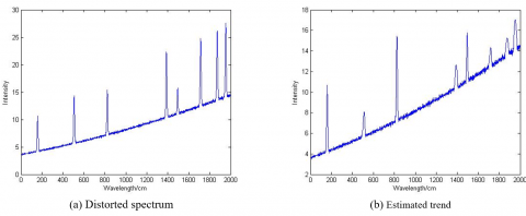
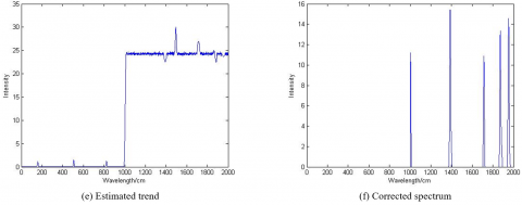
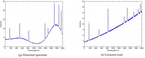
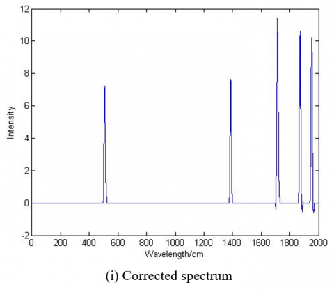
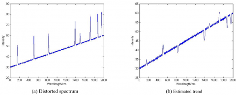
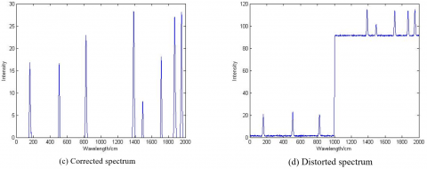
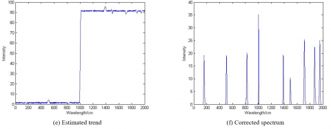
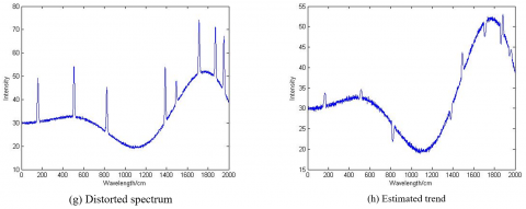
Consider a hypothetical scenario involving a distorted spectrum characterized by Gaussian noise and a linear trend, as depicted in Figure 6(a). Here, wavelet denoising is employed for noise removal. Subsequently, the trend is estimated using our proposed method of variance estimation and cubic spline interpolation, as illustrated in Figure 6(b). The subtraction of this estimated trend yields the corrected spectrum, shown in Figure 6(c).
Similarly, the results for a spectrum with a sigmoidal trend are presented in Figures 6(d)-(f). In this case, an erroneous peak is observed at the step change of the sigmoidal function. Lastly, the results for a spectrum with a sinusoidal trend are displayed in Figures 6(g)-(i), where the corrected spectrum appears to be more refined and pure.

(a) Distorted spectrum

(b) Estimated trend

(c) Corrected spectrum

(d) Distorted spectrum

(e) Estimated trend

(f) Corrected spectrum

(g) Distorted spectrum

(h) Estimated trend

(i) Corrected spectrum
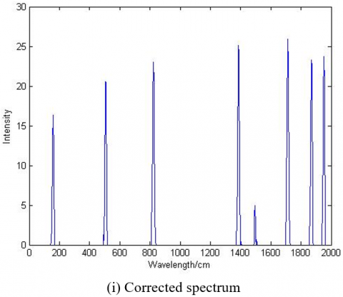
Figure 6. Wavelet denoising before trend removal results with noise variance = 0.1
Note: (a), (b), (c) are for linear trend; (d), (e), (f) are for sigmoidal trend; (g), (h), (i) are for sinusoidal trend
5.1.2 Moving average filter denoising results
The results of linear trend removal, where the moving average filter was applied initially, are demonstrated in Figures 7(a)-(c). In this instance, the estimated spectrum revealed an erroneous spike. Similarly, the outcomes of sigmoidal trend removal with the moving average filter employed as the first step are shown in Figures 7(d)-(f). In this case also, an erroneous peak is evident in the spectrum, coinciding with the step change in the sigmoidal function. Additionally, the results of sinusoidal trend removal, with the moving average filter as the primary intervention, are shown in Figures 7(g)-(i). In this scenario, one of the erroneous spikes was detected in the estimated trend, and it can be attributed to the residual noise within the spectrum, potentially leading to inaccuracies in local variance estimation. The overall performance in this case was observed to be lower than that of the wavelet denoising case.

(a) Distorted spectrum

(b) Estimated trend

(c) Corrected spectrum

(d) Distorted spectrum

(e) Estimated trend

(f) Corrected spectrum

(g) Distorted spectrum

(h) Estimated trend

(i) Corrected spectrum
Figure 7. Moving average filter denoising before trend removal results with noise variance = 0.1 (a), (b), (c) are for linear trend; (d), (e), (f) are for sigmoidal trend; (g), (h), (i) are for sinusoidal trend
5.1.3 Median filter denoising results
The results obtained with median filtering for noise reduction, followed by linear trend removal, are presented in Figures 8(a)-(c). These results indicate that the linear trend was effectively removed. In contrast, the outcomes of the sigmoidal trend removal with the median filter applied as the initial step are shown in Figures 8(d)-(f). Here, an erroneous peak is still observable in the spectrum, specifically at the point of the sigmoidal function step change. Furthermore, the results of sinusoidal trend removal with the median filter as the primary step are illustrated in Figures 8(g)-(i). In this case, there appears to be an increase in the amplitude of the wave in the estimated curve. Despite this observation, it is important to note that the overall performance in spike detection is still low.

(a) Distorted spectrum

(b) Estimated trend

(c) Corrected spectrum

(d) Distorted spectrum

(e) Estimated trend

(f) Corrected spectrum

(g) Distorted spectrum

(h) Estimated trend

(i) Corrected spectrum
Figure 8. Median filter denoising before trend removal results with noise variance = 0.1 (a), (b), (c) are for linear trend; (d), (e), (f) are for sigmoidal trend; (g), (h), (i) are for sinusoidal trend
5.1.4 Thresholding results
The results achieved through the application of the thresholding method for noise reduction after trend removal are displayed in Figures 9(a)-(c). Similarly, the outcomes with sigmoidal trend removal are shown in Figures 9(d)-(f). Moreover, the results with sinusoidal trend removal are illustrated in Figures 9(g)-(i). Upon analysis, it is evident that this approach yields the lowest performance in terms of spectrum detection. Notably, there are two spikes that are lost in the corrected spectrum. This observation underscores the inadequacy of the thresholding method in fully removing the sinusoidal trend, highlighting its limitations in certain trend removal applications.

(a) Distorted spectrum

(b) Estimated trend

(c) Corrected spectrum

(d) Distorted spectrum

(e) Estimated trend

(f) Corrected spectrum

(g) Distorted spectrum

(h) Estimated trend

(i) Corrected spectrum
Figure 9. Thresholding method before trend removal results with noise variance = 0.1 (a), (b), (c) are for linear trend; (d), (e), (f) are for sigmoidal trend; (g), (h), (i) are for sinusoidal trend
5.1.5 FFT filtering results
In this study, the FFT filtering method was applied for noise reduction after trend removal. The results for linear trend removal are illustrated in Figures 10(a)-(c). Additionally, the results for sigmoidal trend removal are presented in Figures 10(d)-(f), and those for sinusoidal trend removal are shown in Figures 10(g)-(i). However, these results elucidate that removing linear and sinusoidal trends tends to be more straightforward compared to removing sigmoidal trends. The sigmoidal trend step-change characteristic contributes to a higher MSE value. The most favorable outcomes were observed in the case of sinusoidal trend removal, as indicated by the lowest MSE values.

(a) Distorted spectrum

(b) Estimated trend

(c) Corrected spectrum

(d) Distorted spectrum

(e) Estimated trend

(f) Corrected spectrum

(g) Distorted spectrum

(h) Estimated trend
(i) Corrected spectrum
Figure 10. FFT denoising before trend removal results with noise variance = 0.1 (a), (b), (c) are for linear trend; (d), (e), (f) are for sigmoidal trend; (g), (h), (i) are for sinusoidal trend
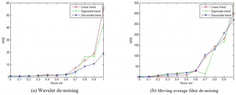
As shown in Figure 11, from the MSE perspective, the wavelet denoising technique did not exceed 2 in MSE, whereas the MSE reached higher levels of 35, 40, and even 400 to 800 for the moving average filtering, median filtering, thresholding, and FFT filtering, respectively. Upon analysis, a noticeable degradation in spike detection performance was observed. Specifically, more than three spikes were lost in the corrected spectrum across the three studied types of trend. This highlights a particular deficiency in the removal of sinusoidal trends with the FFT filtering.

(a) Wavelet de-noising

(b) Moving average filter de-noising

(c) Median filter de-noising

(d) Thresholding method de-noising

(e) FFT filter de-noising
Figure 11. MSE versus noise variance results for denoising techniques before trend removal
5.2 Denoising after trend removal
This subsection is dedicated to exploring the application of denoising subsequent to trend removal. This analysis is conducted using the same methodologies previously discussed.
5.2.1 Wavelet denoising
The results of applying wavelet denoising subsequent to linear trend removal are presented in Figures 12(a)-(c). These results clearly reveal that denoising after trend removal is not an effective approach in this context. Similarly, the outcomes of wavelet denoising following sigmoidal trend removal are shown in Figures 12(d)-(f). In this case, it is evident that denoising after trend removal results in lower performance compared to the approach in which noise is removed first. Lastly, the results of wavelet denoising after sinusoidal trend removal are illustrated in Figures 12(g)-(i). These findings indicate that for the sinusoidal trend case as well, the performance is suboptimal, especially when compared to the scenarios in which the trend removal was relatively simpler.

(a) Distorted spectrum

(b) Estimated trend

(c) Corrected spectrum

(d) Distorted spectrum

(e) Estimated trend

(f) Corrected spectrum

(g) Distorted spectrum

(h) Estimated trend

(i) Corrected spectrum
Figure 12. Wavelet denoising after trend removal results with noise of variance 0.1 (a), (b), (c) are for linear trend; (d), (e), (f) are for sigmoidal trend; (g), (h), (i) are for sinusoidal trend
5.2.2 Moving average filter
The outcomes of applying the moving average filter after linear trend removal are shown in Figures 13(a)-(c). Similarly, the results of using the moving average filter subsequent to sigmoidal trend removal are presented in Figures 13(d)-(f). Lastly, the results of employing the moving average filter following sinusoidal trend removal are illustrated in Figures 13(g)-(i). In these scenarios, while the corrected spectrum successfully captures all the appropriate spikes, it is noteworthy that the amplitude of these spikes is influenced by the presence of residual noise to some extent.

(a) Distorted spectrum

(b) Estimated trend

(c) Corrected spectrum

(d) Distorted spectrum

(e) Estimated trend

(f) Corrected spectrum

(g) Distorted spectrum

(h) Estimated trend

(i) Corrected spectrum
Figure 13. Moving average filter denoising after trend removal with noise of variance 0.1 (a), (b), (c) are for linear trend; (d), (e), (f) are for sigmoidal trend; (g), (h), (i) are for sinusoidal trend
5.2.3 Median filter
The outcomes of implementing median filtering subsequent to linear trend removal are illustrated in Figures 14(a)-(c). Furthermore, the results of median filtering following sigmoidal trend removal are shown in Figures 14(d)-(f). Additionally, the results of median filtering after sinusoidal trend removal are presented in Figures 14(g)-(i). These results collectively demonstrate that despite the application of median filtering, some noise persists in the corrected spectrum, leading to a noticeable degradation in performance.

(a) Distorted spectrum

(b) Estimated trend

(c) Corrected spectrum

(d) Distorted spectrum

(e) Estimated trend

(f) Corrected spectrum

(g) Distorted spectrum

(h) Estimated trend

(i) Corrected spectrum
Figure 14. Median filter denoising after trend removal with noise of variance 0.1 (a), (b), (c) are for linear trend; (d), (e), (f) are for sigmoidal trend; (g), (h), (i) are for sinusoidal trend
5.2.4 Thresholding
Figures 15(a)-(c) display the results obtained when thresholding is applied following linear trend removal. The outcomes of applying thresholding after sigmoidal trend removal are given in Figures 15(d)-(f). Additionally, Figures 15(g)-(i) present the results of thresholding subsequent to sinusoidal trend removal. These results reveal a notable distortion in the corrected spectrum. It is observed that not only does some noise remain, but also the trend has not been completely removed, indicating a low efficacy of the thresholding process in these scenarios.
Figure 15. Thresholding after trend removal with noise of variance 0.1 (a), (b), (c) are for linear trend; (d), (e), (f) are for sigmoidal trend; (g), (h), (i) are for sinusoidal trend
5.2.5 FFT filter
Figures 16(a)-(c) illustrate the results achieved using the FFT filter after linear trend removal. The outcomes of the FFT filter applied subsequent to sigmoidal trend removal are shown in Figures 16(d)-(f). Additionally, Figures 16(g)-(i) present the results of applying the FFT filter following sinusoidal trend removal. These results highlight a significant limitation: the FFT filter fails to effectively reconstruct spikes from the noisy spectrum in the cases of both linear and sinusoidal trends, indicating a shortfall in its denoising capability in these specific scenarios.
Figure 16. FFT filter denoising after trend removal with noise of variance 0.1 (a), (b), (c) are for linear trend; (d), (e), (f) are for sigmoidal trend; (g), (h), (i) are for sinusoidal trend
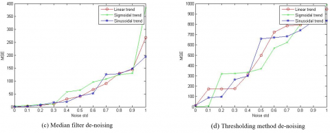
Figure 17. MSE versus noise variance results for denoising techniques after trend removal
Figure 17 presents a comparative analysis from an MSE perspective, detailing the outcomes obtained for various trends using different denoising techniques. Interestingly, the results across all techniques are closely aligned. However, these figures indicate that the removal of linear and sinusoidal trends is generally more straightforward compared to the removal of sigmoidal trends. This complexity in removing sigmoidal trends is attributed to the step change inherent in their shape, resulting in large MSE values. Notably, the results for sinusoidal trend removal stand out as the most effective, as evidenced by the lowest MSE values achieved. The MSE for wavelet denoising remains below 60, whereas it escalates to 400, 350, and 1000 for the moving average filter, median filter, and thresholding, respectively. In this context, the MSE is approximately tenfold higher than those in scenarios in which noise removal was prioritized.
The analysis of these results shows that wavelet denoising is the most efficient among the tested denoising techniques, maintaining the lowest MSE values even under high noise deviations. It is apparent across all studied denoising techniques that sinusoidal trend removal is less challenging compared to other trend types (linear, sigmoidal), primarily because spline interpolation adeptly estimates sinusoidal trends. Conversely, the sigmoidal trend removal shows the highest error, largely due to the step change in the signal. Moreover, it is observed that applying denoising to a noisy spectrum before trend removal yields better results than applying trend removal first. These findings are systematically summarized in Tables 1-3, wherein the noise variance is consistently set at 0.1.
Table 1. MSE for different denoising techniques before trend removal
|
Denoising Technique |
MSE-Linear Trend |
MSE-Sigmoidal Trend |
MSE-Sinusoidal Trend |
|
Wavelet denoising |
0.09 |
0.58 |
0.08 |
|
Moving average filter |
0.31 |
0.83 |
0.36 |
|
Median filter |
0.83 |
5.06 |
0.80 |
|
Thresholding |
0.87 |
5.15 |
0.86 |
|
FFT Filter |
9.49 |
17.7 |
9.01 |
Table 1 displays the MSE values for various denoising techniques implemented before trend removal. With the wavelet denoising technique, the MSE values for linear, sigmoidal, and sinusoidal trend removal are 0.09, 0.58, and 0.08, respectively. The moving average filter shows MSE values of 0.31, 0.83, and 0.36 for linear, sigmoidal, and sinusoidal trend removal, respectively. With the median filter technique, the MSE values are 0.83, 5.06, and 0.80 for linear, sigmoidal, and sinusoidal trend removal, respectively. The thresholding technique reports MSE values of 0.87, 5.15, and 0.86 for linear, sigmoidal, and sinusoidal trend removal, respectively. For the FFT filter technique, the MSE values for linear, sigmoidal, and sinusoidal trend removal are significantly higher, with values of 9.49, 17.7, and 9.01, respectively. The results across these techniques exhibit close proximities.
Table 2. MSE for different denoising techniques after trend removal
|
Denoising Technique |
MSE-Linear Trend |
MSE-Sigmoidal Trend |
MSE-Sinusoidal Trend |
|
Wavelet denoising |
0.65 |
0.85 |
0.65 |
|
Moving average filter |
2.5 |
4.9 |
1.2 |
|
Median filter |
1.16 |
1.7 |
1.10 |
|
Thresholding |
173 |
279 |
88.33 |
|
FFT Filter |
249 |
402 |
212 |
Table 3. MSE for sinusoidal trend removal in the two cases
|
Denoising Technique |
Denoising before Trend Removal |
Denoising after Trend Removal |
|
Wavelet denoising |
0.08 |
0.65 |
|
Moving average filter |
0.31 |
1.2 |
|
Median filter |
0.80 |
1.10 |
|
Thresholding |
0.86 |
88.33 |
|
FFT Filter |
9.01 |
212 |
Table 2 presents the MSE values for different denoising techniques applied after trend removal. The wavelet denoising technique yields MSE values of 0.65, 0.85, and 0.65 for linear, sigmoidal, and sinusoidal trend removal, respectively. The moving average filter technique shows MSE values of 2.5, 4.9, and 1.2 for linear, sigmoidal, and sinusoidal trend removal, respectively.
Table 4. Comparison between Kandjani’s algorithm and the proposed algorithm
|
Features |
Kandjani′s Algorithm [9] |
Proposed Algorithm |
|
Basic concept |
Coupling continuous wavelet transform with signal removal method. |
Local variance estimation and cubic spline interpolation. |
|
Processing time |
Long time (120 sec). (140-220 sec) with noise having variance = 0.1. |
Less time (12 sec) without noise. (50-70 sec) with noise having a variance = 0.1. |
|
RMS Error |
(0.1 to 0.2) without noise. (1 to 5) with noise having variance = 0.1. |
(0.001 to 0.0015) without noise. (0.08 to 1) with noise having a variance = 0.1 (wavelet denoising technique). |
|
Advantages |
Smoothing-free algorithm. |
Smoothing-free algorithm. Complexity free. Less error and processing time. |
|
Disadvantages |
Many complicated calculations. Long processing time. The peaks overlap with each other when the distance between peaks becomes less than their width. RMSE increases with the increase in the number of peaks. |
If the peak amplitude is small, variance is small, and peaks get lost. Interpolation is not suitable for very wide peaks removed. |
A detailed comparison between the proposed algorithm and Kandjani’s algorithm [9] is presented in Table 4. Kandjani’s algorithm, which combines continuous wavelet transform with signal removal method for trend removal, requires a large processing time of approximately 120 seconds without additive noise and 140-220 seconds with additive noise. In contrast, the proposed algorithm demonstrates more efficiency, requiring only about 12 seconds without additive noise and 50-70 seconds with additive noise. The MSE of Kandjani’s algorithm ranges from 0.1 to 0.2 without noise and 1 to 5 with noise having a variance of 0.1, whereas the proposed algorithm exhibits a lower MSE of approximately 0.001 to 0.0015 without noise and 0.08 to 1 with noise having a variance of 0.1 (specifically for the wavelet denoising technique with sinusoidal trend).
Both algorithms are free of smoothing complexities, but the proposed algorithm stands out for its reduced error and less processing time. Kandjani’s algorithm, despite its effectiveness, is limited by its large processing time and the potential for peak overlap, when the distance between peaks is less than their width. In contrast, the proposed algorithm may encounter challenges in detecting peaks with small amplitude, small variance, or when the interpolation is not ideally suited for wide peaks that have been removed.
This paper presented a study of simultaneous denoising and trend removal, specifically focusing on the Raman spectrum. The choice of the Raman spectrum is due to its characteristics of low Signal-to-Noise Ratio (SNR) and trends with large magnitudes. A key finding from this study is that the wavelet denoising emerges as the most effective denoising technique across all the cases examined. Additionally, it has been observed that applying denoising to a signal prior to trend removal yields better results than conducting the trend removal, initially. Specifically, in the sinusoidal case, trend removal was found to be more straightforward compared to the sigmoidal and linear trend cases. The insights garnered from this study are particularly relevant and applicable in the fields of physics, chemistry, and biology. Given its broad applicability and effectiveness, this research is of considerable value, especially in developing regions such as countries in Africa, where such advanced analytical techniques can greatly enhance scientific and technological capabilities.
•Limitations of this study
Scope of spectrum types: While the study extensively explores the Raman spectrum, the application of the proposed denoising and trend removal techniques may have varying degrees of effectiveness on other types of spectra. Future studies could expand to include a wider range of spectrum types.
Algorithm complexity: The proposed algorithm, especially with cubic spline interpolation, may involve computational complexities that could affect its efficiency in real-time applications. Furthermore, optimization of the algorithm could be explored to enhance its applicability.
Noise variability: The study primarily focuses on scenarios with low SNR and trends with large magnitudes. The performance of the proposed techniques in situations with different noise characteristics, such as higher SNR or different noise types, needs to be thoroughly examined.
Hardware limitations: The effectiveness of the proposed techniques in a real-world settings may be influenced by hardware capabilities.
•Future work
Broadening the spectrum range: Future research could investigate the application of the proposed algorithms to different types of spectroscopic data, such as infrared or ultraviolet spectra, to assess their versatility and adaptability.
Algorithm optimization for real-time analysis: Developing more computationally efficient versions of the proposed algorithms would be valuable, especially for real-time spectral analysis applications.
Exploring automated trend identification: Automating the process of trend identification could enhance the usability of the proposed techniques, making them more accessible to users without extensive technical expertise.
Adaptation to different noise types and levels: Further research could focus on adapting the proposed techniques to handle a wider range of noise types and levels, ensuring broader applicability.
Hardware-software integration: Investigating the integration of the proposed techniques with different types of spectroscopic hardware, particularly in resource-limited settings, would be crucial to enhance their practicality and accessibility.
Cross-disciplinary applications: Exploring the application of these techniques in various scientific fields, such as environmental monitoring or medical diagnostics, could open new directions for research and development.
The authors would like to acknowledge the support from Princess Nourah bint Abdulrahman University Researchers Supporting Project number (PNURSP2025R138), Princess Nourah bint Abdulrahman University, Riyadh, Saudi Arabia.
[1] Khan, M., Do Nascimento, G.M., El-Azazy, M. (2020). Modern Spectroscopic Techniques and Applications. BoD–Books on Demand. https://www.academia.edu/107382823/Modern_Spectroscopic_Techniques_and_Applications_Working_Title.
[2] Gierlinger, N., Schwanninger, M. (2007). The potential of Raman microscopy and Raman imaging in plant research. Journal of Spectroscopy, 21(2): 69-89. https://doi.org/10.1155/2007/498206
[3] Eichmann, S.C., Trost, J., Seeger, T., Zigan, L., Leipertz, A. (2011). Application of linear Raman spectroscopy for the determination of acetone decomposition. Optics Express, 19(12): 11052-11058. https://doi.org/10.1364/OE.19.011052
[4] Luo, Y., Hargraves, R.H., Belle, A., Bai, O., Qi, X.G., Ward, K.R., Pfaffenberger, M.P., Najarian, K. (2013). A hierarchical method for removal of baseline drift from biomedical signals: Application in ECG analysis. The Scientific World Journal, 2013(1): 896056. https://doi.org/10.1155/2013/896056
[5] Mazet, V., Carteret, C., Brie, D., Idier, J., Humbert, B. (2005). Background removal from spectra by designing and minimising a non-quadratic cost function. Chemometrics and Intelligent Laboratory Systems, 76(2): 121-133. https://doi.org/10.1016/j.chemolab.2004.10.003
[6] Zhang, Z.M., Chen, S., Liang, Y.Z. (2010). Baseline correction using adaptive iteratively reweighted penalized least squares. Analyst, 135(5): 1138-1146. https://doi.org/10.1039/b922045c
[7] Schulze, G., Jirasek, A., Yu, M.M., Lim, A., Turner, R.F., Blades, M.W. (2005). Investigation of selected baseline removal techniques as candidates for automated implementation. Applied Spectroscopy, 59(5): 545-574. https://doi.org/10.1366/0003702053945985
[8] Liu, B.F., Sera, Y., Matsubara, N., Otsuka, K., Terabe, S. (2003). Signal denoising and baseline correction by discrete wavelet transform for microchip capillary electrophoresis. Electrophoresis, 24(18): 3260-3265. https://doi.org/10.1002/elps.200305548
[9] Kandjani, A.E., Griffin, M.J., Ramanathan, R., Ippolito, S.J., Bhargava, S.K., Bansal, V. (2013). A new paradigm for signal processing of Raman spectra using a smoothing free algorithm: Coupling continuous wavelet transform with signal removal method. Journal of Raman Spectroscopy, 44(4): 608-621. https://doi.org/10.1002/jrs.4232
[10] Schulze, H.G., Foist, R.B., Okuda, K., Ivanov, A., Turner, R.F. (2011). A model-free, fully automated baseline-removal method for Raman spectra. Applied Spectroscopy, 65(1): 75-84. https://doi.org/10.1366/10-06010
[11] Jebur, R.S., Der, C.S., Hammood, D.A., Weng, L.Y. (2023). Image denoising techniques: An overview. AIP Conference Proceedings, 2804(1): 020002. https://doi.org/10.1063/5.0154497
[12] Baek, C., Düker, M.C., Pipiras, V. (2023). Local Whittle estimation of high-dimensional long-run variance and precision matrices. The Annals of Statistics, 51(6): 2386-2414. https://doi.org/10.1214/23‑AOS2330
[13] Zhang, Y., Wang, L., Zhao, J., Yao, W. (2023). Python-based cubic B-spline interpolation algorithm for pump characteristic curves. In Third International Conference on Mechanical Design and Simulation (MDS 2023), Xi'an, China, pp. 395-400. https://doi.org/10.1117/12.2681838
[14] Mortada, B., EI-Babaie, E.S.M., EI-Kordy, M.F., Zahran, O., EI-Samie, F.E.A. (2015). Trend removal from Raman spectra With local variance estimation and cubic spline interpolation. Circuits and Systems: An International Journal, 2(1): 1-12.
[15] Ahmad, K., Khan, J., Iqbal, M.S.U.D. (2019). A comparative study of different denoising techniques in digital image processing. In 2019 8th International Conference on Modeling Simulation and Applied Optimization (ICMSAO), Manama, Bahrain, pp. 1-6. https://doi.org/10.1109/ICMSAO.2019.8880389
[16] Gupta, D., Ahmad, M. (2018). Brain MR image denoising based on wavelet transform. International Journal of Advanced Technology and Engineering Exploration, 5(38): 11-16. https://doi.org/10.19101/IJATEE.2017.437007
[17] Fedak, V., Nakonechny, A. (2015). Adaptive wavelet thresholding for image denoising using sure minimization and clustering of wavelet coefficients. Czasopismo Techniczne, pp. 197-210. https://doi.org/10.4467/2353737XCT.15.096.3928
[18] Sharma, P., Kaur, A. (2013). Comparison of different techniques of digital image denoising. International Journal of Engineering Research Technology, 2(4): 417-420. https://doi.org/10.17577/IJERTV2IS4370
[19] Dangeti, S.V. (2003). Denoising techniques – A comparison. M.S. Thesis, Louisiana State University and Agricultural & Mechanical College. https://repository.lsu.edu/gradschool_theses/3789/.
[20] Kong, Z., Deng, F., Zhuang, H., Yu, J., He, L., Yang, X. (2023). A comparison of image denoising methods. arXiv preprint arXiv:2304.08990. https://doi.org/10.48550/arXiv.2304.08990
[21] Otsu, N. (1975). A threshold selection method from gray-level histograms. Automatica, 11(285-296): 23-27. https://doi.org/10.1109/TSMC.1979.4310076
[22] Singh, N., Oorkavalan, U. (2018). Triple Threshold Statistical Detection filter for removing high density random-valued impulse noise in images. EURASIP Journal on Image and Video Processing, 2018(1): 22. https://doi.org/10.1186/s13640-018-0263-0
[23] Jones, K.J. (2006). Flexible-length fast Fourier transform for mapping onto single-instruction multiple-data computing architecture. IEE Proceedings-Vision, Image and Signal Processing, 153(4): 395-404. https://doi.org/10.1049/ip‑vis:20050039